A Constraint programming-based genetic algorithm for capacity output optimization

JIEM, 2014 – 7(5): 1222-1249 – Online ISSN: 2013-0953 – Print ISSN: 2013-8423 http://dx.doi.org/10.3926/jiem.1070

A Constraint Programming-based Genetic Algorithm (CPGA) for

Capacity Output Optimization

Kate Ean Nee Goh

_{, Jeng Feng Chin}

_{, Wei Ping Loh}

_{, Melissa Chea-Ling Tan}

1

_{School of Mechanical Engineering, Universiti Sains Malaysia (Malaysia)}

2

_{Ines-Nathan Creative Research Center (Malaysia)}

[email protected], [email protected], [email protected], [email protected]

Received: January 2014

Accepted: October 2014

Abstract:

Purpose:

The manuscript presents an investigation into a constraint programming-based

genetic algorithm for capacity output optimization in a back-end semiconductor manufacturing

company.

Design/methodology/approach:

In the first stage, constraint programming defining the

relationships between variables was formulated into the objective function. A genetic algorithm

model was created in the second stage to optimize capacity output. Three demand scenarios

were applied to test the robustness of the proposed algorithm.

Findings:

CPGA improved both the machine utilization and capacity output once the

minimum requirements of a demand scenario were fulfilled. Capacity outputs of the three

scenarios were improved by 157%, 7%, and 69%, respectively.

Practical implications:

Capacity planning in a semiconductor manufacturing facility need to

consider multiple mutually influenced constraints in resource availability, process flow and

product demand. The findings prove that CPGA is a practical and an efficient alternative to

optimize the capacity output and to allow the company to review its capacity with quick

feedback.

Originality/value:

The work integrates two contemporary computational methods for a real

industry application conventionally reliant on human judgement.

Keywords:

constraint programming, genetic algorithm, semiconductor capacity management,

production planning

1. Introduction

Capacity planning aims to minimize the discrepancy between organization capacity and the product demands to optimize revenue. Capacity planning in semiconductor industry is extremely challenging due to its product mix, limited capacity of resources and uneven demands. Consequentially, a semiconductor manufacturing company needs to balance heterogeneous set of products with different required time or resources in production (Naughton, 2005).

Resources typically include machines, labor, money, time, and raw materials. The resource cost is commonly a considerable production cost in semiconductor industry. Of these resources, machines are the most critical due to their expensive costs and long acquisition periods. A way for the capacity of expensive resources to be highly utilized is through machine sharing. Machines share their capability to cope with product mixes, which allows changes of one product to another in the same machine (Qiu, Joshi & Mcdonell, 2004). By improving machine utilization, capacity output is maximized, which in return results in revenue gains to the company. One example is semiconductor assembly and testing (back-end (BE) production) industry, in which the equipment cost ranges from twenty thousands to almost a million US dollars. For an assembly and testing facility with 80 sets of tools, the total amount of capital investment requires approximately 16 million US dollars. Saving on capacity could result in gain of a few hundred thousand per year. A 5% savings on capacity result in 160 thousands dollars per year with five-year depreciation.

(Yusof & Deris, 2010). Integrating several factors that affect capacity allocation, such as operation routings, multiplicity types of resources and products, capability of resources, and flexibility to cater unexpected what-if scenarios (e.g. shift in demand) and constraints in machine sharing, have been somewhat neglected, simplified and dealt separately (Wang, Wang & Chen, 2008b). Capacity allocation is further complicated as BE operations are closer to customer and have shorter cycle time than front-end operations (Guo, Chiang & Pai, 2007). This setting results in a smaller time buffer to react to changes. With shorter decision time for capacity allocation, top managements need quick and accurate capacity allocation in the presence of demand change, essentially to ensure sufficient capacity and on-time delivery of finished goods for customer satisfaction. Another concern is the capability of the machines to maximize output following product mix changes.

Motivated by the foregoing factors, this research develops an efficient approach to maximize capacity output and machine utilization using constraint programming-based genetic algorithm (CPGA). The approach provides a near optimal solution in spite of the changes in product mix order. A real case study was taken from BE production.

The rest of the paper is prepared as follows. Section 2 reviews the related work. Section 3 describes the case study company. Section 4 presents the research methodology. Section 5 describes the problem formulation. Section 6 describes an implementation of the proposed method. Section 7 discusses the results of the proposed solution. Section 8 concludes the study.

2. Literature review

scenario-based stochastic programming model to describe the uncertain capacity scenario-based on overall equipment efficiency. Chen and Lu (2012) discussed how the stochastic mixed-integer programming model could be used to determine the robust capacity allocation and expansion policy. Swaminathan (2000) provided heuristics to find efficient tool procurement plans and test their quality using Lagrangian relaxation. Phruksaphanrat, Ohsato and Yenradee (2011) proposed aggregate Production Planning model to deal with fuzzy demand and variable system capacity. The new model achieves higher flexibility in estimation and better production plan. Many studies have been conducted to find the tool procurement plan by optimizing the tool capacity allocation. The mathematical-based modeling and exact solution methods are accurate. However, they are usually time consuming due to the complexity of the problems (Wang et al., 2008a). The optimality of the solution depends on the problem domain, given that the variables to be considered are limited.

In comparison, computation models allow rapid generation of fairly good solutions for considerably more complex capacity planning problems (Zhang, 2007; Bilgin & Azizoğlu, 2009; Hsu & Li, 2009). The models derived from artificial intelligence and taking advantage of iterative metaheuristic application of controlled randomization on cumulative results. Metaheuristic algorithms imitate the characteristic of natural-inspired (based on some principles from physics, biology or ethology) (Boussaïd, Lepagnot & Siarry, 2013). Genetic algorithm (GA) is the most popular metaheuristic model to resolve resource-planning problems (Wang et al., 2008a). GA is based on the concept that a population of candidate solutions should be created and then subjected to an evolutionary process to generate the offspring candidate according to the selection criteria (Schneider, 2002).

Zhang (2007) developed a heuristic algorithm, which involves the combination of the GAs and primal-dual algorithm of nonlinear programming, to solve capacity planning under uncertain demand and production consumption. Wang et al. (2008b) proposed a stochastic programming-based GA to determine a profitable capacity planning and task allocation plan. Wang et al. (2008a) proposed an immune-genetic algorithm to improve the performance of GA in complex constrained optimization problems. Abazari, Solimanpur and Sattari (2012) applied GA to find the effective solution from the formulated formula to solve the machine loading problem in flexible manufacturing systems. Li, Jiang and He (2014) developed a genetic-algorithm based method to solve a complex equipment-workforce-service planning problem.

and a controllable process of innovation (Bajpai & Kumar, 2010). Since the problem is highly complex, a GA is sought to solve the problem efficiently.

Other notable computer models include tabu search, simulated annealing, and ant colony optimization. Bilgin and Azizoğlu (2009) used tabu search algorithm to optimize the capacity allocation in the semiconductor industry. Hsu & Li (2009) developed a heuristic solution approach based on simulated annealing to determine the optimal adjusting decisions regarding production reallocation under fluctuating demand. Other evolutionary methods used the ant colony optimization and particle swarm optimization.

Computer models, despite relative simplicity in programming, do not guarantee optimal solution. They are approximation techniques in which solution qualities are influenced by the representation, parameters, and problem domain. The development of objective function needs to encompass all the factors of interest, particularly the real-life problems.

Constraint programming (CP) is often integrated into computer models, such as GA, to solve the foregoing problems. GA is a search method to identify the near optimal solution for the objective function. CP is a methodology for declarative description and solution of difficult combinatorial problems, particularly in the areas of planning and scheduling (Barták, 1999). The basic idea in CP is that the user states the constraints (requirements) in the problem area (Rossi, Van Beek, Walsh, 2006). Constraints map out how variables in the program must relate to each other. Each variable take a value in a given domain. The constraint thus restricts the possible values that variables can take. The important feature of constraints is their declarative manner. They define what relationship must hold within the variables without specifying a computational procedure to enforce the relationship. A feasible solution needs to satisfy all the constraints and minimize or maximize the objective function, respectively (Barták, 1999). The quality of solution is usually measured by an application-dependent function referred to as objective function. CP ensures the compliance of the genes with the predefined constraint network (Chiu & Hsu, 2005), thereby accelerating the evolution process in GA by implicitly guiding the chromosome generation. Van Beek and Chen (1999) presented evidence that CP approach can work well in planning and has the advantage in terms of time and space efficiency. Kovács, Váncza, Kádár, Monostori and Pfeiffer (2003) implemented the integration of CP and simulation to evaluate the robustness of scheduling problems by considering various uncertainties.

3. Case study

Company A, a multinational BE semiconductor manufacturing company located in Penang, with approximately 4,600 employees, was used as the case study. Company A supplies customers from approximately 150 countries worldwide. In 2012, the company achieved a turnover of 5 billion Euro. Company A manufactures products, such as light emitting diodes for automotive, consumer, and industrial applications, infrared products, laser diodes, and optical sensors.

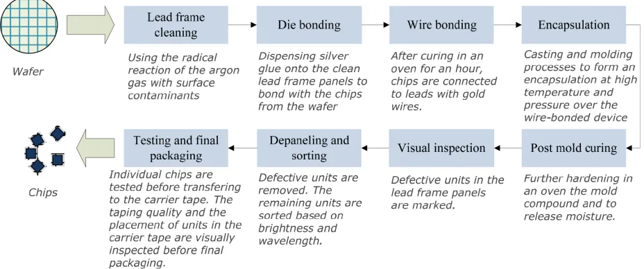
Company A uses lead frame in manufacturing chip packages. The lead frame is in panel form, which is arranged in a matrix that is extended in multiple rows and columns. The total number of units produced from one lead frame panel is different from others based on the size of the chip packages. The lead frame moves through the assembly facilities in a lot (collection of lead frame panels). A number of processing steps are performed by the single lead frame panel, while other steps are performed on the entire lot, with several lots processed at the same time. The whole processing steps are depicted in Figure 1.

Figure 1. BE processing steps

This study investigates an approach that can maximize both the output and utilization of largely shared machines. The specific manufacturing period ranges from one month to six months. Prediction of demand over a period requires a short-term planning that relies on customer forecasts and committed order and work in progress (WIP) levels. Frequent revision on customer orders is normal before confirmation. The manufacturing lead time was approximately two weeks. The manufacturing production quantities and product mixes were adjusted according to latest company forecast and strategic needs.

An actual capacity planning problem extracted from Company A consists of six product types, eight operation routings, and nine resources types. One year data was collected from various sources, including meetings and teleconferences, collected progress reports, bug reports, and other documentations from Company A. To protect proprietary information without affecting the validity of the case study, the product and resource names have been disguised. The products were clustered under a product family as machines were shared among these products. The sharing capability of machine is attributed to machine’s permissible configurability for different product types. The machine technology in each operation can run for several product types (consisted in product family). However, it may have a different processing time.

4. Research methodology

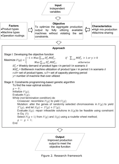
The study involves two main stages: developing objective function and capacity output optimization. Figure 2 depicts the research framework. The first stage develops the objective function, which aims to provide valuable insight into how capacity varies with suspected changes in resource availability, resource efficiency, process improvement, process flow, or product demand. In this stage, the product–resource–operation relationship is described and CP is modeled. The inherent characteristics of the case problem include high mix production and machine sharing. Microsoft Excel Spreadsheets are used to contain the capacity data and to compute objective function.

Figure 2. Research framework

5. Constraints formulation

5.1. Stage I: Developing the objective function

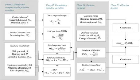
First, a collection of variables need to be determined. Part of the modeling task is to identify the decision variables from the primitive variables. The variables included in modeling the CP are stated as follows:

Primitive Variables

Demand quantity of product type r in period t in scenario δ

MOi,t Available number of machine type i in period t

TEi,r Percentage of total effective equipment performance (TEEP) of machine type i in

product type r

S Number of shifts per week

H Number of hours per shift

Yr Process yield for product type r

Ui,r Unit per hour of product type r in machine type i

PTi,r Processing time of product type r in machine type i

Gt,r Gross required output needed for product type r in period t

RUi,t,r Total utilized hour of product type r in machine type i in period t

AHi,r Total available operating hour of product type r in machine type i

EAi Percentage of equipment availability for machine type i

OE Operating efficiency

RQi,r Rate of quality

Decision Variables

DMt,r Maximum demand quantity of product type r in period t

DLt,r Minimum demand quantity of product type r in period t

Type i machine utilization for product type r in period t in scenario δ

Ai,r The machine type i production ability to manufacture product type r, where i  I, which

is a set of machines types. Ai,r = a Boolean parameter Ai,r = 1 when machine type i can produce product type r; Ai,r = 0 otherwise).

The change of product demand type r in period t in scenario δ. is a Boolean

parameter ( = 1 when demand is subjected to change; = 0 otherwise).

y Number of machine that is over utilized

where

i = Set of machine type (i = 1, …, I)

r = Set of product type (r = 1, …, R)

t = Set of capacity planning period (t = 1, …, T

)

δ = Index of demand scenario (δ = 1, …)

The objective function is then formulated in this problem. The purpose is to maximize the total capacity output of the different types of products by fully utilizing the bottleneck machines in each demand scenario, as in section 5.1. The demand scenario is explained in Section 6. The machines from set I, with the highest ratio of machine utilization required to set the product type r at scenario δ, are considered the bottleneck.

(1)

Where = , " t  T, " i  I.

Subjected to the following constraints:

Limited resource

The machine utilization must be less than or equal to 100%. The machine cannot be over-utilized (Equation 2 and 3).

No machine is over-utilized,

y= 0 (3)

Quantity of promised demand from customer.

The required demand quantity must be less than or equal to the available capacity provided by the machines (Equation 4).

,"tT,"iI. ₍₄₎

Demand range

The required demand quantity must be within the set range of maximum and minimum demand quantities of product type r in period t The minimum value is based on aggregate firm or committed customer orders whereas the maximum value is the optimistic demand forecast given by the business unit. High runner products normally will be assigned with larger maximum values.

(5)

Capacity balance

The total required utilized hours must be equal or less than the available operating hours.

,"iI. (6)

, if product type r is unable to run by machine type i

1996). In this study, the formulations were modified as shown in phases demonstrated in Figure 3.

The assumptions applied in modeling the CP are as follows:

i. Current work in process (WIP) is not considered.

ii. Queue time and material handling time are either assumed to be zero or are incorporated to the processing time of the resource.

iii. All scheduled downtime are static and not subjected to stochastic variations.

iv. The machine breakdown time is obtained from the factory control system.

v. Profit of different product unit types is equal.

vi. The complexity of the problem increases exponentially with the increase of product types, machine types, and operation routings.

vii. One month equates to 4.17 weeks.

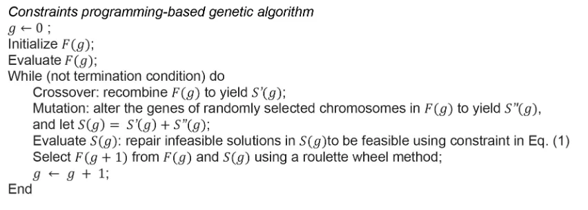
5.2. Stage II: Constraint programming-based genetic algorithm (CPGA)

CPGA was used to optimize the capacity output. CPGA described the interaction between the objective function from the CP and the genetic operators, as shown in Figure 4.

F(g) and S(g) represent the parents and offsprings of a generation (g), respectively. The input parameters are chromosome size, crossover, and mutation rate. An initial population of chromosomes of size N is generated. The chromosome is made up of a sequence of binary numbers represented by ‘0’ or ‘1’. The length of chromosome was based on the number of

product types subjected to demand change, . Each chromosome consists the number of

genes that represent the quantity of a particular product type. The size of the gene or the number of bits used to represent a variable is important for the accuracy of the solution and the time needed for the GA to converge (Haupt & Haupt, 2004). Although 4-bit string contributes faster convergence of algorithm (Yusof & Deris, 2010), the gene in this study is represented by 8-bit string, as the increased number of bits would help reducing quantization error (Haupt & Haupt, 2004).

Figure 4. Constraints programming-based genetic algorithm

A chromosome for six product types is constructed indicating 48-bits strings, as shown in Figure 5. The populations were assigned a fitness value which was evaluated using the equation. The fitness function decides if the bottleneck machines have been fully occupied for the highest capacity output of all product types.

The initial population was modified by the genetic operators, namely, selection, crossover, and mutation, to improve fitness. Following Haupt and Haupt (2004), the standard approach, roulette wheel selection, was normally used. Each chromosome received a portion of a roulette wheel according to relative fitness. Larger reflected portion corresponded to a better fitness value and higher chance of selection. The roulette wheel was spun and the corresponding chromosome was selected when the arrow rested at one of the portions. The sizes of chromosome population remained unchanged from one generation to the next. The roulette wheel was spun 10 times to establish the same population size. This setup means 10 chromosomes were passed to the next generation.

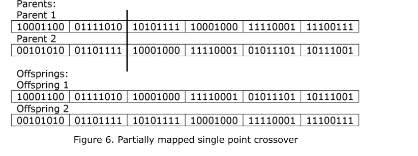
Crossover and mutation were repeated until satisfactory result was achieved. Partially mapped and cycle crossover were applied (Yusof & Deris, 2010). Partially mapped single point crossover was selected as it can perform better than cycle crossover (Chen & Smith, 1996). In the partially mapped single point crossover, a crossover point, or kinetochore, was randomly selected between the first and last bits of the parent chromosomes. For example, Parent 1 and Parent 2 could be crossed over after the second gene in each parent produces two offsprings (Figure 6). Mutation is equivalent to random search; its role is to provide a guarantee that the search algorithm is not trapped on a local optimum. For the binary GA, this observation amounted to changing a bit from a 0 to a 1, and vice versa (Haupt & Haupt, 2004). Thus, bit string mutation is used. The mutation of bit strings ensues through bit flips at random positions. An 8-bit gene was randomly selected from the corresponding gene pool. In the example shown in Figure 7, the chromosome is mutated in its 5th gene, which shows that 01000101 is mutated to 01001101 (randomly flip bit from 0 goes to 1 and 1 goes to 0). CPGA was terminated after a specified number of generations and the best chromosome found in the population was chosen.

The solution violating Equation 2, 3, and 5 was not feasible and would be implicitly removed through backtracking. In the backtracking process, these infeasible solutions were identified

and have their objective function rephrased to . Consequentially, negative

fitness values were produced and effectively made these solutions unattractive and unlikely to survive to the next generation. The process continued until F(g) was assigned a positive value.

6. Implementation

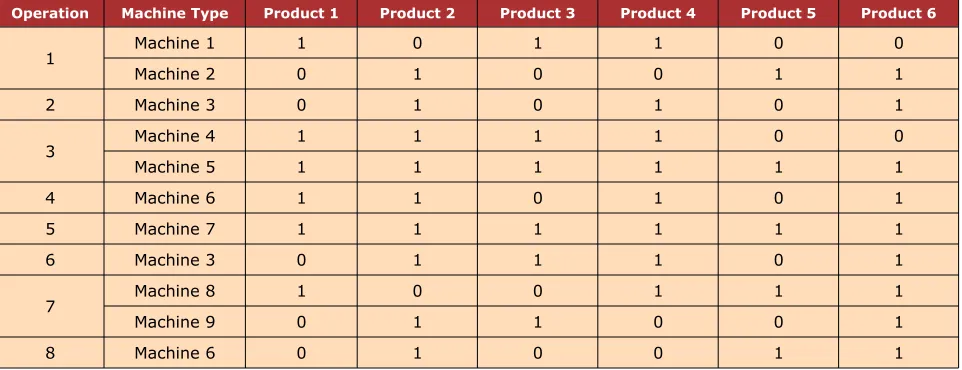
Table 1 shows products produced based on machine types and the operation routings. When

ith type of machine can produce product type r, then Ai,r= 1. Conversely, Ai,r = 0.

Table 1 illustrates the three-point relation (product–resource–operation). Similar machines can be used to run different operations. For example, Machine 3 can be operated in both Operations 2 and 6 by changing the materials used in each operation. Thus, the utilized hours of Machine 3 is the sum of hours needed from both operations. Each product has individual operation flow. For instance the operation flow for Product 1 is 1  3  4  5  7, while

Product 2 is 1  3  4  5  6  7  8. Each operation is carried out by one or more

machine types. Operation 1 involves two machine types, Machines 1 and 2, whereas Operation 2 only involves one machine type, Machine 3. The three-point relationship is important because any wrong declaration on the production machine feasibility would affect the results of the machine utilization decision function and generate invalid capacity output.

Operation Machine Type Product 1 Product 2 Product 3 Product 4 Product 5 Product 6

1 Machine 1 1 0 1 1 0 0

Machine 2 0 1 0 0 1 1

2 Machine 3 0 1 0 1 0 1

3 Machine 4 1 1 1 1 0 0

Machine 5 1 1 1 1 1 1

4 Machine 6 1 1 0 1 0 1

5 Machine 7 1 1 1 1 1 1

6 Machine 3 0 1 1 1 0 1

7 Machine 8 1 0 0 1 1 1

Machine 9 0 1 1 0 0 1

8 Machine 6 0 1 0 0 1 1

1: Feasible relationship; 0: Infeasible relationship.

The total number of hours utilized for each machine type is based on the unit per hour (UPH), which delineates the quantity of the product produced within an hour. Table 2 shows the gross UPH of product type r in machine type i for each operation. UPH varies for different products that run on the same machine type or for the same product that run on different machine types. Following the company practice, the UPH was adjusted to account for efficiency losses including the defects, scraps machine breakdowns and machine setups. Consequentially, any machine meeting the UPH would have achieved the full utilization in the calculation but not in reality. In capacity planning, the machines that produced higher UPH under same the operation and product type are given the top priority. For instance, both Machines 4 and 5 can be used to run Operation 3 for Product 1. However, Machine 4, which provides higher UPH, was given the higher priority.

Operation Machine Type Product 1 Product 2 Product 3 Product 4 Product 5 Product 6

1 Machine 1 8,400 - 10,800 10,500 -

-Machine 2 - 8,000 - - 6,400 9,600

2 Machine 3 - 9,000 - 8,500 - 12,000

3 Machine 4 9,000 9,000 8,500 8,000 -

-Machine 5 7,000 9,000 8,500 8,000 4,500 3,000

4 Machine 6 9,500 9,200 - 10,860 - 8,840

5 Machine 7 5,000 5,000 6,000 5,500 5,700 5,500

6 Machine 3 - 9,000 8,000 8,500 - 12,000

7 Machine 8 9,000 - - 9,000 9,000 9,000

Machine 9 - 5,000 5,000 - -

-8 Machine 6 - 9,200 - - 7,480 8,840

Table 2. Gross UPH of product type r in machine type I

The semiconductor manufacturing industry usually divides the quantity of the forecasted monthly product demand into weekly basis. The industry standard equates one month to 4.17 weeks, as calculated by Equation 7.

(7)

where

Kt,r = Demand quantity (monthly)

Dt,r = Demand quantity (weekly)

provide reasonable solutions. The minimum demand to calculate machine utilization is the input value to CP. Its role is to ensure that current available machines are able to support the basic demand requirement. Thereafter, CPGA provides the solution with the maximum capacity output based on different demand scenarios (see Table 3). CPGA must also fulfill the basic required demand.

Product Type Minimum demand (units/week), DLt,r Maximum demand (units/week), DMt,r Scenario 1 Scenario 2 Scenario 3

Product 1 50,000 320,000 200,000 775,656

Product 2 50,000 93,000 200,000 360,000

Product 3 50,000 62,000 10,000 461,700

Product 4 50,000 100,000 10,000 340,000

Product 5 50,000 85,000 10,000 415,530

Product 6 50,000 35,000 10,000 246,240

Table 3. Range of demand

Three demand scenarios (δ = 1,1,3) were studied. These three scenarios were studied due to the uncertain market environment in BE semiconductor manufacturing. Demand pattern can be influenced by the seasonality and new technology development. For example, the demand for certain LED chips increases following Christmas season or Casino renovation, which requires greater energy efficiency of LED technology. In contrast, the orders may slow down during economic downturns, while orders for all product types may reach peak levels during economic grow ups. Scenario 1 shows a low product demand, which is 50,000 units/week for all product types. Scenario 2 shows products with different minimum demand requirement. In Scenario 3, the demand requirement for Products 1 and 2 exhibits a sudden increase to 200,000 units/week. Other products have an equal minimum demand of 10,000 units/week.

Table 4 shows the change in the product demand. When the demand is subjected to change, = 1. Otherwise, = 0. In scenarios 1 and 2, all products were subjected to change in

Product Type Scenario 1 Scenario 2 Scenario 3

Product 1 1 1 0

Product 2 1 1 0

Product 3 1 1 1

Product 4 1 1 1

Product 5 1 1 1

Product 6 1 1 1

1: demand can be subjected to change; 0: demand is fix.

Table 4. Changeability of demand ( )

7. Results and discussion

Table 5 shows the machine utilization before and after the implementation of CPGA, based on the investigated demand scenarios. In the industry, the basic demand quantity is recorded in the capacity planning spreadsheet for machine utilization evaluation before capacity planning using the CPGA approach. The required quantity of machines and machine utilization could be calculated based on the mathematical formulations illustrated in Figure 3. The constraint or excess of capacity could be identified by sorting the percentage of machine utilization.

Before CPGA implementation, the machines were not fully utilized. This observation indicates that with the required basic demand, excess capacities were still present in the production line. Available machines should be fully utilized to increase the capacity output. Implementation of CPGA increased the overall machine utilization for all machines and bottleneck machines that show 100% occupied performances.

Different demand scenarios clearly have different machine types, which added constraints to the capacity output. Scenario 1 shows that Machines 5, 6, and 7 added constraints to the capacity output, while Machines 6 and 7 limited the capacity output in scenario 2. Machines 3, 6, and 7 added constraint to the capacity output in demand scenario 3.

Machine Type Available machine quantity, Moi,t

Scenario1 Scenario 2 Scenario 3

Before After Before After Before After

Machine 1 1 17% 44% 59% 61% 28% 51%

Machine 2 1 24% 51% 32% 34% 34% 45%

Machine 3 1 45% 96% 72% 74% 61% 100%

Machine 4 1 42% 76% 89% 92% 71% 99%

Machine 5 1 44% 100% 46% 52% 18% 42%

Machine 6 1 47% 100% 96% 100% 81% 100%

Machine 7 2 53% 100% 93% 100% 72% 100%

Machine 8 1 27% 73% 68% 72% 28% 42%

Machine 9 1 22% 49% 33% 36% 45% 90%

Table 5. Machine utilization before and after the CPGA implementation

Product Type Capacity output (units/week)

Scenario 1 Scenario 2 Scenario 3

Product 1 95,177 321,773 (200,000)

Product 2 65,681 94,039 (200,000)

Product 3 162,136 75,997 219,153

Product 4 138,016 101,868 27,977

Product 5 227,787 110,722 54,182

Product 6 81,307 35,822 42,173

Total 770,104 740,221 743,485

(In bracket) shows the fixed required demand.

Table 6. Optimal capacity output of CPGA

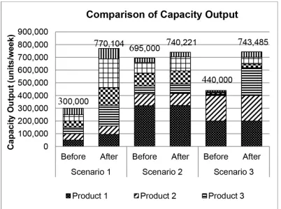
Figure 8 compares the capacity output before (demand from the marketing forecast) and after the implementation of CPGA (approximates optimum capacity level). Results from scenarios 1, 2, and 3 show higher capacity outputs compared with the capacity outputs before the implementation of CPGA with increments of 157%, 7%, and 69% for scenarios 1, 2, and 3, respectively.

7.1. Sensitivity analysis

The results were examined by fine-tuning the size of chromosome population N, probability of crossover (Pc), probability of mutation (Pm) and number of generation I to ensure that the near

optimal solution is reached. Performance was assessed with respect to the sensitivity test of the CPGA, at which near optimal solution is achieved.

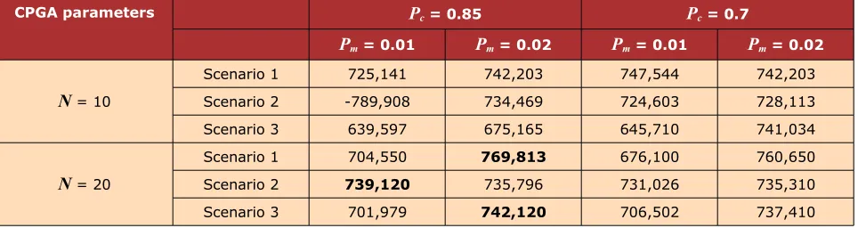
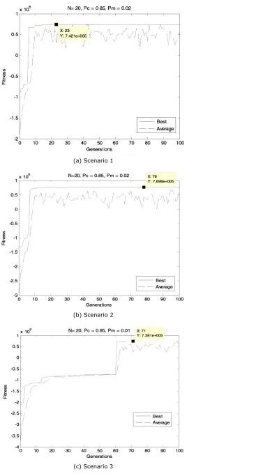
The generation number was fixed at 100 for all simulations. Table 7 indicates the effect of different CPGA parameters on fitness value. Each demand scenario has eight simulations with different parameter settings. A high population size with Pc = 0.85 and Pm = 0.02 produced the

highest fitness value in scenarios 1 and 3. Scenario 2 has the highest fitness value at lower mutation rate. From these simulations, the lower population size of Pc = 0.85 and Pm = 0.01

and resulted in worse fitness value. Table 7 shows the best solution for each scenario.

CPGA parameters Pc = 0.85 Pc = 0.7

Pm = 0.01 Pm = 0.02 Pm = 0.01 Pm = 0.02

N = 10

Scenario 1 725,141 742,203 747,544 742,203

Scenario 2 -789,908 734,469 724,603 728,113

Scenario 3 639,597 675,165 645,710 741,034

N = 20

Scenario 1 704,550 769,813 676,100 760,650

Scenario 2 739,120 735,796 731,026 735,310

Scenario 3 701,979 742,120 706,502 737,410

Table 7. CPGA simulation results

(a) Scenario 1

(b) Scenario 2

(c) Scenario 3

The comparison analysis shows that the run time was shorter and the results were better with higher mutation rate. For instance, Figure 10(a) and (b) in scenario 2 show performance graphs with different mutation rates but equivalent crossover rate and population sizes. Graphs in Figure 10(b), which has a higher mutation rate, shows that the curve started to increase at the earlier 35th generation compared with Figure 10(a), where graphs increased at the 66th generation.

(a)

(b)

Figure 10. The effects of mutation rate for (a) Pm = 0.01, (b) Pm = 0.02

increased at almost the same generation period, approximately at the 50th. However, the fitness value obtained was much higher when the population size was larger, which suggests that larger population size produces better solution compared to one with a smaller size. Under different crossover rate and similar mutation rate and population size, the performance graph patterns were almost similar (Figure 12(a) and (b)), which reflects that changes in crossover rate has no effect on the quality of solution.

(a)

(b)

(a)

(b)

Figure 12. The effects of crossover rate for (a) Pc = 0.7, (b) Pc = 0.85

8. Conclusion

determine the highest capacity output in all three scenarios. Significantly improved machine utilization was also achieved. The proposed approach can be easily extended to other more complex case scenarios, such as with longer routing operation of larger number of machine types.

The future works are promising in three areas. First, new practical elements are to be considered in the system including existing product inventory, different planning periods, profit margin and product prioritization. Second is to extend CPGA into actual application which requires software integration, human-machine interface design and management system. Finally, more efficient genetic algorithms, such differential evolution or other search algorithms can be explored, with the increase in problem complexity.

Acknowledgments

This research is sponsored fully by USM APEX grant (no: 910345) and FRGS (no: 6071276).

References

Abazari, A.M., Solimanpur, M., & Sattari, H. (2012). Optimum loading of machines in flexible manufacturing system using mixed-integer linear mathematical programming model and genetic algorithm. Computer & Industrial Engineering, 62, 469-478.

http://dx.doi.org/10.1016/j.cie.2011.10.013

Bajpai, P., & Kumar, M. (2010). Genetic Algorithm – an approach to solve global optimization problems. Indian Journal of Computer Science and Engineering, 1, 199-206. Available at: http://www.ijcse.com/docs/IJCSE10-01-03-29.pdf

Barták, R. (1999). Constraint programming: In pursuit of the holy grail. Proceedings of the Week of Doctoral Students (WDS99), 555-564.

Bilgin, S., & Azizoğlu, M. (2009). Operation assignment and capacity allocation problem in automated manufacturing systems. Computers & Industrial Engineering, 56, 662-676.

http://dx.doi.org/10.1016/j.cie.2007.04.003

Boussaïd, I., Lepagnot, J., & Siarry, P. (2013). A survey on optimization metaheuristics. Information Sciences, 237, 82-117. http://dx.doi.org/10.1016/j.ins.2013.02.041

Catay, B., Erengüç, S.S., & Vakharia, A.J. (2003). Tool capacity planning in semiconductor manufacturing. Computers& Operations Research, 30(9), 1349-1366.

Chen, S., & Smith, S.F. (1996). Commonality and genetic algorithms. Carnegie Mellon University, The Robotics Institute.

Chen, T.-L., & Lu, H.C. (2012). Stochastic multi-site capacity planning of TFT-LCD manufacturing using expected shadow-price based decomposition. Applied Mathematical Modelling, 36, 5901-5919. http://dx.doi.org/10.1016/j.apm.2012.01.037

Chiu, C., & Hsu, P. L. (2005). A constraint-based genetic algorithm approach for mining classification rules. IEEE Transactions on Systems, Man and Cybernetics, Part C: Applications and Reviews, 35(2), 205-220. http://dx.doi.org/10.1109/TSMCC.2004.841919

Geng, N., Jiang, Z., & Chen, F. (2009). Stochastic programming based capacity planning for semiconductor wafer fab with uncertain demand and capacity. European Journal of Operational Research, 198, 899-908. http://dx.doi.org/10.1016/j.ejor.2008.09.029

Guo, R.S., Chiang, D.M., & Pai, F.Y. (2007). A WIP-based exception-management model for integrated circuit back-end production processes. The International Journal of Advanced Manufacturing Technology, 33(11), 1263-1274. http://dx.doi.org/10.1007/s00170-006-0559-6

Haupt, R. L., & Haupt, S. E. (2004). Practical genetic algorithms. Wiley-Interscience.

Hsu, C.-I., & Li, H.-C. (2009). An integrated plant capacity and production planning model for high-tech manufacturing firms with economies of scale. International Journal of Production Economics, 118, 486-500. http://dx.doi.org/10.1016/j.ijpe.2008.09.015

Kovács, A., Váncza, J., Kádár, B., Monostori, L., & Pfeiffer, A. (2003). Real-life scheduling using constraint programming and simulation. Intelligent Manufacturing Systems, 213-218.

Li, G., Jiang, H., & He, T. (2014). A genetic algorithm-based decomposition approach to solve an integrated equipment-workforce-service planning problema. Omega. In pr e s s.

http://dx.doi.org/10.1016/j.omega.2014.07.003

Maleki-Dizaji, S., Nyongesa, H., & Khazaei, B. (2008). UPlanIT: an evolutionary based production planning and scheduling system. Nature Inspired Cooperative Strategies for Optimization (NICSO 2007), Studies in Computational Intelligence. Springer Berlin Heidelberg, 443-452.

Peng, Y., Lu, D., & Chen, Y. (2014). A constraint programming method for advanced planning and scheduling system with multilevel structured products. Discrete Dynamics in Nature and Society, Article ID 917685, 1-7. http://dx.doi.org/10.1155/2014/917685

Phruksaphanrat, B., Ohsato, A., & Yenradee, P. (2011). Aggregate production planning with fuzzy demand and variable system capacity base don Theory of constraints measures.

International Journal of Industrial Engineering: Theory Applications and Practice, 18(5), 219-231. Available at: http://journals.sfu.ca/ijietap/index.php/ijie/article/download/224/211

Qiu, R.G., Joshi, S., & Mcdonnell, P. (2004). An approach to regulating machine sharing in reconfigurable back-end semiconductor manufacturing. Journal of Intelligent Manufacturing,

15, 579-591. http://dx.doi.org/10.1023/B:JIMS.0000037709.69034.46

Rossi, F., Van Beek, P., & Walsh, T. (Eds.) (2006). Handbook of constraint programming, Vol. 2. Elsevier Science.

Schneider, T.R. (2002). A genetic algorithm for the identification of conformationally invariant regions in protein molecules. Acta Crystallogr. D Biol. Crystallogr, 58, 195-208. http://www.embl-hamburg.de/~tschneider/escet/jn0097.pdf

Swaminathan, J.M. (2000). Tool capacity planning for semiconductor fabrication facilities under demand uncertainty. European Journal of Operational Research, 120, 545-558.

http://dx.doi.org/10.1016/S0377-2217(98)00389-0

Tang, Y., Liu, R., & Sun, Q. (2014). Schedule control model for linear projects based on linear scheduling method and constraint programming. Automation in Construction, 37, 22-37.

http://dx.doi.org/10.1016/j.autcon.2013.09.008

Toomey, J.W. (1996). MRP II: planning for manufacturing excellence. Springer.

Ugwa, K.A. (2012). Mathematical modeling as a tool for sustainable development in Nigeria.

International Journal of Academic Research in Progressive Education and Development.

http://www.hrmars.com/admin/pics/867.pdf

Van Beek, P., & Chen, X. (1999). Cplan: A constraint programming approach to planning,

Proceedings of the national conference on artificial intelligence, John Wiley & Sons Ltd, 585-590. http://www.aaai.org/Papers/AAAI/1999/AAAI99-083.pdf

Wang, D.W., Fung, R.Y.K., & Lp, W.H. (2008a). An immune-genetic algorithm for introduction planning of new products. Computers and Industrial Engineering, 56, 902-917.

http://dx.doi.org/10.1016/j.cie.2008.09.036

Wang, K.J., Wang, S.M., & Chen, J.C. (2008b). A resource portfolio planning model using sampling-based stochastic programming and genetic algorithm. European Journal of Operational Research, 184, 327-340. http://dx.doi.org/10.1016/j.ejor.2006.10.037

You, F., Wassick, J.M., & Grossmann, I.E. (2009). Risk management for global supply chain planning under uncertainty: models and algorithms. AIChE Journal, 55, 931-946. Available at: http://egon.cheme.cmu.edu/Papers/RiskMgmtDow.pdf

Yusof, U.K., & Deris, S. (2010). Optimizing machine utilization in semiconductor assembly industry using constraint-chromosome genetic algorithm, IEEE International Symposium on Information Technology Conference Proceedings, 2, 601-606. Available at:

http://ieeexplore.ieee.org/stamp/stamp.jsp?arnumber=5561525

Zhang, R.Q. (2007). Research on capacity planning under stochastic production and uncertain demand. Systems Engineering - Theory & Practice, 27(1), 51-59. http://dx.doi.org/10.1016/S1874-8651(08)60006-X

Journal of Industrial Engineering and Management, 2014 (www. jiem. org)

Article's contents are provided on a Attribution-Non Commercial 3. 0 Creative commons license. Readers are allowed to copy, distribute and communicate article's contents, provided the author's and Journal of Industrial Engineering and Management's names are included.