minicourse

There are just a few workhorse models in macro:

I RBC / NK models

I Overlapping Generations (OLG) models

I Bewley / Huggett / Aiyagari (BHA) models

This leaves out a few substantial areas (search, heterogeneous firms), but it covers perhaps 95% of macro papers.

In fact, BHA models nest OLG models (I will show how later).

What does a typical BHA model look like?

Let’s look at the Aiyagari model for an example.

The Aiyagari model has two types of agents

I consumers/individuals/households

A unit measure of households

I Have a period utility function u(c), discount factor β I Consume c units of the consumption good

I Are endowed with 1 unit of time

I Have labor efficiencye ∈ E of the time endowment that evolves according to a Markov process.

I Are paid wagesw for each labor efficiency unit

⇒ earnings are we

I Have assetsa that have a return (1 +r−δ) where

I r is the rental rate on capital (a price)

I δis the depreciation rate on capital

I Choose assetsa0 subject to

The household problem is

V(a,e) = max

c,a0 u(c) +βEe0|eV(a 0_,e0₎

s.t. c +a0 =we+ (1 +r−δ)a c ≥0,a0 ≥a

Much of het agent macro is just variations on this theme:

I Adding death or other age-dependent features (OLG)

I Adding choices (e.g., labor, housing, education/human capital, job search, marriage, portfolio choice)

I Adding institutional details (e.g., Social Security, taxation)

I Adding limited commitment (what is a?)

I Adding firm profits (sometimes necessary)

I Adding aggregate shocks or additional heterogeneity

I z is total factor productivity (TFP) — constant

I K is stock of capital rented from households at rate r

I N is the aggregate amount of labor efficiency units hired at unit price w

I F is constant returns to scale (CRS)

I This ensures zero profits in equilibrium.

I If non-zero profits, need to think about firm ownership.

I F satisfies Inada conditions

The firm problem is

π= max

K≥0,N≥0zF(K,N)−rK −wN

Firm optimization⇒ equilibrium hasr =zFK and w =zFN.

To talk about any aggregates, we need to say whata ande are for the unit measure of households in the economy.

To properly set things up, the math becomes complicated.

For the most part we can think of a cdf “µ(a,e)” that says how many households have (a,e).

But formally one cannot sayµ(a,e), rather one must sayµ(A,E) whereA×E is in a product Borelσ-algebra over [a,∞) andE.

I The consumption good: c,Y

I The capital good: K,a,a0,a0−(1−δ)a

I The labor efficiency good: N,e.

(The price of capital is 1 here, but in general this need not be the case; e.g., see Greenwood, Hercowitz, Huffman, 1988, or Mendoza, 2010.)

Market clearing:

I Capital market clearing: K =R

adµ

I Labor (efficiency) market clearing: N =R edµ I Goods market clearing: Y =C +I where

I _{C is aggregate consumption}R _c(a,e)dµ.

I I is aggregate investmentR

A steady state recursive competitive equilibrium is

µ,V,c,a0,r,w,K,N such that

1. V solves the Bellman equation and c and a0 are optimal policies given r andw

2. Firms optimize, i.e., r andw are given by the marginal products.

3. Markets clear.

4. The distributionµ is invariant.

In general, ifµt is the distribution at time t, the distribution at

timet+ 1 is implicitly defined by the Markov process forE and the savings policy functiona0(a,e).

If everything is discrete withm(a,e) the m.d.f., then

mt+1(a0,e0) = X

a,e

1[a0 =a0(a,e)]F(e0|e)mt(a,e)

With measures, it’s much more complicated. But Theorem 9.13 in Stokey, Lucas, Prescott shows that Γ(A×E|a,e) defined by

Γ(A×E|a,e) =

F(E|e) if a0(a,e)∈A

0 if a0(a,e)∈/A

is a transition function (provideda0 is measurable).

Thenµt+1 is given by

µt+1(A,E) = Z

d(Γ(A×E|a,e)µt(a,e))

I V(a,e) is strictly increasing and concave ina.

I a0(a,e) is increasing ina — this holds with discretizeda.

I c(a,e) is increasing in a— this does not hold with discrete.

I The Bellman equation is a contraction mapping (modulusβ).

I To rule out Ponzi schemes, must always have some borrowing limita, even if it is arbitrarily large.

I Non-negative consumption imposes its own limit on debt, the

natural borrowing limit:

Specifically, one must have a0≥ −P∞

j=0(1 +r−δ)jw e where e = minE or c ≥0 would be violated with positive probability. (Note: where V(a,e) is well-defined depends on prices.)

I Equilibrium musthave β(1 +r−δ)<1, otherwise assets grow without bound.

I In eq., no upper bound ona0 is needed: a0(a,e)<afor a

large enough.

Precautionary savings, i.e., an increase ina0 in response to an increase in risk:

I This hinges on what Kimball (1990) call prudence,−u000/u00.

I If positive (i.e. u000>0), tend to have precautionary savings.

Three parts of solving the model:

1. Solving the household problem for a given r,w.

2. Solving for the invariant distribution

The simplest way to solve the h.h. problem: discretization.

Two aspects: discretizing the shocks and discretizing assets.

Suppose loge =ρloge−1+σε.

There are many methods to convert this to a Markov chain (e,F(e0|e)):

I Tauchen (1986)’s method

I Rouwenhorst method (Kopecky and Suen, 2010)

I Others

For discretizing the asset state space [a,∞), many options.

Pick an upper bounda, and then create #A points

{a:=a1, . . . ,a#A=:a}.

I Linear spacing (most common)

I Geometric spacing (to cluster around certain areas, use a)

⇒(ai+1−ai) =γ(ai −ai−1) for user-chosenγ.

Have to decide if also want a discretechoice space.

While if one restrictsa∈ A, one commonly a0∈ Arequires as well

⇒no interpolation.

But,a0∈[a,a] can also be done, ora0 ∈ A(forAsome other set).

V(a,e) = max

c,a0 u(c) +βEe0|eV(a 0

,e0)

s.t. c +a0 =we+ (1 +r−δ)a c ≥0,a0 ≥a

Write this like

V(i,j) = max

i0_{∈{1,...,#A}}u(c(i,j,i

0_{)) +β}X

j0

F(j0|j)V(i0,j0)

s.t. c(i,j,i0) =−a0+we+ (1 +r−δ)a c(i,j,i0)≥0,a0 ≥a

e =E_j

a=A_i

a0 =A_i0

for (i,j)∈ {1, . . . ,#A} × {1, . . . ,#E}.

Write this like

V(i,j) = max

i0_{∈{1,...,#A}}u(c(i,j,i

0_{)) +β}X

j0

F(j0|j)V(i0,j0)

s.t. c(i,j,i0) =−a0+we+ (1 +r−δ)a c(i,j,i0)≥0,a0 ≥a

e =E_j

a=A_i

a0 =A_i0

for (i,j)∈ {1, . . . ,#A} × {1, . . . ,#E}.

WhenV(i,j) is not well-defined, defineV(i,j) =−10100.

A couple things to note:

I For efficiency, W(i0,j) :=βP

j0F(j0|j)V(i0,j0) should be precomputed.

I The most efficient way is using matrix multiplication.

I IfF is stored in matrix π likeπ(j,j0) =F(j0|j), then W =βVπT.

I c(i,j,i0) on the other hand should not be precomputed — it is too large.

I The optimal policy function for this problem, call itg(i,j), gives the asset index.

I It is monotone in i, butc(i,j,g(i,j)) generally is not.

How to solve forV(i,j)?

Fix aj (i.e., loop over j), and letn=n0 = #A.

Defineπ(i,i0) =u(c(i,j,i0)) +W(i0).

Brute force does the following:

For eachi, computeπ(i,i0) for each i0 and save the best.

Simplest way: brute-force grid search.

do iE = 1 ,nE do iA = 1 , nA

! Set d e f a u l t u t i l i t y / p o l i c i e s

V ( iA , iE ) = -1 d 1 00 c ( iA , iE ) = -1 d0

api ( iA , iE ) = 1 ! set to 1 to g u a r a n t e e m o n o t o n i c i t y ! L o o p o v e r all iAp

do iAp = 1 , nA

if ( gA ( iAp ) < b o r r o w l i m ) c y c l e

c t m p = - gA ( iAp ) + gA ( iA ) * ( 1 d0 + r - d e p r e c ) + w *gE( iE ) if ( ctmp >0 d0 ) t h e n

v t m p = PU ( c t m p ) + CV ( iAp , iE )

! C o m p a r e u t i l i t y v e r s u s b e s t so far

if ( vtmp > V ( iA , iE )) t h e n V ( iA , iE ) = v t m p

c ( iA , iE ) = c t m p api ( iA , iE ) = iAp end if

One can go≈twice as fast using a small modification.

Becauseg(i−1)<g(i), can restrict the choice space for g(i) to

{g(i−1), . . . ,n}.

Simple monotonicity code:

do iE = 1 ,nE do iA = 1 , nA

! Set d e f a u l t u t i l i t y / p o l i c i e s

V ( iA , iE ) = -1 d 1 00 c ( iA , iE ) = -1 d0

api ( iA , iE ) = 1 ! set to 1 to g u a r a n t e e m o n o t o n i c i t y

! E x p l o i t the s i m p l e m o n o t o n i c i t y c o n d i t i o n

lb = 1

if ( iA >1) lb = api ( iA -1 , iE )

! L o o p o v e r iAp r e s t r i c t i n g the s e a r c h s p a c e

do iAp = lb , nA

! ... s a m e as b e f o r e

end do end do end do

i

i’

i

i’

Policy (g)

Search space

i

i’

Binary monotonicity (n=n’=100)

i

i’

Simple monotonicity (n=n’=100)

Can we do better than this? Yes, way better.

Supposeg(i) andg(i) are known for i <i.

Then for anyi ∈ {i, . . . ,i},g(i)∈ {g(i), . . . ,g(i)}.

Computingg(m) formthe integer midpointb(i+i)/2c, can use it

1. as an upper bound forg(i) with i ∈ {i+ 1,m−1}

This suggests thebinary monotonicity algorithm (Gordon and Qiu, 2018).

1. Definei = 1, i =n.

2. Solve forg(i) by checking all i0 ∈ {1, . . . ,n0}.

3. Solve forg(i) by checking all i0 ∈ {g(1), . . . ,n0}.

4. Ifi =i+ 1, STOP.

5. Let m=b(i +i)/2c and solve for g(m) checking

i0∈ {g(i), . . . ,g(i)}.

6. Go to step 4 twice, once redefining (i,i) = (i,m) and once (i,i) = (m,i).

i

i’

Binary monotonicity (n=n’=20)

i

i’

Simple monotonicity (n=n’=20)

Policy (g)

Search space

i

i’

Binary monotonicity (n=n’=100)

i

i’

i

i’

Binary monotonicity (n=n’=20)

i

i’

Simple monotonicity (n=n’=20)

Policy (g) Search space

i

i’

Binary monotonicity (n=n’=100)

i

i’

100 500 1000 2500 5000 10000 0

5 10 15 20 25 30

Convergence Time (Minutes)

Grid Size (n)

Minutes

including

1. simple concavity

2. binary concavity

3. two-state binary monotonicity

All the monotonicity can be combined with all the concavity and vice-versa.

Sufficient conditions for monotonicity are provided and very generally hold. Basically, need

1. increasing continuation utility

2. a concave flow utility function u(c)

3. a budget constraint like c =f(state,control) with

∂2_f

We’ll come back to some other techniques for solving the household problem.

But now let’s talk about how to compute the invariant distribution.

Imagine we are in the m.d.f. case having solved using discrete state and choice.

The distribution generally evolves like

mt+1(a0,e0) = X

a,e

1[a0 =a0(a,e)]F(e0|e)mt(a,e)

1. Let ˆm(a0,e0) = 0∀a0,e0

2. For eacha,e, do the following

ˆ

m(a0(a,e),e0) := ˆm(a0(a,e),e0) +mt(a,e)

Note that we are NOT usingF(e0|e) at this point. Conceptually, this corresponds to a “before shocks are realized” distribution between t and t+ 1.

3. Use matrix multiplication to set

mt+1= ˆmπ

whereπ(e,e0) =F(e0|e).

Note that for continuation utility we did W =βVπT, but here we use mt+1= ˆmπ. The former moves backwards in

Of course, you need to stop iterating at some point!

For the value function, a common stopping criterion is

|Vt+1−Vt|∞<10−xmax{|Vt|∞,1}.

Oftenx= 5,6,7,8.

The left hand side is the supnorm, andif you have a contraction mapping with modulusβ, it is guaranteed to satisfy

|Vt+1−Vt|∞

|Vt−Vt−1|∞

< β.

This is something you can (and should!) check. Violations = bugs!

One can check the supnorm for policies, too.

For the invariant distribution, a tight criterion like

|mt+1−mt|∞<10−x

Now you can solve the household problem and compute the invariant distribution.

The final step is finding the equilibrium prices,r,w.

SupposeY =zF(K,N) =zKαN1−α.

Thenr =zα(K/N)α−1,w =z(1−α)(K/N)α.

So,

K

N ⇒r,w ⇒a

0_{(a,e)⇒m(a,e)⇒} P

a,eam(a,e)

P

a,eem(a,e)

= K

LetG denote this mapping fromK/N to K/N.

Two ways to proceed:

1. Fixed point iteration: xt+1=G(xt)

Or, a “relaxed” version xt+1= (1−ξ)G(xt) +ξxt.

2. Root finding: f(x) :=G(x)−x, use a root-finding routine to find a zero of f.

(In Matlab,fzero works; but easy to code bisection in any language.)

Generally, I prefer root finding: Guaranteed to stop.

With everything discrete, an exact equilibrium does not exist.

to assess the model’s accuracy.

The Euler equation here, whenevera0 >a, is

u0(c(a,e)) =βEu0(c(a0(a,e),e0))(1 +r−δ)

This will generallynothold for the computed policies.

Consequently, we can define the EEE as

EEE(a,e) := log₁₀

1− u

0−1_(β

Eu0(c(a0(a,e),e0))(1 +r−δ))

c(a,e)

IfEEE(a,e) =−2, this means a $1 mistake in consumption is made for every $100 = 10−EEE(a,e) spent.

Here are some average Euler errors using discrete choice in BHA:

#A R

EEE(a,e)dµ(a,e) (conditional ona0 >a)

50 -1.1

100 -1.3

250 -2.0

500 -2.1

1000 -2.2

These are rather abysmal!

Note that, with brute force or simple monotonicity, doubling the # of gridpoints quadruples the cost. So the #A= 1000 point case is

400 timesmore costly than #A= 50.

deterministic case).15

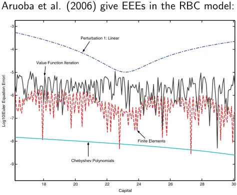
The maximum Euler error is useful as a measure of accuracy because it bounds the mistake that we are incurring owing to the approximation. Also, the literature on numerical analysis has found that maximum errors are good predictors of the overall performance of a solution.

Table 5presents the maximum Euler equation error for each solution method. We

can see how there are three levels of accuracy. Linear and loglinear, between!2 and

!3, the different perturbation and projection methods, all around!3:3, and value

function around!4:43. This table can be read as suggesting that, for this benchmark

calibration, all methods display acceptable behavior, with loglinear performing the worst of all and value function the best.

The second procedure to summarize Euler equation errors is to combine them with the information from the simulations to find the average error. This exercise is a generalization of the Den Haan–Marcet test where, instead of using the conditional expectation operator, we estimate an unconditional expectation using the population

18 20 22 24 26 28 30

-9 -8 -7 -6 -5 -4 -3 Capital Log10|Euler Equation Error|

Perturbation 1: Linear

Value Function Iteration

Chebyshev Polynomials

Finite Elements

Fig. 9. Euler equation errors atz¼0,t¼2=s¼0:007.

15_{0.065 corresponds to roughly the 99.5th percentile of the normal distribution given our}

parameterization. The interval for capital includes virtually 100 percent of the stationary distributions as computed in the previous subsection. Varying the interval for capital changes the size of the maximum Euler error but not the relative ordering of the errors induced by each solution method.

The Huggett model is almost the same as Aiyagari, but it is an endowment economy.

Rather than aggregate assets being capital, they are bond holdings.

Sow is exogenous,δ = 0, andr is the return that clears the bond marketRa0(a,e)dµ=B. (Usually,B = 0.)

(Terminology: lifecycle for PE crowd; OLG for GE crowd.) Consider the BHA model with only a few small tweaks:

V(a,s) = max

c,a0 u(c,s) +βρ(s)Es0|sV(a 0

,s0)

s.t. c +a0 =we(s) + (1 +r−δ)a+T(s)

c ≥0,a0 ≥a(s) Here,

I s as a vector of potentially many characteristics including

I age (I like this trick!)

I transitory and/or persistent and/or permanent shocks

I health, # children, married

I ρ(s) is a survival probability

I a(s) is a state dependent borrowing limit

I T(s) is accidental bequests.

Letj, a component ofs, denote age.

A few key facts for data / lifecycle models:

1. It should generally be solved by backwards induction.

2. How do we map consumption in the data to c in the model if there are N people in a households? Consumption equivalent scales, so e.g.

u(c,s) = p c

#hhmembers(j)

!1−σ

/(1−σ).

3. Usually e(s) = exp(φj +α+z+ε) where

I φj is a cubic polynomial in age from a regression on logwe.

I αis fixed for a persons life

I z follows an AR(1) process

I εis i.i.d.

the data (see, e.g., Kaplan, 2012) and be used to answer many interesting questions such as the implication of rising income inequality (documented e.g. in Heathcote, Perri, and Violante, 2010) or how much consumption insurance exists in the data (Kaplan and Violante, 2010, and see Blundell, Pistaferri, and Preston, 2008.)

One issue that has come up recently is a question of how many individuals areborrowing constrained.

Here, only constrained ifa0 = 0, and in the data there are not many like this.

A main drawback of the BHA models thus far: steady state.

Adding aggregate shocks leads to Krusell and Smith (1998).

(They also have a comparatively unknown 1997 paper.)

In the sequential equilibrium, the policy functions look like

c(et,zt) whereet andzt are the entire history of idiosyncratic and aggregate shocks.

One can use Stokey Luca Prescott to get an equivalence to

Conjecture: zt can be replaced withzt, µt.

Note thatzt, µt givesKt andNt, hence, rt andwt.

If one knewa0(·), one could then get µt+1 and hence all prices.

In general, this doesnotwork (Kubler and Schmedders, 2002).

Supposezt follows a Markov chain.

The recursive problem withz, µas the aggregate state is

V(a,e,z, µ) = max

c,a0 u(c) +βEz0,e0|z,eV(a 0

,e0,z0, µ0(z0))

s.t. c+a0=w(z, µ)e+ (1 +r(z, µ)−δ)a c ≥0,a0 ≥a

µ0(z0) = Γ(µ,z,z0)

Note that the prices are still marginal products, loosely,

r(z, µ) =zα(R

adµ/R

edµ)α−1 and

w(z, µ) =z(1−α)(R adµ/R edµ)α.

That still leaves a big problem: µis infinite dimensional!

Krusell and Smith propose replaceµwith a finite # of moments. Call the moments usedM.

Then the law of motion forM is specified as some exogenous, parametric function:

M0(z0) = ˜Γ(M,z,z0).

And, one has a mapping (either exogenous and parametric or determined by model structure) fromM to prices, r(z,M),

w(z,M).

The bounded rationality value function is

V(a,e,z,M) = max

c,a0 u(c) +βEz0,e0|z,eV(a 0

,e0,z0,M0(z0))

s.t. c+a0 =w(z,M)e+ (1 +r(z,M)−δ)a c ≥0,a0 ≥a

M0(z0) = ˜Γ(M,z,z0)

What can one use forM,Γ˜,r,w?

KS useM =K (just the first moment) with

logK0 =α0,z+α1,zlogK +ε.

(no dependence onz0 sinceK0 does not depend on it.)

The coefficients non-parametric dependence onz are very flexibile.

WithM =K,r(z,K) andw(z,K) are given in the natural way (withN a known function ofz).

The KS algorithm (for their setup):

1. Guess on α0,z, α1,z for eachz.

2. Solve the household problem given them.

3. Simulate:

I Useµt+1= Γ(µt,zt,zt+1) where{zt}are randomly drawn.

(Note: this is more accurate and not more costly than what KS originally proposed which is to also use Monte Carlo for the idiosyncratic shocks; see Young, 2009.)

I Compute time series{zt,Kt} and discard the firstT periods.

4. Run OLS regressions conditional (separately for each z) to get ˆ

α0,z,αˆ1,z.

5. Check if |αˆi,z−αi,z|is below some tolerance. If so, STOP.

6. Update theα0,z, α1,z using fixed point iteration:

How bounded is the rationality?

KS assess the forecast accuracy by looking at

1. The R2 on the 1-step ahead forecast,

2. the 1-step ahead forecast root mean square error (RMSE),

3. the maximum error on a 25-year ahead forecast

The key result in their paper—which has since shown to in many more complicated models—is that extremely accurate forecasts are obtained with onlyM =K. (No higher moments are needed.)

Why is the fit so good?

Ifa0(a,e;z, µ) wasexactly linear ina, then the K is a sufficient statistics forµ (in their model).

And, in fact, it is almost linear (and the slope does not depend much one.

Another reason in their model: The low earnings state hase = 0. So actually theira≥0 borrowing limit never binds, and the solution is always interior.

Tips:

I Be conservative withξ (i.e., useξ not too far from 1).

I To obtain convergence, important to fix the seed (or use a very long panel).

I The method is extremely flexible: As KS mention in footnote 10, a log-linear relationship is not needed. One can do semiparametric mappings such as α0,z,K∈[Ki,Ki+1),etc.

I You may have to be clever about the moments. E.g., with portfolio choice, you might want to include the equity premium as a “moment.”

Note that even the “plain-vanilla” Krusell-Smith starts becoming significantly more costly.

In BHA, #A ×#E states and #A choices.

In KS, states and choices #A ×#E ×#Z ×#Mand #Achoices.

Depending on the type of grid search and programming language, solving the KS model could take a few hours.

In quantitative models at the frontier, there may be two choice variables and more shocks, and time really becomes an issue.

One simple way to get more accuracy without much more cost is to make the choice space continuous.

Consider the case whereV(a,e) is given by a linear interpolant.

That is, fora∈[Ai,Ai+1]

V(a,e) = (1− a− Ai

A_i+1− A_i)V(Ai,e) +

a− Ai

A_i+1− A_iV(Ai+1,e)

Then note thatW(a0,e) =βEe0_|eV(a0,e0) is also given by its

linear interpolant:

W(a0,e) = (1− a

0_{− A}

i Ai+1− Ai

)W(A_i,e) + a

0_{− A}

i Ai+1− Ai

Then, the solution to this problem

V(a,e) = max

a0 u(c) +W(a 0

,e)

s.t. c+a0 =we+a(1 +r−δ),

a0∈[a,a] has either

1. a0(a,e) exactly atAi for somei OR

2. a0(a,e)∈(Ai,Ai+1) a solution to the FOC

u0(we+a(1 +r−δ)−a0) = W(Ai+1,e)−W(Ai,e)

A_i+1− A_i

In this case, one can solve for a0(a,e) as

a0 =we+a(1 +r−δ)−u0−1

W(A_i+1,e)−W(A_i,e)

Ai+1− Ai

(Note: precompute “whenever you can”, like theu0−1(·) term.)

Effectively, this doubles the number of choices.

But, the Euler errors can fall by two orders of magnitude!

Also, binary monotonicity is very efficient with this. (And it allows for non-concavities.) See the working paper on SSRN.

One can do similar things with other interpolation methods (though, the solution will not be closed form generally.)

A particular good one is Cai and Judd (EL, 2012): Simple, local interpolation formula that preserves shape.

When we computed the invariant distribution, we hada0 ∈ A.

What about with a continuous choice?

First note that, when using linearinterpolation, it can be interpreted as alotteryacross adjacent nodes:

W(a0,e) = (1−ω)W(A_i,e) +ωW(A_i+1,e)

whereω= a0−Ai

Ai+1−Ai

Using this interpretation, the nicest, simplest, and most cost efficient way is to distribute them as follows:

1. Let ˆm(a0,e0) = 0∀a0,e0

2. For eacha,e, do the following

I Locate ani such thata0(a,e)∈[Ai,Ai+1] (precompute!)

I Compute the weightωand distribute as

ˆ

m(Ai,e0) := ˆm(Ai,e0) + (1−ω) mt(a,e)

ˆ

m(Ai+1,e0) := ˆm(Ai+1,e0) +ω mt(a,e)

Note that we are NOT usingF(e0|e) at this point.

3. Use matrix multiplication to set

mt+1= ˆmπ

I Gornemann, Kuester, Nakajima R&R @ ECTA ; Dates to 2012 and uses standard methods with KS;

I McKay and Reis, ECTA 2016;

Projection methods with Reiter (2009) instead of KS.

I Kaplan, Moll, Violante, AER, 2018. Continuous time models.

In principal, you could do the GKN paper with what you know.

However, that is a very difficult computation.

The latter two papers are easier computationally, but you need to knowprojection methods.

Consider BHA with a natural borrowing limit.

The Euler equation is necessary and sufficient:

u0(c(a,e)) =βEe0_|eu0(c(a0(a,e),e0))(1 +r−δ) c(a,e) =we+a(1 +r−δ)−a0(a,e)

a0(a,e) =

K

X

k=0

αk,eTk(z(a))

wherez : [a,a]→[−1,1] monotonically and linearly and Tk is

some function you can look up on Wikipedia.

Then, if I told you whatα~ :={αk,e}k={0,...,K},e∈E, you could

evaluatea0(a,e) at any ain [a,a]× E.

You could then say whatc(a,e) =we+a(1 +r−δ)−a0(a,e) is.

Moreover, you could then say how wrong the Euler equation is,

R(a,e;~α) :=−u0(c(a,e)) +βEe0_|eu0(c(a0(a,e),e0))(1 +r−δ)

Let’s be concrete. Say{Tk} are the Chebyshev polynomials.

T0(z) = 1 T1(z) =z

Tk(z) = 2zTk−1(z)−Tk−2(z)

The linear functionz(a) = 2a_a−₋a_a −1.

To do an example, sayu= log, K = 1, a= 1,a=−1. Then

z(a) =a, and

a0(a,e) =

K

X

k=0

αk,eTk(z(a)) =α0,e+α1,ea,

Since

a0(a,e) =

K

X

k=0

αk,eTk(z(a)) =α0,e+α1,ea,

one has

c(a,e) =we+a(1 +r−δ)−a0(a,e) =we+a(1 +r−δ)−α0,e−α1,ea

Lastly,

R(a,e;~α)

:=−u0(c(a,e)) +βEe0_|eu0(c(a0(a,e),e0))(1 +r−δ)

=− 1

we+a(1−α1,e+r−δ)−α0,e

+βEe0_|e

1 +r−δ

c(α0,e+α1,ea,e0)

=− 1

we+a(1−α1,e+r−δ)−α0,e

+βEe0_|e

1 +r−δ

we0+ (α0,e+α1,ea)(1−α1,e0+r−δ)−α_0,e0

If the true policy function were linear, then there would exist anα~

such thatR(a,e;α~) = 0 uniformly.

In general, we can try to make the residualR close to zero.

For example, by solving min~αPa∈A,e∈ER(a,e;α~)2 using

This is an example of projection methods.

They are a very rich topic, and I spend weeks with my students doing them.

But ultimately, they convert infinite-dimensional objects (like

Let’s look at the continuous time version of the BHA model.

“Do not worry too much about your difficulties in mathematics, I can assure you that mine are still greater.” -Einstein

The reference you should look at is Achdou, Han, Lasry, Lions, Moll (R&R at ReStud). (Lions won the Fields Medal in 1994...)

In continuous time, the objective is to maximize the utility

E0

R∞

0 e

˙

at =yt+rat−ct.

The ˙at notation denotes a derivative with respect to time.

(Here, to be consistent with previous notation we should have

r−δ in place of r andwet in place ofyt, but it matters little.)

The borrowing limit is the same as before with

at ≥a.

Different processes foryt are possible:

I Poisson: yt ∈ {y1,y2}. Switch fromy1 to y2 with “intensity”

λ1 and vice-versa with λ2. Essentially, discrete time analog is p(y2|y1) =e1−λ1(see appendix B.1).

The recursive formulation of the continuous time problem is called a Hamilton-Jacobi-Bellman equation:

ρVj(a) = max

c u(c) +V

0

j(a)(y+ra−c) +λj(V−j(a)−Vj(a))

where−j means the opposite ofj (i.e.,j = 1 implies−j = 2 and vice-versa).

The curious thing here: Taking the FOC forc reveals flow consumption is trivially given as

u0(cj(a)) =Vj0(a)⇒cj(a) =u0−1(Vj0(a)).

Where does the borrowing constraint show up?

Where the borrowing constraint shows up is as a restriction that at

a=a, savings s :=y+ra−c must be positive.

Hence, one has as an additional equation that

yj +r a−cj(a)≥0⇔Vj0(a)≥u0(yj+r a).

The Euler equation is

(ρ−r)u0(cj(a)) =

u00(cj(a))cj0(a)(yj +ra−cj(a)) +λj(u0(c−j(a))−u0(cj(a)))

which uses the envelope conditionV_j0(a) =u0(cj(a)) and

differentiates it to getV_j00(a).

The Euler equation, with the SCBC

yj +r a−cj(a)≥0

characterizes the solution to the household problem.

Parameterizecj(a) = k=0αj,kTk(z(a)).

Construct a residual

R(a,j;α~) :=

−(ρ−r+λj)u0(cj(a)) +u00(cj(a))cj0(a)(yj +ra−cj(a)) +λju0(c−j(a))

+θmin{yj +r a−cj(a),0}2

Note thatθpenalizes violations of the borrowing constraint (so check deviations and increaseθ if too bad).

Minimize a weighted version of it, say

min

~ α

X

a∈A,j∈{1,2}

The Achdou et al. paper proposes a different projection method.

It is a special case of projection called finite elements, and it makes a lot of sense in continuous time.

But ultimately it is the same idea.

Ben Moll has many codes and notes on his website.

The Kaplan, Moll, Violante version of HANK follows fairly immediately from the Achdou et al. paper.

Two of the complications are (1) how are intermediate firm profits distributed and (2) what is the intermediate firms discount factor.

The McKay and Reis (2016) paper follows a different approach.

It is discrete time, and the computational trick there is it linearizes with respect to the distribution.

Here is a sketch of the Reiter (2009) approach.

Consider the KS model (without bounded rationality).

Suppose productivity evolves according to

logZt =ρlogZt−1+σεt.

The main idea is to solve forσ = 0—which is just a steady state, BHA economy—and then perturb/linearize it to obtain an approximation forσ >0.

Suppose we project the distribution as

m(a,e;~γt) = L

X

l=0

γl,e,tgk(a).

and the asset policy as

a0(a,e;α~t) = K

X

k=0

αk,e,tfk(a).

There are two equilibrium conditions that should be satisfied:

1. The Euler equation should hold and

Let the aggregate state be given byZt, ~γt.

Here,~γt gives the distribution (the state variable).

The distribution evolves in a known way given the policy choices and last period distribution:

~γt+1=Q(Zt+1,Zt, ~αt, ~γt).

Think of the Euler equation, but before taking the conditional expectation overZt+1:

0 =−u0(c(a,e;~αt,Zt;~γt))+ βEe0_|e,Zt,Zt

+1u 0

(c(a;e;α~t+1,Zt+1;~γt+1)(1 +r(Zt+1, ~γt+1)−δ)

(In steady state, we require~αt =α~t+1.)

So, equilibrium can be written as

EZt+1|Ztf(~αt+1, ~αt,Zt+1, ~γt+1,Zt, ~γt, σ) = 0

wheref stacks the distribution transition equation and Euler equation errors conditions.

This fits the form in Schmitt-Grohe and Uribe (2004) where

I [~αt] is a non-predetermined variable

I [Zt] is an exogenous predetermined variable I [γt] is an endogenous predetermined variable.

Practical considerations:

I Automatic differentiation (AD) is probably the best if you can use it. One IU student (Yongquan Cao) likes the AD Matlab code herehttps://sehyoun.com/codes.html.