Proposing New Methods to Enhance the Low-Resolution Simulated GPR Responses in the Frequency and Wavelet Domains

Int. J. Min. & Geo-Eng.

Vol.48, No.2, December 2014, pp.159-172.

159

Proposing New Methods to Enhance the Low-Resolution Simulated

GPR Responses in the Frequency and Wavelet Domains

Reza Ahmadi

, Nader Fathianpour

, Gholam Hossain Norouzi

1

Mining Engineering Department, Arak University of Technology, Arak, Iran 2

Mining Engineering Department, Isfahan University of Technology, Isfahan, Iran 3

School of Mining, College of Engineering, University of Tehran, Tehran, Iran

Received 3 Sep 2014; Received in revised form 18 Nov 2014; Accepted 22 Nov 2014 *Corresponding author: [email protected]

Abstract

To date, a number of numerical methods, including the popular Finite-Difference Time Domain (FDTD) technique, have been proposed to simulate Ground-Penetrating Radar (GPR) responses. Despite having a number of advantages, the finite-difference method also has pitfalls such as being very time consuming in simulating the most common case of media with high dielectric permittivity, causing the forward modelling process to be very long lasting, even with modern high-speed computers. In the present study the well-known hyperbolic pattern response of horizontal cylinders, usually found in GPR B-Scan images, is used as a basic model to examine the possibility of reducing the forward modelling execution time. In general, the simulated GPR traces of common reflected objects are time shifted, as with the Normal Moveout (NMO) traces encountered in seismic reflection responses. This suggests the application of Fourier transform to the GPR traces, employing the time-shifting property of the transformation to interpolate the traces between the adjusted traces in the frequency domain (FD). Therefore, in the present study two post-processing algorithms have been adopted to increase the speed of forward modelling while maintaining the required precision. The first approach is based on linear interpolation in the Fourier domain, resulting in increasing lateral trace-to-trace interval of appropriate sampling frequency of the signal, preventing any aliasing. In the second approach, a super-resolution algorithm based on 2D-wavelet transform is developed to increase both vertical and horizontal resolution of the GPR B-Scan images through preserving scale and shape of hidden hyperbola features. Through comparing outputs from both methods with the corresponding actual high-resolution forward response, it is shown that both approaches can perform satisfactorily, although the wavelet-based approach outperforms the frequency-domain approach noticeably, both in amplitude and shape of the outputted hyperbola response.

Keywords:forward modelling, fourier transform, Ground-Penetrating Radar (GPR), high resolution, wavelet transform.

160 1. Introduction

GPR is a high-resolution non-destructive geophysical technique which detects the convolved reflection of high-frequency (usually in the range of 1 MHz to more than 1 GHz) EM pulses caused by different subsurface in-homogeneity features, such as man-made artefacts, buried underground objects and natural subsurface geology. The main purpose of processing GPR data is to extract useful physical, structural and geometrical information about subsurface targets hidden in the raw data as a result of convolution. To achieve this goal it is necessary to obtain knowledge of the GPR system responses for various synthetic objects, which can be achieved using numerical forward modelling. Not only is the forward modelling process considered as the core engine of any practical inversion scheme, but also the simulated responses obtained via the forward modelling approach enable us to characterize the effect of different model parameters on expected GPR responses over corresponding objects.

To date, a number of different numerical forward modelling methods have been proposed and employed for simulating GPR responses, ranging from basic ray-tracing and one-dimensional (1D) transmission-reflection techniques [1] to more sophisticated finite-difference [2-8], finite-volume, Z-transform and discrete-element techniques (e.g., [9-11]) and their hybrids [12]. Although these methods are different in their methodology, they all attempt to simulate the propagation of the GPR wave from the surface downwards, with the emphasis on the interaction of the electromagnetic (EM) wave with the subsurface materials [13].

Among these forward modelling methods, the numerical finite-difference scheme has received most attention due to a number of advantages such as easier formulation, flexibility, ability to simulate and model complicated media, and reliable responses for known employed cases.

Only a few cases of applying wavelet transform in GPR data processing and enhancement have been reported. Delbò et al. (2000) applied a method based on the wavelet to reduce the noise and increase the signatures

in the GPR image, followed by use of a fuzzy clustering approach to identify the GPR signatures appearing as hyperbolas in GPR sectional images [14]. Strange et al. (2002) employed a GPR system to develop an algorithm to estimate the thickness of coal veins with a signal model representative of re-tuned GPR data. They used an adaptive filter extracted from pulse reflected off a metallic plane by wavelet to determine the distance to a target with an error of about 3 cm [15].

Rossini (2003) applied the wavelet transform and mathematical interpolation model to detect objects hidden in the subsoil [16]. Lian and Li (2011) applied an improved thresholding noise-suppression method based on wavelets to pre-process GPR data, followed by Hough transform to simulate the respective hyperbola response and determine the location of subsurface pipes. Finally, they classified simulated hyperbolas by the SVM method and obtained a correspondence between hyperbola classification results and pipe diameter [17].

In this study, two new methods have been used to improve the resolution and shape continuity of low-resolution simulated GPR responses in the frequency and wavelet domain. To achieve this goal, first the two-dimensional (2D) forward modelling based on finite-difference method is adapted for generating simulated GPR B-Scan data. Since any efficient inversion routine requires a fast forward modelling engine, this study will be aimed at developing fast forward modelling algorithms capable of being implemented in any inversion routine. Afterwards, the wavelet transform is employed to enhance the resolution of GPR images because this method is considered as an accurate and fast algorithm for such delicate interpolation. Finally, the results of the two methods are compared.

161 propagates. Dielectric permittivity (), magnetic permeability () and electrical conductivity () are the physical properties of the materials controlling the interaction of EM wave with different media. In most geological situations, the electrical properties tend to be the dominant factors controlling GPR responses. Since the magnetic permeability has trivial variations compared to the other properties then  and  are the most important physical property parameters in most cases in conventional GPR surveys.

In all cases one of the EM field components (generally electric field) is measured. The common way to display GPR data is to plot the returned signal amplitude against the delay time, which is called trace. In general the radargram obtained from profiling GPR data acquisition, as shown in Figure 1, contains a series of adjacent traces, and the resulting event in the image for most buried targets is a hyperbola. It is presumed that the detected reflected signal returned from the subsurface target is greater than the background signals.

Since GPR detects objects at a distance, resolution indicates how precisely the target geometrical parameters can be determined.

Resolution essentially breaks into depth and lateral resolution components when dealing with GPR data. In this study, the so-called lateral resolution, which accounts for angular or lateral response variations, is considered. The basic concepts of a typical GPR system are depicted in Figure 2.

Fig. 1. a) The procedure of GPR data acquisition by reflection-profiling (common-offset) mode over the buried object; b) a typical GPR radargram section in wiggle mode with the radar reflections showing a hyperbola pattern [18]

Fig. 2. Depth (a,c) and lateral (b,c) resolution components defined for GPR system (after [19]) (c)

(a) (b)

(a)

162 3. Application of FDTD method to simulate

GPR responses

In general the Maxwell’s equations and the associated initial and boundary conditions form the basis for studying EM field behaviour. The finite-difference numerical method is based on replacing the governing differential equations by their finite-difference approximations. To summarize, the whole finite-difference approach can be divided into three main stages: in the first step the space of the problem is discretized into a grid of nodes, followed by approximating the governing differential equations by finite-difference equivalents and finally solving the finite-difference equations imposed by appropriate initial and boundary conditions [20]. In order to avoid numerical divergency, the optimum spatial discretization interval of the finite-difference mesh should be at least ten times smaller than the wavelength of GPR antenna central frequency or the smallest dimension of the scatterer target. In other words, according to Equation (1) it should be one-fifth of the smallest wavelength in the transmitted pulse [20].

(1)



   _{x y} min

Equation (2) also calculates the time discretization step [21].

(2)

6

7 1 1

min min max t x y       

where min and min are the minimum values of

relative magnetic permeability and dielectric permittivity existing in the modelling grid, respectively.

In the finite-difference numerical modelling method, the EM fields are estimated at a number of grid nodes separated by x and y for a number of time steps (t). The most important parameters controlling the performance of numerical modelling are thus spatial discretization intervals and time steps. In general, lowering the spatial discretization resolution will result in greater accuracy at the cost of increased computation time and memory requirement. Therefore, it would be of great importance to reduce the computation time of GPR data forward modelling without losing accuracy.

4. Problems with the existing algorithms The most important drawbacks of the currently available numerical modelling codes (e.g., [3]) are the difficulties they present in model construction and the long computing time, in particular for lossy host media with high dielectric permittivity, where several hours are needed even with a modern and fast computer. Since any GPR data inversion algorithm needs a fast and reliable forward modelling engine, current research has been directed towards the development and implementation of optimized algorithms to reduce forward modelling time. As mentioned earlier, the GPR response for most buried objects (Fig. 1) appears as a hyperbola, meaning that the GPR signal traces reflecting the subsurface in-homogeneities show a time displacement in sequential traces. This time displacement allows taking the property of time-shifting in the Fourier transform frequency domain.

In order to increase the execution speed of the modelling while avoiding spatial aliasing or any possible numerical dispersion, the trace spatial intervals along the profile traverse are set to one-fifth of the target lowest dimension along the profile traverse strike. Optimizing this parameter significantly reduces the computation time. Obviously with this choice, the response resulting from GPR forward modelling appears fragmented and piecewise continuous, which is not desirable (here it is called low-resolution response).

5. Fourier domain approach to increase GPR forward responses

As outlined above, to increase the program

execution speed in the MATLAB

163 between two successive traces. Then, a number of desired synthetic traces are interpolated between two adjacent traces with the time displacement, applying the Fourier transform. In this study, in order to retain the curvature shape of the response a third-order 1-D interpolation scheme of type cubic spline is used between any two successive traces.

(3)





 

0

 

 F i t 

f t t e F

where t and t0 are time, i  1,  is angular

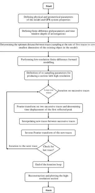
frequency and denotes the Fourier transform operation. These extra computations are very fast and take only a very short time, resulting in a more continuous trace-by-trace appearance in the GPR radargrams. The low-resolution piecewise fragmented appearance of the hyperbolic shape is also improved visually. This new GPR radargram is called high-resolution response. It should be mentioned that in order to increase the program execution, and to allow greater focus on the object response, the direct (air and ground) wave response in all traces is eliminated. Figure 3 shows the proposed flowchart for GPR high-resolution finite difference forward modelling algorithm.

The modified forward modelling program is designed in such a way as to provide both low-resolution and high-resolution outputs. Since most of the required time to compute each trace response goes to running all finite-difference equations in the forward modelling code, the application of Fourier transform and computation of trace interpolations in the Fourier domain leads to significant time reduction of about 12.5 times on the average models used in this study.

5.1. Validating the Fourier domain approach

In order to verify the performance of the proposed finite-difference forward modelling algorithm in terms of speed and resolution, GPR responses were generated for a number of hypothetical synthetic objects, especially single horizontal cylinders (representing a variety of pipes and circular Qanats), which are common in geotechnical investigations. To generate the above-mentioned targets, the GPR forward modelling code written by Irving and Knight

[3] in MATLAB was extended. By running the improved code, physical properties such as r, r and for the host medium and the target,

size of the GPR traversed cross-section, spatial discretization intervals and central frequency of the antenna were inputted first, followed by selecting one of the above-mentioned models.

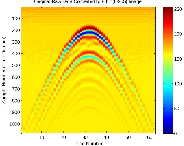
As an example, the two responses (low and high resolutions) of a single empty horizontal cylindrical object (filled by air) with a diameter of 1 m, embedded in a silty clay soil at a depth of 1 m (the distance to the top of the object) are illustrated in Figure 4. In the lower part of this figure the cross-section of the dielectric permittivity distribution is shown on the right and the conductivity distribution cross-section on the left (the dominant frequency of the EM wave is 250 MHz and the direction of profile traverse is perpendicular to the strike of the cylinder axis). The host medium physical properties are rh = 6 and h = 7 mS/m and the

cylindrical object has ro = 1 and o = 0 mS/m;

the values of magnetic permeability for the host medium and the target are the same and there is equal free space. The overall run time of forward modelling by the modified algorithm equals 5.15 minutes, compared to the 64.4 minutes needed for the code generated by Irving and Knight (2006). This shows a significant reduction in computational time by up to 12.5 times.

5.2. Results

164

Fig. 3. Flowchart of the proposed FDTD procedure to produce high-resolution GPR radargrams Iteration on successive traces

Iteration to the next trace

Start

Defining physical and geometrical parameters of the model and GPR system properties

Defining finite-difference grid parameters and time window (depth of investigation)

Definition of re-sampling parameters for producing a section with high-resolution Performing low-resolution finite-difference forward

modelling of final matrix (X,T ) with

Interpolating new traces between successive traces Fourier transform on two successive traces and determining

time displacement of the first reflected peak

Determining t he optimum distance between traces (sampling at the rate of five traces to cover smallest dimension of the existing object in the model)

Loop over traces

Inverse Fourier transform of the new traces

Check for last trace?

End of the iteration loop

Reconstruction and plotting the high-resolution section

with using all the traces

165

Fig. 4. Physical and geometrical parameters of an empty horizontal cylindrical model in the lower part. The GPR responses are shown in the upper part (low-resolution on the right and high-resolution on the left). The letters r, h and o stand for relative, host and object, respectively.

Original Raw Data Converted to 8 bit (0-255) Image

Trace Number

S

a

m

p

le

N

u

m

b

e

r

(T

im

e

D

o

m

a

in

)

10 20 30 40 50 60

100

200

300

400

500

600

700

800

900

1000

0 50 100 150 200 250

Fig. 5. Low-resolution GPR image (forward modelling response with 100 mm trace interspacing)

ro = 1

h = 7 mS/m

rh = 6

166

Original Raw Data with Direct Wave Removed

Trace Number

S

a

m

p

le

N

u

m

b

e

r

(T

im

e

D

o

m

a

in

)

20 40 60 80 100 120

100

200

300

400

500

600

700

800

900

1000

-15 -10 -5 0 5

x 10-3

Fig. 6. High-resolution GPR image (forward modelling response with 50 mm trace interspacing)

Trace Number

S

a

m

p

le

N

u

m

b

e

r

(T

im

e

D

o

m

a

in

)

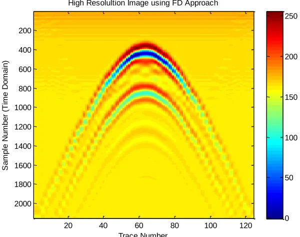
High Resolultion Image using FD Approach

20 40 60 80 100 120

200

400

600

800

1000

1200

1400

1600

1800

2000

0 50 100 150 200 250

Fig. 7. High-resolution GPR image (FD interpolated response with 50 mm trace interspacing)

6. Wavelet domain approach

6.1. Basis and applications of wavelet transforms

Wavelet theory, first proposed by Grossman and Morlet (1984), is a mathematical theory and analysis method which makes up the shortcomings of the Fourier transform [22]. In the field of signal processing, the most widely

167 variations of a signal, or detailed localized variations of an image. It can be shown that wavelet transform can localize features better than Fourier transform. In fact, the essence of wavelet analysis is multi-resolution analysis. Multi-resolution analysis is the decomposition of a signal or an image (such as GPR images) into sub-signals (or sub-images) of different resolution levels [23].

For example, Fourier transform of a sharp peak has a large number of coefficients because the basic functions of the Fourier transform are the cosine and sine functions, with constant amplitudes over the entire range, whereas the most energy of wavelet functions is concentrated in a small range and so is quickly damped. In fact, the theory of wavelets is the generalization of Fourier transforms and series theories, overcoming the pitfalls of Fourier analysis in local functioning and short-time behaviour modelling. Therefore, it can be used for a wide variety of fundamental signal processing tasks such as compression, removing noise, or enhancing recorded sounds or images, finding discrete points in signals, feature extraction from signals, analysis of different signals and in modelling and identification of systems [24]. Currently, there are several wavelet transforms in common use: Continuous Wavelet Transform (CWT), Discrete Wavelet Transform (DWT) and Fast Wavelet Transform (FWT).

There are some interpolation methods in the spatial domain that are specifically used in image processing applications. Such methods like pixel replication and bilinear interpolation techniques, usually up-sample an image without considering any structural details of the input image. These methods work well in simple and smooth regions but edges and some textures get blurred. As we know, the DWT procedure decomposes the image into four sub-bands (LL, LH, HL and HH) [23]. In wavelet-domain based techniques of image interpolation, the foremost challenge is to estimate unknown coefficients of three high-frequency sub-bands. The basic interpolation method in wavelet domain is Wavelet Zero-Padding (WZP). In this method a low-resolution image is multiplied with scaling factor S, which works as the top-left quadrant

(LL) of the final high-resolution image. In the other three quadrants of the high-resolution image (LH, HL and HH), zeros are padded [25]. In an application study, Temizel (2005) combined the directional cycle spinning property with WZP interpolation method [26].

In this paper the approach proposed by Naik and Patel (2013) has been adopted for producing single image super-resolution [25]. However, we have made a few modifications in the up-sampling and down-sampling procedure through using the bicubic spline of MATLAB instead of the image smoothing and sharpening routines of the Photoshop software. To prevent any unwanted high-frequency artefacts the method of error back-projection has been employed. Furthermore, in order to remove uncorrelated white noise from images, a wavelet-based denoising method is used.

6.2. Denoising radargrams in wavelet domain

In order to remove additive noise and at the same time maintain the most important details of images, denoising techniques are essential. The DWT-based denoising method offers useful capabilities, as wavelet transform contains large coefficients of images, which represent the detail of images at different scales. The LL sub-band contains the main information about the image while the main noises are included in the other three sub-bands; the maximum high-frequency noise is contained in HH [23,25].

168 The general denoising procedure used in this study involves three steps. The basic steps of the procedure include decomposing the image in the wavelet domain through choosing a suitable wavelet and level, computing the wavelet decomposition of the image at a corresponding level, estimating the appropriate threshold value for each level, applying soft thresholding to the detail coefficients, then carrying out wavelet reconstruction through computing the original approximation coefficients of level N and the modified detail coefficients of levels, iteratively. Not addressed here are the questions of how to choose the threshold and how to perform the thresholding (see [28]).

6.3. Down-sampling and up-sampling of the image

The flowchart of the algorithm for single image super-resolution proposed by Naik and Patel [25] was modified to enhance the entire procedure, as shown in Figure 8. As can be seen from this flowchart, measures of the stopping criterion based on the mean squared error (MSE) and the wavelet-based denoising procedure have been added to control the error back-projection process. All steps are summarized below.

In the first step, to gain the low-resolution image, a high-resolution image is taken and converted to a low-resolution image. To this goal can remove the arbitrary number of columns of the high-resolution image based on a given rule (e.g., every other column, etc.). The next step is up-sampling the image using bicubic interpolation algorithm. After up-sampling, due to the point spread function (PSF), the image can look a bit blurred. Gaussian filter works like a smoothing kernel, so applying a Gaussian smoothing filter to the image is the third step. In the next step, a stopping criterion based on MSE or maximum iteration is used. As in step 1, the image is down-sampled again (step 5). Steps 6 and 7 of the algorithm contain decomposing the image in the wavelet transform domain and denoising yielded HH sub-band respectively. By reversing the above procedure can achieve the reconstruction of the image, and is repeated until the image is fully reconstructed (step 8). In the next step of the algorithm (step 9), the

error is calculated between the original low-resolution image of step 1 and the down-sampled output image. Up-sampling the error is the most important step of the proposed algorithm (step 10). For reconstructing the super-resolution image, the error must be back-projected, and for that the error matrix must be up-sampled to correspond to the super-resolution image (step 11). This is done using the bicubic interpolation algorithm again. Finally, the error matrix generated in the previous step is added to the high-resolution image generated in step 8. The above procedure as shown in Figure 8 should be repeated until satisfactory results are achieved.

The final enhanced wavelet-based interpolation method to produce a high-resolution image is displayed in Figure 9. Based on the flowchart given in this figure, the original low-resolution GPR B-Scan image is primarily converted to a 256 level (8 bit) image. Next, the 2D SWT HAAR and DWT DB1 wavelets are employed to decompose the image of size m by n. The SWT procedure has the same dimension as the input image, while the DWT produces sub-bands with half the size of the input image. DWT is applied to the original image after applying the bicubic interpolation due to initial up-sampling. The reason for selecting applied types of wavelets is that the HAAR wavelet is simple as well as computationally fast compared to other kinds (e.g., Daubechies) that are well suited for complex irregular signals. However, other kinds of wavelet have also yielded similar results.

169

Fig. 8. Block diagram of the super-resolution algorithm (modified after [25])

No

Low-resolution image: I

Up-sampling the image: I

(n), n=0

Reconstruction error: E (n) = I

-I

Down-sampling: I

Back-projecting the error: I

(n+1) = E

(n) + I

(n)

Up-sampling the error: E

(n)

Gaussian filter: I

(n)

Pe rmit Max Ite r or Min

MSE

High-resolution image: I

(final)

Yes

Start

Finish

Stopping criterion (Max Iteration or Min MSE)

Wavelet decomposition of I

(n)

Denoising the HH component

170 6.4. Validating the wavelet-domain

approach

The same response of the cylindrical object is used as with the frequency-domain approach for interpolating the B-Scan image in spatial and wavelet domain. Therefore the image with 100 mm trace interspacing produced by finite-difference forward modeling (Fig. 5) has been employed as original low-resolution image. The true high-resolution image with 50 mm trace interspacing (Fig. 6) has also been applied as the reference for comparison.

Through an N level wavelet transforming the original image followed by updating the interpolated image via back projecting the

misfit errors in an iterative manner, required high-resolution image shown in Figure 10 has been achieved so that the trace interspacing has changed to 50 mm in final form. In this process the maximum level reached was 5 and the MSE measure was 5.54E-03.

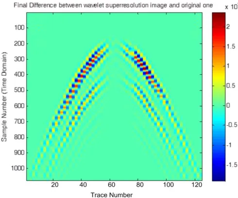
The main aim of this work is to show the lack of significant difference between the true high-resolution image and enhanced low-resolution image in wavelet transform. Figure 11 also plots the final difference between the original and wavelet super-resolution image. As can be seen from this figure, the image is completely symmetric.

Fig. 9. Proposed wavelet-based interpolation method (modified after [25])

Trace Number

S

a

m

p

le

N

u

m

b

e

r

(T

im

e

D

o

m

a

in

)

Final Wavelet Super-Resolution Image with Original Scale

20 40 60 80 100 120

100

200

300

400

500

600

700

800

900

1000

-15 -10 -5 0 5

x 10-3

171

Fig. 11. Final difference between the original and wavelet super-resolution image

7. Comparison

In the previous sections the applicable approaches for interpolating curvilinear features hidden in any image, including time-shifting in the frequency domain and interpolating in the wavelet transform domain, were applied to GPR B-Scan images. Based

on the visual comparison and misfit measures given in Table 1, it is found that although both approaches are capable of recovering hyperbola continuity hidden in GPR B-Scan images, the wavelet approach outperforms the FD approach in numerical precision (MSE measure in Table 1) and shape reconstruction.

Table 1. Comparison the performance of different methods based on MS E measure

Interpolating method FD approach Wavelet approach

MSE measure 9.36E-03 5.54E-03 8. Conclusion

The well-known pattern of GPR response of horizontal cylinder models, which is of hyperbolic shape, has been used for evaluating the performance of capable interpolating algorithms for post-processing GPR radargrams. Two entirely different algorithms have been proposed based on time shifting in the Fourier domain and filtering in the wavelet domain to interpolate adjacent traces. Through applying these approaches to the low-resolution GPR forward modelling response of a horizontal cylinder object and comparing with the actual high-resolution response, it is shown that through using the time-shifting theorem of Fourier transform and applying linear interpolation of the consecutive traces in the frequency domain, one can not only increase the lateral resolution of GPR forward responses along the profile traverses but also

reduce the forward modelling run-time significantly. The same response of the cylindrical object was employed for filtering in the wavelet transform domain, resulting in enhanced lateral resolution in addition to shape reconstruction.

References

[1] Goodman, D., (1994). Ground-Penetrating Radar simulation in engineering and archaeology. Geophys. v. 59, pp. 224-232.

[2] Karpat, E., Akır, M.C., Sevgi, L., (2009). Subsurface imaging, FDTD-based simulations and alternative scan/processing approaches . Microw. Opt. Techn. Let. v. 51, no. 4, pp. 1070-1075.

172 [4] Giannopoulos, A., (2005). Modeling ground

penetrating radar by GprMax. Constr. Build. Mater. v. 19, pp. 775-762.

[5] Cassidy, N.J., (2001). The application of mathematical modelling in the interpretation of Ground Penetrating Radar data. Ph.D. Thesis, Keele University.

[6] Chen, H.W., Huang, T.M., (1998). Finite- difference time- domain simulation of GPR data. J. Appl. Geophys. v. 40, pp. 139–163.

[7] Teixeria, F.L., Chew, W.C., Straka, M., Oristaglio, M.L., Wang, T., (1998). Finite- difference time- domain simulation of Ground Penetrating Radar on dispersive, inhomogeneous and conductive soils . IEEE. T. Geosci. Remote. v. 36, no. 6, pp. 1928–1937.

[8] Bergmann, T., Robertsson, J.O.A., Holliger, K., (1998). Finite- difference modelling of electromagnetic wave propagation in dispersive and attenuating media. Geophys. v. 63, no. 3, pp. 856–867.

[9] Yee, K.S., Chen, J.S., (1997). The finite- difference time- domain (FDTD) and the finite- volume time- domain (FVTD) methods in solving Maxwell’s equations. IEEE. T. Antenn. Propag. v. 45, no. 3, pp. 354–363.

[10] Roberts, R.L., Daniels, J.J., (1997). Modelling near-field GPR in three dimensions using the FDTD method. Geophys. v. 62, no. 4, pp. 1114–1126.

[11] Bourgeois, J.M., Smith, G.S., (1996). A fully three- dimensional simulation of a ground penetrating radar: FDTD theory compared with experiment. IEEE. T. Geosci. Remote. v. 34, pp. 36–44.

[12] Weedon, W.H., Rappaport, C.M., (1997). A general method for FDTD modelling of wave propagation in arbitrary frequency-dispersive media. IEEE. T. Antenn. Propag. v. 45, no. 3, pp. 401–409.

[13] Jol, H.M., (2009). Ground-Penetrating Radar theory and applications. First edition, Elsevier Science. 543 Pages.

[14] Delbò, S., Gamba, P., Roccato, D., (2000). A fuzzy shell clustering approach to recognize hyperbolic signatures in subsurface radar images. IEEE. T. Geosci. Remote. v. 38, no. 3, pp. 1447–1451.

[15] Strange, A., Chandran, V., Ralston, J., (2002). Signal processing to improve target detection using ground penetrating radar, Fourth

Australasian Workshop on Signal Processing and Applications (WOSPA), Brisbane, Australia.

[16] Rossini, M., (2003). Detecting objects hidden in the subsoil by a mathematical method . Comput. Math. Appl. v. 45, no. 1, pp. 299–307.

[17] Lian Fei-yu, Li Qing, (2011). Recognition method based on SVM for underground pipe diameter size in GPR map. Inform. Elect. Eng. v. 9, no. 4, pp. 403-408.

[18] http://mysite.du.edu/~lconyers/SERDP/ GPR2. htm

[19] Annan, A.P., (2001). Ground-penetrating radar workshop notes, Sensors and Software Inc. Mississauga, ON, Canada, 192 pages.

[20] Bergmann, T., Robertsson, J.O.A., Holliger, K. (1996). Numerical properties of staggered finite-difference solutions of Maxwell's equations for ground-penetrating radar modeling. Geophys. Res. Let. v. 23, no. 1, pp. 45-48.

[21] Georgakopoulos, S.V., Birtcher, C.R., Balanis, C.A., Renaut, R.A., (2002). Higher-order finite-difference schemes for electromagnetic radiation, scattering, and penetration, Part 1: theory. IEEE. Antenn. Propag. M., v. 44, pp. 134–142.

[22] Grossman, A., Morlet, J., (1984). Decomposition of Hardy functions into square integrable wavelets of constant shape. SIAM. J. Math. Anal. v. 15, no. 4, pp. 723-736.

[23] Walker, J.S., (2008). A primer on wavelets and their scientific applications, second edition, Chapman & Hall/CRC, Taylor & Francis Group.

[24] Gilbert, S., (1989). Wavelets and dilation equations: a brief introduction. SIAM Review, Published by: Soc. Ind. Appl. Math. v. 31, no. 4, pp. 614-627.

[25] Naik, S., Patel, N., (2013). Single image super resolution in spatial and wavelet domain. Int. J. Multi. Appl. (IJMA), v. 5, no. 4, pp. 23-32.

[26] Temizel, A., Vlachos, T., (2005). Image resolution up scaling in the wavelet domain using directional cycle spinning. J. Electron. Let. v. 41, pp. 119–121.

[27] Misiti, M., Misiti, Y., Oppenheim, G., Poggi, J.-M. (eds) (2007). Frontmatter, in wavelets and their applications, ISTE, London, UK. doi:10.1002/9780470612491.fmatter