Wind-farm layout optimisation using a hybrid Jensen–LES approach

(1)

doi:10.5194/wes-1-311-2016

Wind-farm layout optimisation using a hybrid

Jensen–LES approach

Vahid S. Bokharaie, Pieter Bauweraerts, and Johan Meyers

KU Leuven, Department of Mechanical Engineering, Celestijnenlaan 300A, B3001 Leuven, Belgium Correspondence to:Johan Meyers ([email protected])

Received: 28 April 2016 – Published in Wind Energ. Sci. Discuss.: 11 May 2016 Revised: 29 September 2016 – Accepted: 27 October 2016 – Published: 5 December 2016

Abstract. Given a wind farm with known dimensions and number of wind turbines, we try to find the optimum

positioning of wind turbines that maximises wind-farm energy production. In practice, given that optimisation has to be performed for many wind directions, and taking into account the yearly wind distribution, such an optimisation is computationally only feasible using fast engineering wake models such as the Jensen model. These models are known to have accuracy issues, in particular since their representation of wake interaction is very simple. In the present work, we propose an optimisation approach that is based on a hybrid combination of large-eddy simulation (LES) and the Jensen model; in this approach, optimisation is mainly performed using the Jensen model, and LES is used at a few points only during optimisation for online tuning of the wake-expansion coefficient in the Jensen model, as well as for validation of the results. An optimisation case study is considered, in which the placement of 30 turbines in a 4 km by 3 km rectangular domain is optimised in a neutral atmospheric boundary layer. Optimisation for both a single wind direction and multiple wind directions is discussed.

1 Introduction

Wind turbines are often clustered together in wind farms to save the cost of land and cabling. However, aerodynamic interactions between the turbines in the form of so-called wakes (low-speed regions) that form behind wind turbines lead to power reductions in “waked” turbines of up to 50 % compared to a lone-standing wind turbine in undisturbed flow (Barthelmie et al., 2010). These interactions are very important when considering the topological placement of wind turbines in large wind farms.

In order to optimally design wind-farm layout, models are necessary that accurately predict the aerodynamic turbine– wake interaction effects. Such models need to be very fast, as wind-farm design optimisation needs to consider the full spectrum of wind directions over a wind farm’s operational lifetime, thus requiring many thousands of model evalu-ations. Moreover, wind-farm design is a multidisciplinary problem in which the aerodynamic wake-interaction model is only one of the models, next to turbine load models, lifetime analysis, economic investment models, etc. (see, e.g., Zaaijer, 2013). Today, the wake model that is most used

is the Jensen model (Jensen, 1983; Katic et al., 1986). It is a simple and fast model, but it is known to be inaccurate when looking at individual power predictions of turbines in various waked conditions (Barthelmie et al., 2009; Gaumond et al., 2014; Niayifar and Porté-Agel, 2015). Layout optimi-sation of wind farms using fast wake models has been inves-tigated in numerous studies (Marmidis et al., 2008; Emami and Noghreh, 2010; Kusiak and Song, 2010; González et al., 2010; Saavedra-Moreno et al., 2011; Du Pont and Cagan, 2012; Chowdhury et al., 2012; Samorani, 2013; Chen et al., 2013b). However, the accuracy of such optimisation results has always remained a concern in view of the limited relia-bility of wake models, and this has recently led to a renewed interest in the formulation of accurate but fast wake models (Stevens et al., 2015; Niayifar and Porté-Agel, 2015).

In the last five years, the detailed simulation of wind-farm– atmospheric-boundary-layer interaction and turbine wake in-teractions based on high-fidelity simulation tools such as large-eddy simulation (LES) have become very popular (see, e.g., Meyers and Meneveau, 2010; Calaf et al., 2010; Yang et al., 2012; Meyers and Meneveau, 2013; Wu and Porté-Agel,

(2)

2013; Allaerts and Meyers, 2015), leading to many new in-sights into the flow physics of wind farms. Given known and constant meteorological conditions, these types of models provide a detailed time-resolved prediction of the turbulent flow in a wind farm with resolution of spatial flow structures in the order of 20 m and temporal fluctuations in the order of 10 s. Although it is computationally infeasible in LES of wind farms to resolve all the detailed flow physics, such as the turbine blade-boundary layers (with length scale below a millimetre), these models do lead to quite accurate predic-tions of wakes and wake merging when compared to wind-tunnel and field experiments (Porté-Agel et al., 2011; Wu and Porté-Agel, 2013; Munters et al., 2016a). Unfortunately, LES of wind farms requires supercomputing and simulation times that are several hours to days for one single atmospheric con-dition. Hence, these models are not useful for layout optimi-sation purposes.

In the current work, we investigate a hybrid approach in which the Jensen model is used during optimisation, but we use LES to gradually adapt the Jensen model and verify the optimisation results. To this end, the wake-expansion coeffi-cient in the Jensen model is iteratively fitted based on LES. In itself, tuning of the wake-expansion coefficient (e.g. to ex-periments) is quite common, but it is well known that the coefficient depends on atmospheric conditions and farm lay-out, and it may also best depend on streamwise distance into the farm (Stevens et al., 2015). Therefore, a coefficient that is tuned a priori will not fit all possible scenarios that are en-countered during layout optimisation of a wind farm over its relevant range of atmospheric conditions. In a hybrid Jensen– LES approach, it is possible to adapt the coefficient a posteri-ori during optimisation depending on layout, wind direction, etc. The main focus of the current work is on the formula-tion of an approach that is computaformula-tionally feasible, given the very high costs of performing LES (even in a hybrid Jensen– LES optimisation). We demonstrate the proposed methodol-ogy on a moderately sized wind farm of 30 turbines in a 4 km by 3 km farm area.

This paper is organised as follows. In Sect. 2 the mathe-matical formulation for the optimisation problem is stated, and the simulation models (both Jensen and LES) and the optimisation methodology are introduced. In Sect. 3, results are presented. First, the different steps in the algorithm are highlighted for a single wind-direction optimisation case in Sect. 3.1–3.3. Subsequently, in Sect. 3.4, some results for op-timisation with multiple wind directions are discussed. Fi-nally, conclusions are presented in Sect. 4.

2 Problem description and methodology

In Sect. 2.1, the optimisation problem description is intro-duced. Subsequently, the Jensen model is briefly reviewed in Sect. 2.2. The LES simulation environment is discussed in

Sect. 2.3, and finally the hybrid Jensen–LES approach and the optimisation method are presented in Sect. 2.4.

2.1 Problem description

Consider a set ofN_tturbines that are to be placed in a fixed

domain. Given constant atmospheric conditions and wind

direction (parameterised in a vectorµ), the average power

output of a turbine at positionxiin the wind farm is

Pi(xi,µ)= 1

T

Z

0

Pi(xi, t,µ)dt, (1)

wherePi(xi, t,µ) corresponds to the instantaneous power output of the turbine (given atmospheric conditions µ),

which is subject to turbulent wind fluctuations, and T is a

time averaging window that is sufficiently long to average out the turbulence effects. Note that the Jensen model (see Sect. 2.2) directly predictsPi of turbines in a wind farm, while, for example, experimental measurements as well as results from LES (see Sect. 2.3) yieldPi(xi, t,µ) and thus explicitly require the above time averaging.

The optimisation problem that we consider is formulated as follows:

maximise

xi Z

XNt

i=1Pi(xi,µ)fp(µ)dµ subject to xi ∈, ∀i∈ {1,· · ·, Nt}

kxi−xjk2≥dmin ∀i, j∈ {1,· · ·, N_t}, i6=j,

(2)

whereis the wind-farm domain in which turbines can be

freely placed andfp(µ) is the joint probability density

func-tion of atmospheric condifunc-tions µ over which optimisation

needs to be carried out (e.g. the yearly wind-direction dis-tribution, atmospheric stability class). Finally,d_minis a

con-straint on the minimum distance between turbines. In theory, the minimum distance between turbines is 1.0D(withDthe

rotor diameter). In the current study, we will consider ad_min

of 2.0Dfor all optimisation cases.

The solution of the above optimisation problem requires a model forPi(xi,µ). This is discussed next in Sect. 2.2 for the Jensen model and in Sect. 2.3 for the LES model. To solve the above optimisation problem, we use the cross-entropy op-timisation method (De Boer et al., 2005; Rubinstein, 1999) in combination with a hybrid Jensen–LES model as discussed in Sect. 2.4. Finally, note that, for ease of notation, we drop

µas an argument inPi. In fact, the conditionsµ(e.g. wind direction, turbulence intensity) are implicity contained on the set-up and boundary conditions of the respective models be-low.

2.2 The Jensen wake model

(3)

The model commences by assuming that each turbine gen-erates a radially and azimuthally uniform wake that linearly expands with downstream distance from the turbine. Using simple mass conservation, this allows the velocity deficit generated by turbineito be described as

1Ui(si)=U∞ 1−p

1−C_T,i (1+k_wsi/R)2

, si>0, (3)

whereC_T,iis the turbine thrust coefficient andsi=(x−xi)· e_fis the downstream axial distance from the turbine, ande_f

the unit vector in the mean-flow direction. Obviously,si >0. Upstream of a turbine, its own generated wake has a ve-locity deficit 1Ui=0. Furthermore,kw is the linear wake-expansion coefficient, andRis the rotor radius. Correlations

exist that relate k_w to the incoming atmospheric boundary

layer; for example (Lissaman, 1979; Frandsen, 1992)

k_w= u∗

U∞

= κ

ln(z_h/ z₀) (4)

is commonly used, withκ the von Kármán constant,z_h the

turbine hub height, andz₀andu∗the surface roughness and friction velocity of the incoming atmospheric boundary layer. Note that, in the current study, we will use LES to adaptk_win

our optimisation procedure as discussed in Sect. 2.4. Finally note that the wake expansion is vertically restricted by the ground once the wake radius grows larger than the turbine hub height. However, the ground is not directly modelled, but instead mirror turbines are added below the ground, with wakes that are included in the wake-merging model (Lis-saman, 1979) (see below).

In order to estimate the power outputPi, the turbine’s in-coming mean velocity is required. It is modelled asUi,in=

U∞−1Ui,in, withU∞the wind-farm inflow velocity at hub height and1Ui,inthe upstream velocity deficit experienced by turbinei. The deficit1Ui,inis heuristically modelled by quadratically adding upstream wake deficits as follows:

1Ui,in=



 X

j∈Si

(1Uj(sij))2





1/2

. (5)

HereSi is the set of all upstream turbines that have a wake that geometrically intersects with turbineiandsij is the dis-tance along the wind direction between turbine i andj. In

order to include the effect of the ground on wake develop-ment, mirror turbines (below the ground) are added to the set

Si for each turbine whose wake is restricted by the ground. It is furthermore possible that wakes only partially overlap, in which case the rotor area of the inflow turbine is split into regions with different overlaps. More details on the approach can be found in Rathmann et al. (2007).

Once the turbine inflow velocitiesUi,inare determined, the

power per turbine is calculated as

Pi(xi)= 1

2CP,iρUi,3in, (6)

whereCP,i is the wind turbine’s power coefficient. For an ideal turbine, CP,i follows from axial momentum theory from, i.e.

C_P,i=1

2CT,i[1− 1−CT,i

1/2

]. (7)

For a real turbine,C_P,ican be expressed as a function ofCT,i and wind speed, using either a mapping specific to the turbine or blade-element momentum theory, and this can be straight-forwardly used in the Jensen model. In the current study, we will simply use above ideal relationship, as our main focus is on the development and demonstration of the hybrid Jensen– LES approach, and not so much on the specifics of the se-lected turbine model.

2.3 Large-eddy simulation environment and simulation set-up

Simulations are performed using SP-Wind, developed at KU Leuven (Meyers and Meneveau, 2010, 2013; Allaerts and Meyers, 2015; Goit and Meyers, 2015; Munters et al., 2016a). SP-Wind solves the filtered incompressible Navier– Stokes equations, which are given by

∇ ·

eu=0 (8)

∂_eu

∂t +eu· ∇eu= −

1

ρ∇pe+ ∇ ·τM−f, (9)

whereeu(x, t)= [eu1,eu2,eu3]is the resolved velocity field,pe

is the pressure field, and τ_M is the sub-grid-scale (SGS)

model. We use a standard Smagorinsky model (Smagorin-sky, 1963) with Mason and Thomson’s wall damping (Mason and Thomson, 1992) to model the SGS stress. Furthermore, −f represents the forces (per unit mass) introduced by the

turbines on the flow. In LES of wind-farm boundary layers, this turbine-induced force is commonly modelled using an actuator-disc model (ADM), as full meshing of the turbine blades and geometry leads to computational grids that are too large for current-day computers. Expressed for turbinei,

this force corresponds to (Meyers and Meneveau, 2010; Goit and Meyers, 2015):

f(i)=1 2C

0

T,iVb_i2

which are given by

∇ ·

u

e

= 0

(8)

∂

u

_e

∂t

+

u

e

· ∇e

u

=

−

1 ρ

∇e

p

+

∇ ·

τ

M

−

f

(9)

where

u

e

(

x

, t

) = [

u

e

1

,

u

e

2

,

u

e

3

]

is the resolved velocity field,

p

e

is the pressure field, and

τ

M

is the subgrid-scale (SGS) model.

We use a standard Smagorinsky model (Smagorinsky, 1963) with Mason & Thomson’s wall damping (Mason and Thomson,

5

1992) to model the SGS stress. Furthermore,

₋

f

represents the forces (per unit mass) introduced by the turbines on the flow.

In LES of wind-farm boundary layers, this turbine-induced force is commonly modelled using an actuator-disk model (ADM),

as full meshing of the turbine blades and geometry leads to computational grids that are too large for current-day computers.

Expressed for turbine

i

, this force corresponds to (Meyers and Meneveau, 2010; Goit and Meyers, 2015):

f

(i)

=

1

2 C

T,i0

V

b

i2

R

i(

x

)

e

⊥

i

= 1

···

N

t

,

(10)

10

where

e

_⊥

represents the unit vector perpendicular to the turbine disk, and

R

i(

x

)

is a geometrical smoothing function that

distributes the uniform surface force of the turbine over surrounding LES grid cells, with

R

_Ω

R

i(

x

)

d

x

0

=

A

and

A

the turbine

disk area. Moreover,

V

b

i

is the disk-averaged turbine velocity, and

C

T,i0

is the disk-based thrust coefficient. Unlike the

conven-tional thrust coefficient

C

T

(used in the Jensen model) which is based on undisturbed velocity far upstream of a turbine,

C

T,i0

is defined using the velocity at the turbine-disk. It results from integrating lift and drag coefficients over the turbine blades,

15

taking design geometry and flow angles into account (cf. Appendix A in Goit and Meyers, 2015 for a detailed formulation).

Based on axial momentum theory, we have (Calaf et al., 2010):

C

T

=

C

0 T

(1 +

C

_T0

/

4)

2

(11)

which provides a direct relation between the thrust coefficient used in the Jensen model, and the disk-based thrust coefficient

used in the LES model. Finally, given the velocity field

u

e

(

x

, t

)

from a LES, the average power output for turbine

i

is determined

20

from

P

i(

x

i) =

1 T

T

Z

0

ZZZ

f

(i)

· u

e

d

x

d

t.

(12)

In Figure 1 a typical snapshot of a horizontal velocity field

_e

u

1

(

x

, t

)

is shown, including an outline of the simulation domain

that is considered in the current study. The main domain size is

L

y

×

L

x

×

L

z

= 8

.

0 ×

6 .

0 ×

1 .

0 km

3

, where

x

is always the

main flow direction, and

z

is the vertical direction. The wind-farm is inserted in a subdomain

Ω = 4

.

0 km

×

3 .

0 km (also marked

25

on the figure). At

z

= 0

a classical high-Reynolds-number wall-stress boundary condition is used (Moeng, 1984; Bou-Zeid

et al., 2005), which is parametrized by the ground surface roughness

z

0

, for which we use

z

0

= 0

.

1 m. At

z

=

L

z

a symmetry

condition is used, and in the

y

direction, periodic boundary conditions are used. Finally, at

x

= 0

an inflow boundary condition

is used.

The inflow is generated in a separate precursor simulation (also shown in Figure 1), which employs shifted periodic boundary

30

conditions to avoid artificial spanwise locking of the typical low-speed streaks observed in boundary layers (cf. Munters et al.,

5

i(x)e⊥; i=1· · ·Nt, (10)

wheree⊥represents the unit vector perpendicular to the tur-bine disc, and

which are given by

∇ ·

u

e

= 0

(8)

∂

u

_e

∂t

+

u

e

· ∇e

u

=

−

1 ρ

∇e

p

+

∇ ·

τ

M

−

f

(9)

where

u

e

(

x

, t

) = [

u

e

1

,

u

e

2

,

u

e

3

]

is the resolved velocity field,

p

e

is the pressure field, and

τ

M

is the subgrid-scale (SGS) model.

We use a standard Smagorinsky model (Smagorinsky, 1963) with Mason & Thomson’s wall damping (Mason and Thomson,

5

1992) to model the SGS stress. Furthermore,

₋

f

represents the forces (per unit mass) introduced by the turbines on the flow.

In LES of wind-farm boundary layers, this turbine-induced force is commonly modelled using an actuator-disk model (ADM),

as full meshing of the turbine blades and geometry leads to computational grids that are too large for current-day computers.

Expressed for turbine

i

, this force corresponds to (Meyers and Meneveau, 2010; Goit and Meyers, 2015):

f

(i)

=

1

2 C

T,i0

V

b

i2

R

i(

x

)

e

⊥

i

= 1

···

N

t

,

(10)

10

where

e

_⊥

represents the unit vector perpendicular to the turbine disk, and

R

i(

x

)

is a geometrical smoothing function that

distributes the uniform surface force of the turbine over surrounding LES grid cells, with

R

_Ω

R

i(

x

)

d

x

0

=

A

and

A

the turbine

disk area. Moreover,

V

b

i

is the disk-averaged turbine velocity, and

C

_T,i0

is the disk-based thrust coefficient. Unlike the

conven-tional thrust coefficient

C

T

(used in the Jensen model) which is based on undisturbed velocity far upstream of a turbine,

C

T,i0

is defined using the velocity at the turbine-disk. It results from integrating lift and drag coefficients over the turbine blades,

15

taking design geometry and flow angles into account (cf. Appendix A in Goit and Meyers, 2015 for a detailed formulation).

Based on axial momentum theory, we have (Calaf et al., 2010):

C

T

=

C

_T0

(1 +

C

0 T

/

4)

2

(11)

which provides a direct relation between the thrust coefficient used in the Jensen model, and the disk-based thrust coefficient

used in the LES model. Finally, given the velocity field

u

e

(

x

, t

)

from a LES, the average power output for turbine

i

is determined

20

from

P

i(

x

i) =

1 T

T

Z

0

ZZZ

f

(i)

· u

e

d

x

d

t.

(12)

In Figure 1 a typical snapshot of a horizontal velocity field

u

_e

1

(

x

, t

)

is shown, including an outline of the simulation domain

that is considered in the current study. The main domain size is

L

y

×

L

x

×

L

z

= 8

.

0 ×

6 .

0 ×

1 .

0 km

3

, where

x

is always the

main flow direction, and

z

is the vertical direction. The wind-farm is inserted in a subdomain

Ω = 4

.

0 km

×

3 .

0 km (also marked

25

on the figure). At

z

= 0

a classical high-Reynolds-number wall-stress boundary condition is used (Moeng, 1984; Bou-Zeid

et al., 2005), which is parametrized by the ground surface roughness

z

0

, for which we use

z

0

= 0

.

1 m. At

z

=

L

z

a symmetry

condition is used, and in the

y

direction, periodic boundary conditions are used. Finally, at

x

= 0

an inflow boundary condition

is used.

The inflow is generated in a separate precursor simulation (also shown in Figure 1), which employs shifted periodic boundary

30

conditions to avoid artificial spanwise locking of the typical low-speed streaks observed in boundary layers (cf. Munters et al.,

5

i(x) is a geometrical smoothing function that distributes the uniform surface force of the turbine over surrounding LES grid cells, withR

which are given by

∇ ·

u

e

= 0

(8)

∂

u

_e

∂t

+

u

e

· ∇e

u

=

−

1 ρ

∇e

p

+

∇ ·

τ

M

−

f

(9)

where

u

e

(

x

, t

) = [

u

e

1

,

u

e

2

,

u

e

3

]

is the resolved velocity field,

p

e

is the pressure field, and

τ

M

is the subgrid-scale (SGS) model.

We use a standard Smagorinsky model (Smagorinsky, 1963) with Mason & Thomson’s wall damping (Mason and Thomson,

5

1992) to model the SGS stress. Furthermore,

₋

f

represents the forces (per unit mass) introduced by the turbines on the flow.

In LES of wind-farm boundary layers, this turbine-induced force is commonly modelled using an actuator-disk model (ADM),

as full meshing of the turbine blades and geometry leads to computational grids that are too large for current-day computers.

Expressed for turbine

i

, this force corresponds to (Meyers and Meneveau, 2010; Goit and Meyers, 2015):

f

(i)

=

1

2 C

T,i0

V

b

i2

R

i(

x

)

e

⊥

i

= 1

···

N

t

,

(10)

10

where

e

_⊥

represents the unit vector perpendicular to the turbine disk, and

R

i(

x

)

is a geometrical smoothing function that

distributes the uniform surface force of the turbine over surrounding LES grid cells, with

R

_Ω

R

i(

x

)

d

x

0

=

A

and

A

the turbine

disk area. Moreover,

V

b

i

is the disk-averaged turbine velocity, and

C

T,i0

is the disk-based thrust coefficient. Unlike the

conven-tional thrust coefficient

C

T

(used in the Jensen model) which is based on undisturbed velocity far upstream of a turbine,

C

T,i0

is defined using the velocity at the turbine-disk. It results from integrating lift and drag coefficients over the turbine blades,

15

taking design geometry and flow angles into account (cf. Appendix A in Goit and Meyers, 2015 for a detailed formulation).

Based on axial momentum theory, we have (Calaf et al., 2010):

C

T

=

C

0 T

(1 +

C

_T0

/

4)

2

(11)

which provides a direct relation between the thrust coefficient used in the Jensen model, and the disk-based thrust coefficient

used in the LES model. Finally, given the velocity field

u

e

(

x

, t

)

from a LES, the average power output for turbine

i

is determined

20

from

P

i(

x

i) =

1 T

T

Z

0

ZZZ

f

(i)

· u

e

d

x

d

t.

(12)

In Figure 1 a typical snapshot of a horizontal velocity field

_e

u

1

(

x

, t

)

is shown, including an outline of the simulation domain

that is considered in the current study. The main domain size is

L

y

×

L

x

×

L

z

= 8

.

0 ×

6 .

0 ×

1 .

0 km

3

, where

x

is always the

main flow direction, and

z

is the vertical direction. The wind-farm is inserted in a subdomain

Ω = 4

.

0 km

×

3 .

0 km (also marked

25

on the figure). At

z

= 0

a classical high-Reynolds-number wall-stress boundary condition is used (Moeng, 1984; Bou-Zeid

et al., 2005), which is parametrized by the ground surface roughness

z

0

, for which we use

z

0

= 0

.

1 m. At

z

=

L

z

a symmetry

condition is used, and in the

y

direction, periodic boundary conditions are used. Finally, at

x

= 0

an inflow boundary condition

is used.

The inflow is generated in a separate precursor simulation (also shown in Figure 1), which employs shifted periodic boundary

30

conditions to avoid artificial spanwise locking of the typical low-speed streaks observed in boundary layers (cf. Munters et al.,

5

i(x)dx0=AandA the turbine disc area. Moreover,Vbi is the disc-averaged tur-bine velocity, and C_T0_,i is the disc-based thrust coefficient.

Unlike the conventional thrust coefficientC_T (used in the

Jensen model), which is based on undisturbed velocity far upstream of a turbine,C_T0_,i is defined using the velocity at

the turbine disc. It results from integrating lift and drag coef-ficients over the turbine blades, taking design geometry and

(4)

flow angles into account (see Appendix A in Goit and Mey-ers, 2015, for a detailed formulation). Based on axial mo-mentum theory, we have (Calaf et al., 2010)

C_T= C 0

T

(1+C_T0/4)2, (11)

which provides a direct relation between the thrust coeffi-cient used in the Jensen model and the disc-based thrust co-efficient used in the LES model. Finally, given the velocity fieldeu(x, t) from a LES, the average power output for

tur-bineiis determined from

Pi(xi)= 1

T

Z

0

Z Z Z

f(i)·

eudxdt. (12)

In Fig. 1 a typical snapshot of a horizontal velocity field

e

u1(x, t) is shown, including an outline of the simulation

domain that is considered in the current study. The main domain size is Ly×Lx×Lz=8.0×6.0×1.0 km3, where

x is always the main flow direction and z is the vertical

direction. The wind farm is inserted in a subdomain = 4.0 km×3.0 km (also marked on the figure). Atz=0 a clas-sical high-Reynolds-number wall-stress boundary condition is used (Moeng, 1984; Bou-Zeid et al., 2005), which is pa-rameterised by the ground surface roughness z₀, for which

we usez₀=0.1 m. Atz=Lza symmetry condition is used, and in theydirection periodic boundary conditions are used.

Finally, atx=0 an inflow boundary condition is used. The inflow is generated in a separate precursor simula-tion (also shown in Fig. 1), which employs shifted peri-odic boundary conditions to avoid artificial spanwise lock-ing of the typical low-speed streaks observed in boundary layers (see Munters et al., 2016b, for details). For the pre-cursor simulation, a domain size of 8.0×6.0×1.0 km3 is

selected. The precursor simulation is driven by a constant pressure gradient, which corresponds to∇p∞/ ρ=u2∗/ Lz, whereu∗=(τw/ ρ)1/2is the friction velocity in the precur-sor domain. In the current work, we are interested in region II operation of wind turbines for whichC_T0 can be presumed

to be constant. Given that alsoz₀andz_hare fixed, simulation

results remain dynamically equivalent for any selected value ofu∗, with velocity scaling proportionally withu∗and time scaling inversely proportionally with u∗. An output of our precursor simulation (givenz0=0.1 m) is the hub-height

ve-locityuh≈17.5u∗. Thus, to obtain a realistic region II hub-height velocity of, for example, 8 m s−1_{, it suffices to select}

u∗=0.457 m s−1. However, since all later results and com-parisons with the Jensen model are normalised with inflow velocity, or with first-row power output, the exact value of

u∗is not further important (in our simulations, we just use

u∗=1).

For the discretisation of the governing equations, SP-Wind uses a pseudo-spectral method in the horizontal directions, applying the 3/2 rule for dealiasing (Canuto et al., 1988).

0 2 4 6 8

x [km]

Fringe Region

Main

0 2 4 6 8 10 12

x [km]

0 2 4 6

y

[k

m

] InflowInflow

0 1

z

[k

m

] Precursor

0 3 6 9 12 15 18 21 24

u/

u

∗

[-]

Figure 1.Snapshot of an instantaneous velocity field in the precur-sor domain and main simulation domain obtained from SP-Wind. Left panels: precursor, with side view (top) and plan view (bottom). Right panels: main, with side view (top) and plan view (bottom). Wind-farm areais shown in the green dashed box, and the fringe

region with the green dash-dot line.

In the vertical direction, a fourth-order energy-conservative finite-difference discretisation scheme is used (Verstappen and Veldman, 2003). Non-periodic boundary conditions in thex direction are implemented using a fringe-region

tech-nique, with a fringe region located in the last 2 km of the domain (for details, see Spalart and Watmuff, 1993; Stevens et al., 2014; Munters et al., 2016a, b). Mass is conserved by using a Poisson equation for the pressure, which is solved ing a direct solver. Finally, time integration is performed us-ing a classical four-stage fourth-order Runge–Kutta scheme. For the simulations discussed in this paper, a fixed time step of 0.4 s corresponding to a Courant–Friedrichs–Lewy (CFL)

number of approximately 0.4 is used. The computational grid for the main domain corresponds to Ny×Nx×Nz= 256×256×80; this is also the case for the precursor domain. For nonlinear operations we use the 3/2 dealiasing rule, so

that all nonlinear operations in real space are performed on 384×384×80 grids for both domains. Simulation parameters are summarised in Table 1.

In the current study, we consider a rectangular fixed wind-farm domainof 4.0 km by 3.0 km (see above), in which 30

turbines are to be optimally placed. We take generic wind turbines with a diameter of D=100 m and hub height of

z_h=100 m each. The selected disc-based and standard thrust coefficients correspond toC_T0 =2.0 and C_T=8/9

respec-tively. The choice of turbines, simulation domain, and se-lected computational grids corresponds to the typical case set-ups found in Calaf et al. (2010) and Meyers and Men-eveau (2013), and we refer the reader to these studies for detailed grid sensitivity analysis, for example.

(5)

Algorithm 1: Main Algorithm. A summary of the overall procedure used to obtain the optimum wind-farm layout. Values used in the current study areNL= 10,NR= 5.

Input:DimensionsLxandLyof the wind-farm domain, Number of wind-turbinesNt, diameter of wind-turbinesD, minimum

acceptable distance between the wind-turbinesdmin

Output:Optimum value of wake expansion coefficient, an optimum wind-farm layout

1 Generate a set ofNLLES cases for initial calibration of the Jensen model (choose aligned, staggered, and random layouts) 2 Using the available LES data and Algorithm 3, optimise the wake expansion coefficient for the Jensen model by minimising the error

between LES and Jensen wind-farm powers over the differentNLlayouts 3 Using Algorithm 2 and the Jensen model, find the optimum wind-farm layout 4 Verify the optimisation results using LES

5 Add the optimum layout to the set of LES cases; add an additional set ofNR−1random layouts (that satisfy all constraints); remove

NR(< NL) cases that have the lowest energy function from the LES data set

6 Repeat steps2to5until the error between the LES and Jensen model in the optimal layout is less than a pre-specified threshold

non-smooth problem

max_x i

Nt

X

i=1

Pi(xi) + Nt

X

i=1

i−1

X

j=1

hij(xi,xj) (14)

s.t.

xi∈Ω, ∀i∈ {1,···, Nt}, (15)

where

5

hij(xi,xj) =   

−∞ kxi−xjk2< dmin

0 otherwise (16)

This formulation is fully equivalent to (2).

The CE method for solving the optimal placement problem now essentially involves three steps. In a first step, a set ofNs uniformly distributed random samples of the optimisation parametersxiare generated with a given mean valuem(0)and deviationd(0)(note that bothmanddhave dimension2×Nt). At startup (iteration 0), no prior knowledge of the optimisation 10

problem is available, so we chose the mean and deviation such that the distribution spans the whole feasible parameter range

Ω. In the second step, samples are sorted according to their cost functional value. The bestNb< Nssamples are chosen, and the meanm(_bk)and deviationd(_bk)of this set (in iteration stepk) is calculated. In a third step, a next generation of samples (iteration stepk+ 1) is then created using a uniform distribution with mean and deviation

m(k+1)₌_m(k)₊_α(m(k)

b −m(k)) (17)

15

d(k+1)=d(k)+α(d_b(k)−d(k)) (18)

10

.

. . .

.

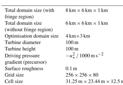
Table 1.Simulation parameters. Results remain dynamically equiv-alent for any selected value of the friction velocity u∗. The

hub-height velocity obtained in the precursor simulation corresponds to

u_h≈17.5u∗.

Total domain size (with 8 km×6 km×1 km fringe region)

Total domain size 6 km×6 km×1 km (without fringe region)

Optimisation domain size 4 km×3 km Turbine diameter 100 m Turbine height 100 m

Driving pressure −u2∗/1000 m s−2

gradient (precursor)

Surface roughness 0.1 m

Grid size 256×256×80

Cell size 31.25 m×23.44 m×12.5 m Time step 0.4/u∗s

In Fig. 2, a detailed convergence analysis of the farm power and the power output of a single turbine is shown for an aligned wind-farm layout (corresponding to Case 4 in Ta-ble 2 below). In Fig. 2a, a power histogram is shown for the wind farm, as well as for two individual turbines in the farm. Figure 2b shows results of the relative error P of the time average as a function of the averaging time T (see Eq. 1),

where

P(T)=

1

T

RT

0 P(t)dt−Pref

P_ref . (13)

For reference Pref we use an average obtained over a

pe-riod of 40/u∗h (withu∗=0.457 m s−1 taken as a realistic value, this corresponds to averaging over 88 h in physical time). It is seen from the figure that, for limited averaging times, errors can be quite significant, in particular when look-ing at the slook-ingle-turbine average. In fact, it is well known that the time average in turbulent flows converges asT−1/2

(see, e.g., Tennekes and Lumley, 1972). This is also seen in

Fig. 2b: errors decrease fast at low values ofT, but

after-wards convergence stagnates. This is particularly problem-atic when looking at the turbine average power, which re-quires roughly 15 to 20/u∗h to converge within 1 % of the reference average (requiring excessive computational costs – see below). It is further seen that the error on the over-all wind-farm power converges significantly faster, i.e. an error of 1 % is reached after approximately 5/u∗h. This is related to the fact thatNtpartly uncorrelated turbine power

signals are accumulated. Therefore, in order to limit com-putational effort related to LES in a hybrid Jensen–LES ap-proach, we will formulate our approach based on matching LES and Jensen farm power levels. In order to avoid overfit-ting of the Jensen wake-expansion coefficient, we use an en-semble of different wind-farm layouts that gradually evolve during optimisation towards layouts that are more optimal in terms of power extraction. This approach is further discussed in Sect. 2.4.

In terms of computational cost, the spin-up of the pre-cursor simulation is the most expensive (but needs to be done only once), amounting to 32 h of wall-clock time on the ThinKing cluster of the Flemish Supercomputer Cen-tre, using eight Ivy Bridge nodes consisting of two 10-core “Ivy Bridge” Xeon E5-2680v2 CPUs (2.8 GHz, 25 MB level 3 cache) for a total of 160 cores. Wind-farm spin-up takes around 14 h of wall-clock time on the same processor layout. Subsequent averaging takes around 9 h of wall-clock time per 3600/u∗s of wind-farm time. In order to keep overall computational costs under control, we limit time averaging in the current work to 3600/u∗s (roughly corresponding to at least 9u∗flow-through times). This yields an expected er-ror level on the power output of 2 % (see discussion above and Fig. 2b). In practice, for optimisation over a single at-mospheric conditionµ(e.g. a single wind direction), it may

be advisable to use at least 5/u∗h for the current case set-up. However, when considering optimisation over a range of conditions, the impact of this variability will be further aver-aged out.

(6)

Algorithm 2:The outline of the cross–entropy optimisation method for finding the optimum wind-farm layout. Values used in the current study areNiters= 2000,Ns= 1000,M= 200.

Input:Value of the wake expansion parameterkw, domainΩ, minimum distancedmin.

Output:An optimum wind-farm layout that generates maximum amount of energy. 1 fork←1toNiters

2 GenerateNsrandom layouts, where each random sample consists of a set coordinatesxi(i= 1···Nt). Samples are uniformly

distributed with mean value ofmk−1and deviation ofdk−1. Initial mean and deviation values are set to span the whole domain

Ω; 3 ifk >1then

4 Replace the first sample withSOPT;

5 forj←1toNs

6 Calculate the total power of layoutj(omithijin energy function fork≤M). 7 Sort theNssamples based on their total generated power in descending order. 8 Choose the bestNbsamples (we useNb= 0.4Ns).

9 Setmk_b−1anddk_b−1to be the mean and deviation of the bestNbsamples. 10 Calculatemkanddkusing (17,18).

11 Set the best sample as the optimum layoutSOPT.

cheap. In fact, as further discussed below, the main cost in our overall hybrid method remains associated with performing the LES.

3 Results

In the current section, optimisation results are discussed. First of all, in §3.1, the initial LES database for calibration of the Jensen model is constructed. Next, optimisation results of the Jensen only model are discussed in §3.2. Subsequently, hybrid

5

Jensen–LES optimisation results are presented in §3.3. Finally, optimisation for multiple wind directions is discussed in §3.4.

3.1 Set-up of LES database for initial calibration

A first step in Algorithm 1 is the generation of a LES database that is a starting point for the calibration of the Jensen model. Here we choose a mix of staggered, aligned layouts, and randomly generated layouts. An overview of the different cases, and their generated power is provided in Table 2. We normalize all results with the power output of a ‘wakeless’ wind-farm, i.e. a

10

wind-farm consisting of turbines that all have undisturbed inflow. In order to normalize all LES results in the same way, we use the averaged power output of turbines located in the first row of the aligned and staggered layouts and multiply it byNt(= 30) to find the ‘wakeless’ farm output. We then state every farm power output as a percentage of this ‘wakeless’

wind-12

Figure 2.Convergence analysis of wind-farm and turbine power of an aligned wind-farm case (Case 4 in Table 2).(a)Probability density function of wind-farm power output and power output of a front-row and back-row turbine.(b)Convergence error P as a function of averaging timeT for the wind-farm power, and for the power of a front-row and back-row turbine. Blue line: wind-farm power; green line:

first-row turbine; red line: last-row turbine.

2.4 Hybrid Jensen–LES approach and cross-entropy optimisation

In the current manuscript, we propose a hybrid Jensen–LES approach for wind-farm layout optimisation. To that end, the layout optimisation is based on the Jensen model, but the wake-expansion coefficient kw is iteratively used to fit the

Jensen model to a set of LES data that is gradually adapted to the layouts that are explored during optimisation. The ap-proach is summarised in Algorithm 2. Here, we describe the approach considering a single atmospheric condition µ

(see Eq. 2), e.g., a single wind direction. Generalisation is straightforward, and optimisation over different wind direc-tions will be discussed in Sect. 3.4.

In a first step, a set ofNLLES cases of regular and

ran-dom layouts are generated. This set is used to fitkw using

Algorithm 4 (see below). Subsequently, layout optimisation is performed using the Jensen model and Algorithm 3 (see further below). The optimal layout is then added to the set of LES cases, and a number ofN_R−1 (N_R < N_L) additional

random layouts are added as well. Moreover, theN_R LES

cases with lowest generated powers are removed from the set. This new set is used to refitk_w, subsequently starting a

(7)

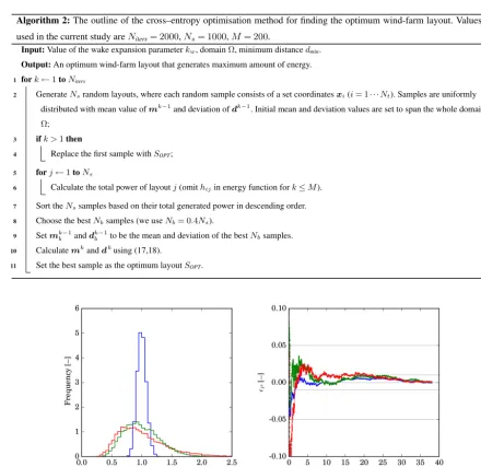
Algorithm 3:The outline of the cross–entropy optimisation method for optimising the wake expansion coefficient in the Jensen model using the LES data. Values used in the current study areNiters= 50,N= 1000.

Input:Total power ofNLwind-farm layouts obtained from LES simulations, each havingNtwind-turbines.

Output:An optimum value forkwthat minimises the error between predicted LES wind-farm power and Jensen wind-farm power. 1 Set the initial mean valuem(0)_{and deviation}_s(0)_;

2 fori←1toNiters

3 GenerateNrandom scalar samples, with uniform distribution with mean value ofm(i−1)_{and deviation of}_s(i−1)_;

4 ifi >1then

5 Replace the first sample withkw,OPT;

6 forj←1toN

7 Using samplejaskwin the Jensen model, calculate the relative wind-farm power ofNLlayouts.

8 Defineejas the sum of absolute value of errors between the Jensen model and LES wind-farm powers for theNLlayouts. 9 Sort theNsamples based on their error valueejforj∈ {1,···, N}, in ascending order.

10 Choose the first (best)Nbsamples (we normally setNb= 0.4N). 11 Setm(i)_and_s(i)_{to be the mean and deviation of the best}_N

bsamples. 12 Set the best sample as the optimum valuekw,OPT.

Table 2.Large Eddy Simulation results for different wind-farm layouts. Power output normalized with respect to total power of a wind-farm consisting of ‘first-row’ turbines. Average LES power is69.97%.

Case No. Description Relative wind-farm Power

1 Aligned with5D×5DSpacing 51.81%

5 Staggered with8D×5DSpacing 83.60%

6 Gradually staggered with8DSpacing 87.40%

7 Randomly generated withdmin= 2D 79.28%

farm output. Looking at the results of Table 2 it is apparent that the aligned cases perform quite poor in terms of relative power output, considerably worse than the staggered cases, but also worse than any of the random layouts that we investigated.

13

The procedure described above directly uses wind-farm power to fit the wake-expansion coefficient and avoids using errors on individual turbine power output. As discussed in Sect. 2.3, this reduces the need for time averaging in the LES, and significantly lowers computational costs. Moreover, by includingNLdifferent layouts, potential overfitting ofkwis

avoided, and the influence of remaining LES convergence er-rors on the optimal fit is further reduced.

For the layout optimisation in Algorithm 3 and the opti-mal fit ofk_w in Algorithm 4, we employ the cross-entropy

(CE) method. This method was originally developed to es-timate the probability of rare events. Later on, it was re-alised that it is also very effective in solving difficult non-convex optimisation problems. The method is explained in detail by De Boer et al. (2005) and Rubinstein (1999), among others. Here, we briefly review the main features of the ap-proach, as well as further detailing how we use it in a hybrid Jensen–LES optimisation of wind-farm layout. In our hybrid Jensen–LES optimisation approach of wind-farm layout, we use the CE method both for Jensen-based layout optimisa-tion, as well as for the adaptive fitting of the Jensen wake-expansion coefficient against a range of LES results (as fur-ther detailed below). However, it is important to emphasise that any feasible optimisation method may be used for this. For instance, recently, some work has focussed on the use of a gradient-based layout optimisation approach in combi-nation with engineering wake models (Fleming et al., 2016), while others have previously looked into the use of, for exam-ple, a particle-swarm method (Wan et al., 2010) and genetic algorithms (Chen et al., 2013a).

First of all, the optimisation problem Eq. (2) is slightly re-formulated in order to better cope with the second inequality constraint (as further discussed below, the first constraint is more straightforward to enforce directly). Therefore, we

con-sider following a non-smooth problem,

max

xi

Nt X

i=1

Pi(xi)+ Nt X

i=1

i−1 X

j=1

hij(xi,xj) (14)

subject to

xi∈, ∀i∈ {1,· · ·, Nt}, (15)

where

hij(xi,xj)=

−∞ kxi−xjk2< dmin

0 otherwise. (16)

This formulation is fully equivalent to Eq. (2).

The CE method for solving the optimal placement problem now essentially involves three steps. In a first step, a set of

N_suniformly distributed random samples of the optimisation

parametersxi are generated with a given mean value m(0) and deviationd(0) (note that bothmandd have dimension

2×Nt). At startup (iteration 0), no prior knowledge of the

optimisation problem is available, so we chose the mean and deviation such that the distribution spans the whole feasible parameter range. In the second step, samples are sorted

according to their energy function value. The bestNb< Ns samples are chosen, and the meanm(_bk)and deviationd(_bk)of

this set (in iteration stepk) is calculated. In a third step, a next

generation of samples (iteration stepk+1) is then created using a uniform distribution with a mean and deviation of

m(k+1)=m(k)+α(m(_bk)−m(k)), (17)

d(k+1)=d(k)+α(d(_bk)−d(k)), (18)

where the parameterαis selected in the[0,1]range, speci-fying how conservative or exploratory the algorithm is. This procedure continues until the end condition is met, which is

(8)

usually set by specifying the maximum number of iterations. We also transfer the optimum value in each generation to the next generation, so that the energy function value of the op-timum in each generation increases monotonically.

The treatment of the constraintxi∈is straightforward. Whenever a turbine location in a sample falls outside, the

location is simply orthogonally projected on the boundary of

. Note that turbines in samples in the initial generation

al-ways fall in, but in later generations, this is not always the

case. Though the projection on will slightly change the

distribution, as relatively more sample points can end up on the boundary, we did not find this to hamper the convergence of our algorithm. Finally, the treatment of the distance con-straint is implicitly handled by the energy function formula-tion and does not, in principle, require any further attenformula-tion.

Given the Jensen model, and an input for the wake-expansion coefficientkw, the cross-entropy layout

optimisa-tion is summarised in Algorithm 2, and specific choices are documented. We run the cross-entropy optimisation scheme forN_iter=2000 iterations; however, we find it beneficial for convergence and computational efficiency to omithij in the energy function during the firstMiterations, and to only

en-force thehij constraint fork > M. We takeM=200 in our implementation.

The standard deviation of samples in the cross entropy scheme eventually converge to zero. Once the standard de-viation has become small, and if the algorithm is locked in a local optimum, it will no longer break away from it. To re-duce the chance of this happening, we reset the calculated value ofdafter 1000 iterations. For turbines withx

coordi-nate less than 0.5 km or bigger than 3.5 km, we reset their

corresponding deviation to[0.5,0.5], and for the rest we re-set the deviation to[Lx/2, Ly/2]. This can be interpreted as running the cross entropy in two stages. Both run for 1000 iterations: the first runs starting with a uniform distribution in, and the second starts with the optimum layout of the

first stage as the mean value for its initial population. In the interest of simplicity, this detail is not included in the outline of Algorithm 2.

A second algorithm that is used in Algorithm 1 is the fit-ting of the wake-expansion coefficient k_w to the LES data.

Fitting k_w is also a non-convex optimisation problem, and

therefore we simply use the CE method again, but now for a scalar field. This is summarised in Algorithm 3. For this fit-ting, we found a number of iterations,Niters, of 50 sufficient

for good convergence.

We remark here that Algorithm 3 can in principle be used to fit more complicated relations forkw. For instance,

intro-ducing the heuristic dependencek_w=a+bx(or similar

ex-pressions), and fittinga andbinstead of the mean value of k_w, may be an interesting approach to represent the

down-stream development of k_w in the wind farm related to

in-creased turbulence levels. In the current work, we did not further explore this type of parameterisations ofk_w, as a

sim-105.7 103.2 97.4 99.4 94.3 52.6 51.2 51.6 51.3 49.2 58.2 54.8 55.0 57.2 54.9 58.6 55.7 56.1 58.3 55.1 59.3 56.7 56.7 58.2 53.2 58.1 56.3 59.5 59.3 54.2 95.2 91.6 96.1 100.9 91.1 106.3 101.4 94.6 93.7 95.1 74.7 74.1 72.9 75.5 72.3 75.5 72.7 73.7 72.6 73.3 74.9 72.9 70.2 71.8 69.1 75.3 69.2 72.5 68.7 71.3 90.0 79.5 36.2 101.5 91.8 66.1 54.1 99.2 49.3 53.7 89.7 72.0 82.0 92.7 45.1 95.3 80.0 55.4 107.4 96.6 93.1 77.8 55.6 49.8 94.2 91.5 81.5 80.6 59.4 57.1 75.8 58.6 64.4 89.4 81.7 97.3 79.2 59.6 38.2 66.2 89.6 104.1 96.8 93.8 84.2 100.8 94.3 83.9 58.7 80.0 62.8 92.7 71.2 92.0 38.2 94.6 68.0 96.7 67.1 100.9

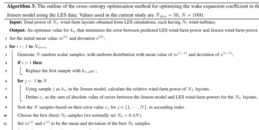
Figure 3.Layout and relative turbine power output for four of the cases listed in Table 2. Relative power results are obtained from large-eddy simulations. Turbine locations are marked with coloured disk: size and colour scale by relative power. Plot boundary (red line) corresponds to boundaries of domain(see Fig. 1).

ple fit of the mean value already leads to very satisfactory results (see next section).

Finally, we remark that the CE method is a global opti-misation method. However, its convergence to the global op-timum in a finite number of iterations can only be formally proven for some specific conditions; in practice, convergence depends on a number heuristic choices and is difficult to for-mally prove (see, e.g., Rubinstein and Kroese, 2013, for de-tails). In fact, this is a disadvantage that all global optimisa-tion methods share. However, the main advantage of using a global method is the fact that the algorithm does not get trapped in local optimums that easily. Moreover, the disad-vantage of the high number of function evaluations required for such global methods to work well is not really an issue, as Jensen-model evaluations are extremely cheap. In fact, as further discussed below, the main cost in our overall hybrid method remains associated with performing the LES.

3 Results

In the current section, optimisation results are discussed. First of all, in Sect. 3.1, the initial LES database for calibra-tion of the Jensen model is constructed. Next, optimisacalibra-tion results of the Jensen only model are discussed in Sect. 3.2. Subsequently, hybrid Jensen–LES optimisation results are presented in Sect. 3.3. Finally, optimisation for multiple wind directions is discussed in Sect. 3.4.

3.1 Set-up of LES database for initial calibration

(9)

“wake-Table 2.Large-eddy simulation results for different wind-farm layouts. Power output normalised with respect to total power of a wind-farm consisting of “first-row” turbines. Average LES power is 69.97 %.

Case no. Description Relative wind-farm power

1 Aligned with 5D×5Dspacing 51.81 %

5 Staggered with 8D×5Dspacing 83.60 %

6 Gradually staggered with 8Dspacing 87.40 %

7 Randomly generated withd_min=2D 79.28 %

less” wind farm, i.e. a wind farm consisting of turbines that all have undisturbed inflow. In order to normalise all LES re-sults in the same way, we use the averaged power output of turbines located in the first row of the aligned and staggered layouts and multiply it byN_t(=30) to find the “wakeless” wind-farm output. We then state every wind-farm power out-put as a percentage of this “wakeless” wind-farm outout-put. When looking at the results of Table 2 it is apparent that the aligned cases perform quite poorly in terms of relative power output and considerably worse than the staggered cases, but they also perform worse than any of the random layouts that we investigated.

In Fig. 3 the layout and relative power output of individ-ual turbines are shown for an aligned and a staggered lay-out as well as for two of the random laylay-outs. Wind direc-tion is always from left to right. First of all, we remark that there is still considerable variability at turbine level that is due to the limited averaging period of 3600/u∗s. As shown in Fig. 2b, variability in the turbine power average is in the order of±5 % or more, and this is in line with the variability observed in the first row of Fig. 3. We verified that first-row turbine averages all converge to a relative power of 100 % when averages of up to 15/u∗h are used. Finally, we note that the accumulated farm power is much better converged.

3.2 Comparison of Jensen model and LES results

Without access to reference results that can serve to tunek_w

in the Jensen model, it is possible to resort to Eq. (4) to deter-minek_w. Using this equation for our simulation set-up leads

to

kw= 0.41

ln(100/0.1) =0.060.

Here we briefly compare the Jensen model using this value with LES results. To do so, we use the 10 layouts presented in Table 2.

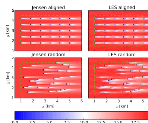
A comparison of flow fields as generated by the Jensen model and LES is shown in Fig. 4. It is seen that the

aver-Figure 4.Comparison of Jensen model and LES for an aligned and random layout.

aged flow data of LES are much smoother as a result of tur-bulent mixing. In contrast, in the Jensen model, wakes have a sharp boundary, also leading to sharply marked overlap re-gions. Note that mirror wakes also occur more downstream in the farm. Some features are not represented at all by the Jensen model. For instance, in the random layout, it is seen that side-by-side wakes can influence each other. Such be-haviour is not parameterised in the Jensen model.

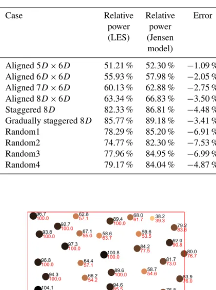
However, the most relevant property from a power optimi-sation point of view is the total error in the predicted power. In Table 3, the average power output from LES and the Jensen model is compared. It is seen that the Jensen model using k_w=0.060 is very accurate for some cases, but not

so for others. In particular, the cases that have a higher rel-ative power extraction are generally predicted worse by the Jensen model, than the cases with a lower relative power (the most prominent exception is Case 6). Another trend is that

(10)

Table 3. Comparing outputs of LES and the Jensen wake model withkw=0.060.

Case Relative Relative Error

power power (LES) (Jensen

model)

Aligned 5D×6D 51.21 % 52.30 % −1.09 % Aligned 6D×6D 55.93 % 57.98 % −2.05 % Aligned 7D×6D 60.13 % 62.88 % −2.75 % Aligned 8D×6D 63.34 % 66.83 % −3.50 % Staggered 8D 82.33 % 86.81 % −4.48 % Gradually staggered 8D 85.77 % 89.18 % −3.41 % Random1 78.29 % 85.20 % −6.91 % Random2 74.77 % 82.30 % −7.53 % Random3 77.96 % 84.95 % −6.99 % Random4 79.17 % 84.04 % −4.87 %

84.5 63.7

57.1 100.0

73.0 100.0

83.6 53.5

36.4

54.2 100.0

100.0 100.0 100.0

77.5 100.0

100.0 54.6 _76.0

76.7 57.1

100.0

53.9

90.8 39.3

85.5 61.7 100.0

55.0

100.0

75.8 58.6

64.4 89.4

81.7 97.3

79.2 59.6

38.2 66.2 89.6

104.1 96.8

93.8

84.2 100.8

94.3 58.7 _83.9

80.0 62.8

92.7

71.2

92.0 38.2

94.6 68.0 96.7

67.1

100.9

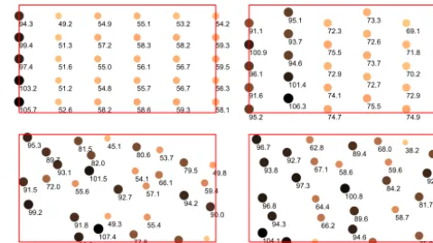
Figure 5.Comparing the wind-turbine power generation obtained from LES data (black numbers) and Jensen model (red numbers). Turbine locations are marked with coloured disk: size and colour scale by relative power. Plot boundary (red box) corresponds to boundaries of domain(see Fig. 1).

the regular cases are better predicted than the irregular cases. However, in the context of optimisation, it is not important for the Jensen model to be accurate over a wide range of dif-ferent layouts. Far away from the optimal layout, the required accuracy can be allowed to be considerably lower than close to the optimum. In this sense, Algorithm 2 gradually adapts the Jensen model through its wake-expansion coefficient to better fit more performing layouts.

Finally, when looking at turbine level in Fig. 5 for one of the random layouts (i.e. Case 10), it is seen that errors at the turbine level are much larger than the error on the accumu-lated power reported in Table 3. Again, from an optimisation point of view, this is less of an issue as long as a coupled ap-proach in combination with LES is used to adapt the model and verify the overall results close to the optimum. We fur-ther notice here that the statistical errors on the averaged tur-bine power output from LES are still significant due to the limited time of averaging (in the order of 5 % – see discus-sion in Sect. 3.1).

96.3 70.3_69.8

100.8 98.0

80.1

67.6 87.1

69.0

83.4 94.6

72.9 96.1

87.8

80.2 91.1

95.7

76.4 74.8

78.4 99.3

105.6

76.7

85.2

66.6 91.9

71.4

94.4 91.9

89.0

Figure 6.Optimal layout and relative power for a single wind direc-tion obtained after iteradirec-tion 1. Relative power results are obtained from large-eddy simulations. Turbine locations are marked with coloured disk: size and colour scale by relative power. Plot bound-ary (red line) corresponds to boundaries of domain(see Fig. 1).

79.2

100.3 71.7_82.4 84.1 94.6

71.3

100.1 93.6

97.7 98.5

102.1 93.9

90.9 96.2

76.4 74.9

83.5

98.8 91.8

73.8 78.9

83.6 95.1

85.5

86.4 95.6

80.0 71.4 98.7

Figure 7.Optimal layout and relative power for a single wind direc-tion obtained after iteradirec-tion 2. Relative power results are obtained from large-eddy simulations. Turbine locations are marked with coloured disk: size and colour scale by relative power. Plot bound-ary (red line) corresponds to boundaries of domain(see Fig. 1).

3.3 Hybrid Jensen–LES optimisation

Using Algorithm 2, we now optimise the wind-farm lay-out with a single constant wind direction given the set-up in Fig. 1 and wind coming from the left. Strictly speaking, this corresponds to the situation wheref_p(µ) in Eq. (2)

cor-responds to a Dirac delta function centred around an eastern wind direction, so that the integral over atmospheric condi-tions in Eq. (2) drops out. Optimisation over different wind directions is briefly discussed in Sect. 3.4. For the single wind-direction case considered here, only three outer itera-tions are required in the algorithm to converge to an optimal layout and optimally tuned Jensen model. Intermediate re-sults of these iterations are discussed below.

In iteration 1, we start Algorithm 2 with the initial cases shown in Table 2. Using these 10 cases, we use Algorithm 4 to optimise the value ofkw, finding a value ofkw=0.055.

Subsequently, this value is used to optimise the layout using Algorithm 3. The resulting optimal layout is shown in Fig. 6. Table 4 summarises the relative LES and Jensen power, as well as errors for the 10 initial training cases and for the newly obtained optimal layout. The relative power generated by the newly found optimum corresponds to 90.5 %

(11)

Table 4.Iteration 1: comparing outputs of LES and Jensen wake model withkw=0.055.

model)

Aligned 5D×6D 51.21 % 49.59 % 1.62 %

Aligned 6D×6D 55.93 % 55.40 % 0.53 %

Aligned 7D×6D 60.13 % 60.17 % −0.04 % Aligned 8D×6D 63.34 % 64.22 % −0.88 % Staggered 8D 82.33 % 85.78 % −3.46 % Gradually staggered 8D 85.77 % 92.27 % −6.50 % Random1 78.29 % 84.52 % −6.23 % Random2 74.77 % 81.23 % −6.46 % Random3 77.96 % 84.51 % −6.55 % Random4 79.17 % 83.27 % −4.10 % Optimum iter. 1 90.51 % 93.13 % −2.62 %

Table 5.Iteration 2: comparing outputs of LES and Jensen wake model withk_w=0.036.

model)

Staggered 8D 82.33 % 79.01 % 3.32 %

Gradually staggered 8D 85.77 % 93.06 % −7.29 % Random1 78.29 % 81.81 % −3.52 % Random3 77.96 % 82.27 % −4.31 %

Random4 79.17 % 77.80 % 1.37 %

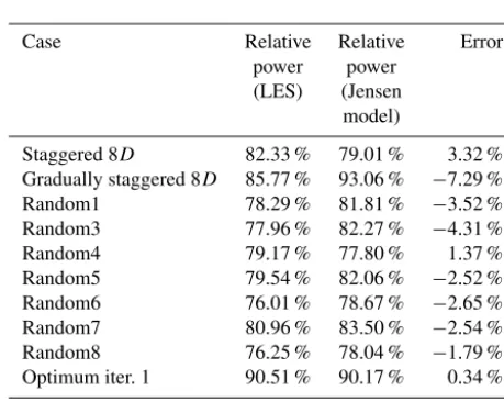
Random5 79.54 % 82.06 % −2.52 % Random6 76.01 % 78.67 % −2.65 % Random7 80.96 % 83.50 % −2.54 % Random8 76.25 % 78.04 % −1.79 % Optimum iter. 1 90.51 % 90.17 % 0.34 % Optimum iter. 2 92.04 % 91.88 % 0.17 %

In iteration 2, we add optimal layout 1 and four additional random layouts to the LES database and remove the 5 layouts with lowest relative power. Using Algorithm 4, we find a new valuekw=0.036 that best fits the Jensen model to the LES

data. Subsequently, using Algorithm 3, a new optimal layout is found, which is shown in Fig. 7. Furthermore, an overview of relative powers from LES and Jensen is shown in Table 5. It is seen that the new optimal layout leads to a relative power of 92.8% (evaluated using LES), but in contrast to the first it-eration, the error with the Jensen model remains now limited to 0.17 %.

As can be seen, the two optimum layouts, although ob-tained using different values of k_w, have the same general

structure.

Table 6.Optimum values ofk_wobtained in different iterations of

Algorithm 2.

Iteration optimum Relative LES

no. kw power of

corresponding optimum

layout

1 0.055 % 90.51 %

2 0.036 % 92.04 %

3 0.036 % NA

NA: not available.

In iteration 3, we repeat the procedure a third time and find (almost) the same value forkw. Only the fourth digit differs,

and the resulting new optimal layout remains the same. In fact, we observed that up to changes in the second digit, the value ofk_wdoes not significantly influence the optimal

lay-out. Finally, the error between the Jensen model and the LES is below 1 %, which corresponds roughly to the statistical av-eraging accuracy of the LES. We conclude that the algorithm is converged.

After initial set-up of the LES database, each main opti-misation step requires 2.5×106Jensen evaluations per itera-tion and five LES evaluaitera-tions. Wall time for the Jensen eval-uations (per iteration) corresponds roughly to 1.25 h on one

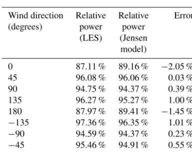
Ivy Bridge node of the ThinKing cluster of the Flemish Su-percomputer Centre. Total wall time for LES (per iteration, and excluding the precursor spin-up time – see Sect. 2.3) amounts to approximately 70 h on eight nodes of the Flemish Supercomputer, equivalent to 560 node hours. Even though the Jensen model is 500 000 times more evaluated per itera-tion than LES, the total LES cost is roughly 500 times more expensive and the LES wall time is roughly 50 times longer. Given this single wind direction, the optimal layout leads to a relative wind-farm performance of around 93 % of a wakeless wind farm, which is considerably higher than a typ-ical aligned or staggered layout. Moreover, when looking at the layout that was found in Fig. 7, it is observed that turbines are grouped into two main clusters – one at the front of the farm and one at the back of the farm, leaving a large stream-wise distance in between for wake recovery. Obviously, this result is particular for a single wind direction. In the next section, we study the cases with multiple wind directions.

Finally, we remark that it is difficult to prove formal con-vergence of the CE method that we use for our optimisation (see discussion at the end of Sect. 2.4), and optimisation is terminated based on a maximum number of iterations in Al-gorithms 2 and 3. Therefore, we checked the dependence of our results versus the initial starting point of the optimisa-tion. We found that a change in initial distribution leads to slight shifts in the turbine locations, but this does not sig-nificantly influence the value of the power extraction.