The Influence of Grid Orthogonality on the Convergence of the SIMPLE Algorithm for Solving Navier-Stokes Equations

Strojniški vestnik - Journal of Mechanical Engineering 53(2007)2, 105-113 UDK - UDC 519.65:004.021

Kratki znanstveni prispevek - Short scientific paper (1.03)

Vpliv pravokotnosti mreže na konvergenco programa SIMPLE

za reševanje Navier-Stokes-ovih enačb

The Influence of Grid Orthogonality on the Convergence of the SIMPLE Algorithm

for Solving Navier-Stokes Equations

Ivo Džijan - Zdravko Virag - Hrvoje Kozmar (University o f Zagreb, Croatia)

Razvili smo metodo končnih volumnov za reševanje Navier-Stokesovih enačb na lokalno pravokotni nestrukturirani mreži z uporabo algoritma SIMPLE. Razvito metodo smo primerjali s podobno metodo na strukturirani, ne nujno pravokotni mreži, v členih pretekle konvergence in obsegu pod-relaksacijskih faktorjev, p ri katerih se metodi približujeta. Kadar j e strukturirana mreža pravokotna, sta stopnji približevanja obeh metod podobni. Vprimerih, kadar strukturirana mreža ni pravokotna, se pokaže prednost predlagane metode pri lokalno pravokotni mreži v razmerah pretekle konvergence. V teh primerih je obseg pod-relaksacijskih faktorjev, pri katerih je predlagana metoda zadovoljivo konvergentna, mnogo večji kot pri metodi na nepravokotni mreži.

© 2007 Strojniški vestnik. Vse pravice pridržane.

(Ključne besede: Navier-Stokesove enačbe, metode končnih volumnov, algoritmi SIMPLE, nestrukturirane mreže)

A finite-volume method fo r solving the Navier-Stokes equations on a locally orthogonal unstruc­ tured grid using the SIMPLE algorithm has been developed. The developed method was compared with a similar method on a structured, not necessarily orthogonal grid, in terms o f convergence history and the range o f under-relaxation factors in which the methods converge. When the structured grid is orthogonal, the convergence rates o f the two methods are similar. For the cases when the structured grid is non-orthogonal, the superiority o f the proposed method on the locally orthogonal grid is demonstrated in terms o f convergence history. In these cases, the range o f under-relaxation factors in which the proposed method shows satisfactory convergence is much wider than fo r the method on the non-orthogonal grid.

© 2007 Journal o f Mechanical Engineering. All rights reserved.

(Keywords: Navier-Stokes equations, finite volume methods, SIMPLE algorithm, unstructured grid)

0 INTRODUCTION

The rapid developm ent o f computers has brought about rapid developments in the field of computational fluid dynamics. Calculation domains are now more complex, which increases the need to use an unstructured grid for their discretization. Finite volume methods are widely applied for solving fluid flow problems. Initially, these methods were used on structured staggered grids. Nowadays they are used on unstructured collocated grids, on which segregate algorithms with the pressure-based ap­ proach are applied for incompressible flows. The most popular algorithm based on pressure correction is the SIMPLE (Semi-Implicit Method for the

Pressure-Linked Equation) algorithm, Caretto et al. [1] and Patankar and Spalding [2], In the pressure-velocity correction relation the effécts coming from velocity corrections in neighboring nodes on the pressure correction in the central node are neglected. The consequence o f this neglecting is the overestima­ tion p f the pressure correction, which can cause the divergence o f the numerical process. To ensure the stability o f the numerical process, the under-relax­ ation factor for the pressure is introduced. The opti­ mal value o f this factor cannot be estimated in ad­ vance since it depends on the grid’s characteristics and the nature o f the problem.

in the cell centre and the velocity components are calculated on the cell faces. On a collocated grid, the pressure field and velocity components are calcu­ lated in the cell centre. The application o f the SIMPLE algorithm on a collocated grid started with Rhie and Chow [3],

The grid non-orthogonality is one o f the fac­ tors that increases the number o f iterations o f the SIMPLE algorithm. If the connecting line o f two neighboring nodes is not perpendicular to the cell fa c e , som e te rm s th a t a p p e a r d ue to n o n ­ orthogonality are usually neglected. This is the case with the CAFFA public-domain computer code [4], It is believed that this neglecting slows down the rate o f convergence o f the n um erical m ethod. Therefore, the m odification o f the finite volume method on an unstructured locally orthogonal grid is proposed. The rate o f convergence o f the SIMPLE algorithm on that grid will be compared with the rate o f convergence on a structured, not necessarily orthogonal grid.

1 MATHEMATICAL MODEL AND NUMERICAL PROCEDURE

The mathematical model o f steady, laminar, incompressible fluid flow with constant viscosity and without mass forces is adopted. The model is d e s c rib e d w ith th e fo llo w in g N a v ie r-S to k e s equations:

_d_ dXj(■Pviv<)

dp d \

— + p--- —

dxt dxjdxj

(1)

(

2

Fig. 1. A part o f calculation domain and a typical cell o f locally-orthogonal unstructured grid

where p, v.,p, pandx. are the fluid density, velocity, pressure, viscosity and coordinates, respectively. These equations will be numerically solved on an unstructured locally orthogonal grid. A part o f such a computational grid is shown in Fig. 1.

The main nodes, C and N, at which the veloc­ ity and pressure fields are calculated, are placed within their respective cells. The connecting line CN is perpendicular to the cell face and the nodes C and N are at an equal distance from an auxiliary node n, which enables a simple formulation o f the high-order interpolation. It is clear that such a grid is possible in every 2D case, because the cell vertex a in Fig. 1 is the circumcenter o f the triangle formed by the nodes C, M and K. Such a grid generator is described by Džijan [5], which includes a grid-smoothing proce­ dure that forces the main nodes to be close to the cell centroids and the auxiliary nodes to be close to the cell-face centroids.

Discretization o f the equations starts with in­ tegrating over the cell volume V, according to Fig. 1. By using the Gauss theorem and the mean-value theorem, the integrated governing equations take the form:

± [ F f = 0 (3)

k=1

m

z

k=\

(4)

F v \ - p A = - V dp_

dx. pAdx.

where F = p A v n , = pAvn is the mass flow through the cell face and J t = F v f - pA (dvi / dx} ) is the momentum flux through the cell face. A ancf n are the cell-face area and its outward normal vector, F is the cell volume, while k denotes the cell-face index and

m is the num ber o f cell faces on the considered volume. The scope o f the differencing schemes is to define the velocity v,.| and its normal derivatives at the auxiliary node n in terms o f velocity values at the m ain nodes. Since the adopted grid is locally orthogonal, these values are defined by using only the values at nodes C and N. A blending scheme of the central differencing scheme (CDS) and o f the first-order upwind differencing scheme (UDS) is used in the CAFFA computer code. Therefore, the same scheme will also be used in the proposed method. In the case o f the locally orthogonal grid, the diffusion part o f the flux vector is m odeled w ith the following equation:

J f = - P A ^

In the case o f a non-orthogonal grid, an additional term appears. In the CAFFA computer code this term is implemented by using the deferred correction ap­ proach, i.e., by using the velocity values from the previous iteration.

In the first-order UDS, the convective flux is modelled by:

uns i fv -L f o r F>0 /z-s J UDS = F v | =<! ,c (6),

' “ [ Fv,.|n f o r F<0

and in the CDS (for the case when the node n lies in the middle o f the CN connection line) by:

(7).

By introducing the mixing factor y the final expression for the momentum flux is:

Ji = { i ~ r ) J - ' m + r j r + J t (

8

where, for y= 0 the result is the UDS, and for y= 1 the CDS.

Introducing the expressions for the fluxes into (4) results in:

ac vi lc - Ž [ aN v,- |N ]* = + b,

where:

m a x (-F ,0 ) + ^

2s.

(9)

(10),

(11)

and

bt = y É | V v.In1 -Ì;[max(-F,0)]‘v,|c + É[n>ax(-F,0)v,|N]‘}

* = i L z J *= i *=i

(

12

It is obvious that all the terms coming from the CDS are treated as a deferred correction, the same as in the CAFFA code.

To reduce the possibility that the numerical process diverges, this equation is under-relaxed in the following form:

u - L acV,|c - £ [ a Nvf|N] = - V ~ - +

b,+-(13) which was proposed by Patankar [6], The last term on the right-hand side is calculated from the previ­ ous iteration, and ₇ a is the under-relaxation factor

UV for the velocity.

According to Rhie and Chow [3], the mass flow through the cell face is defined as follows:

F = pAvn = pA(vn) - p A dp (dp

\

U n J dn□ ^dnn J

where the line above a symbol indicates the linear interpolation between the values at nodes C and N, as follows:

and

( v „ ) = — ( v , | + v . l i n , .

\ n j o V 7 l e -Mn/ j

(v.1

' dp

_V

_J

: I |

2 1dn & dn

( K ) 1 f K . i v H Ì

“ 2 l ( ß c ) |c ( O c ) |N J

(15) ,

(16)

(17).

In the case o f a locally orthogonal grid, the normal derivative o f the pressure is defined by using the CDS, as follows:

dP _ Fn Pc

dn n 2s (18).

In the CAFFA code, where the grid is non- orthogonal, additional terms emerge and are treated explicitly by using the values from the previous iteration.

Solving the momentum equation with a given pressure field p ‘ results in the velocity field v *, and the mass flow F*, which does not necessarily satisfy the continuity equation. For that reason, the velocity corrections y ’ and the corresponding F ’ and pres­ sure correction p ’ are searched, so that the corrected velocity field v. = v." + v ’ and corrected mass flow F = F* + F ’ satisfy the continuity equation. Accord­ ing to Equation (14), the corrected mass flow is ap­ proximated as follows:

F = F * - ^

2s (Pn-■Pc) ~a N ( Pn Pc)

(19).

Introducing the corrected mass flows in the continuity equation (3) results in the following equation for the pressure correction:

where

and

m ,

ac Pc - Z [ön’Pn] = b P

k= 1

< ' = Z K T

Jt=l

(20)

(

)

(

22

field is corrected using the following equation:

P c= P c+ a PPc (23) where a is the under-relaxation factor for the pressure. The velocities in the main nodes are corrected as follows:

V_ty_

a c dx,

(24).

The gradients o f the physical values in the main nodes are calculated using the Gauss formula as follows:

V 2V

m

Y X ^pA (25)

where <j) can stand for v ,p or p

The steps in the SIMPLE algorithm for solv­ ing the Navier-Stokes equations can be summarized as follows:

1. Guess the pressure fieldp* and the velocity field y . 2. Solve the momentum equation ( 13) to obtain y*. 3. Solve the p ’ equation (20). Correct the pressure

according to (23), correct the velocity according to (24) and the mass flow according to (19). 4. Treat the corrected pressure as p* and return to

Step 2. R epeat the w hole procedure until a converged solution is obtained.

The converged solution is obtained when the n o rm a liz e d re s id u a ls fo r th e c o n tin u ity and mom entum equations become smaller than some small number, s. In this paper s= 10‘6 was used. The residual for the continuity equation is:

(26)

and the residual for the momentum is

M

* V , = I

/=1 k= 1

i „ T + F & 1 $3-

___

1

InJ dx, _C (27).

In the above expressions, / denotes the cell index and M th e total number o f cells. The values o f the variables in the above form ula are from the current iteration, and the coefficients are prepared for the next iteration. The following residuals are usually normalized: the mass residuals w ith the inlet mass-flow rate and the residuals for the momentum equation with the inlet momentum flow rate.

2 RESULTS

The described numerical method is im ple­ mented in the FVM computer code. In this code the

residuals are defined and normalized in the same way as in the CAFFA code. The rate o f convergence o f the described method and o f the method used in the CAFFA code will be compared by varying the grid’s non-orthogonality and the differencing scheme. Also, the range o f under-relaxation factors in which the numerical procedure converges will be analyzed.

2.1 Laminar flow in a lid-driven cavity with inclined side walls

In this test the 2D laminar fluid flow is calcu­ lated in a closed cavity whose lid is moving in a tangential direction with velocity v Perič [7]. The R eynolds num ber based on the side length a is R e =p.y.atp= 1000. The calculation is performed for different inclination angles o f the side walls, ß= 90°, 67.5° and 45°. In this problem the residuals defined by (26) and (27) are not normalized.

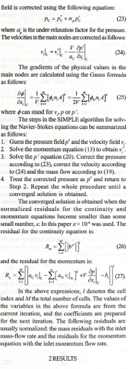
Fig. 2 shows the qualitative picture o f the streamlines for /7= 90° and 45°. It is obvious that the initially assumed constant-velocity field will be very different from the final solution.

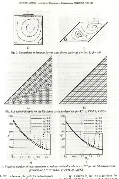
The problem is solved using the CAFFA nu­ merical code on structured grids o f size 40x40 cells, and with the FVM code on unstructured grids with approximately 1600 cells. Fig. 3 a shows a part o f the unstructured grid for ß= 45° that is used in the FVM code. The borders o f the finite volum es are pre­ sented, and the main nodes are marked. Fig. 3 b shows a part o f the geometric grid for the same case, which is used in the CAFFA code. The displayed lines connect the main nodes at which the pressure and velocity fields are calculated.

In the SIMPLE algorithm, two under-relaxation factors should be given. The rate o f convergence de­ pends on the values o f these two factors. Their optimal values are not known in advance, so that the described problem will be solved for a range o f under-relaxation factors by varying am from 0.5 to 0.95 with a step o f 0.025, and ap from 0.1 to 0.6 with a step o f 0.1. The comparison criteria will be the number o f iterations needed for the residuals to fall below s= 10"6.

In the CAFFA and FVM codes different sol­ vers for linear algebraic equations are used. For this reason, a sufficient number o f inner iterations is given at every iterative step to be sure that the systems are solved equally well in both codes.

Fig. 4 shows the numbers o f outer iterations

Fig. 2. Streamlines in laminar flow in a lid-driven cavity a) ß = 90°, b) ß = 45°

b)

Fig. 3. A part o f the grid fo r the lid-driven cavity problem fo r ß = 45° a) FVM, b) CAFFA

Fig. 4. Required number o f outer iterations to reduce residual levels to s = 1 O'6 fo r the lid-driven cavity problem fo r ß = 90° (UDS) a) FVM, b) CAFFA

for ß= 90°. In this case, the grids for both codes are orthogonal, and the achieved results are almost iden­ tical. This confirms the equivalent implementation o f the SIMPLE algorithm in both codes.

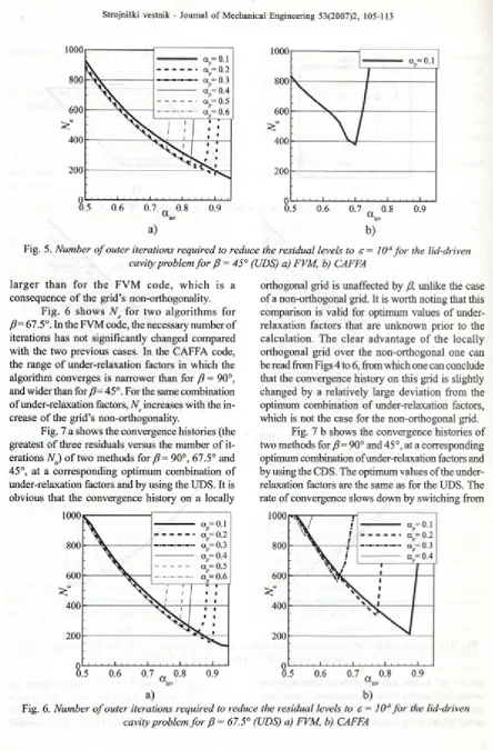
Fig. 5 shows N c for tw o algorithm s for

ß= 45°. The SIMPLE algorithm in the CAFFA code converges in that situation only in the case that

Fig. 5. Number o f outer iterations required to reduce the residual levels to e = 1 O'6 fo r the lid-driven cavity problem fo r ß = 45° (UDS) a) FVM, b) CAFFA

la rg e r th a n fo r th e F V M co d e, w h ic h is a consequence o f the grid’s non-orthogonality.

Fig. 6 show s N e fo r tw o alg o rith m s for /?= 67.5°. In the FVM code, the necessary number o f iterations has not significantly changed compared with the two previous cases. In the CAFFA code, the range o f under-relaxation factors in which the algorithm converges is narrower than for ß = 90°, and wider than for ß= 45°. For the same combination o f under-relaxation factors, N increases with the in- crease o f the grid’s non-orthogonality.

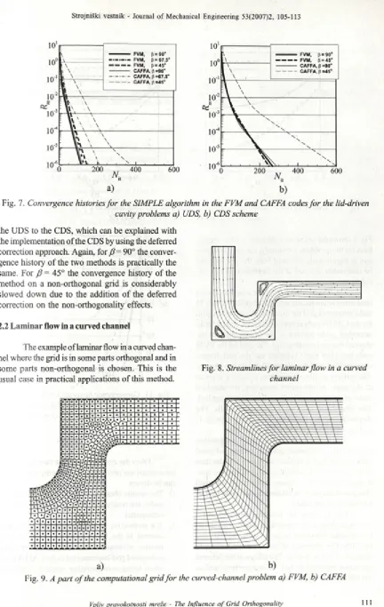
Fig. 7 a shows the convergence histories (the greatest o f three residuals versus the num ber o f it­ erations N .) o f two methods for ß = 90°, 67.5° and 45°, at a corresponding optimum combination o f under-relaxation factors and by using the UDS. It is obvious that the convergence history on a locally

orthogonal grid is unaffected by ß, unlike the case o f a non-orthogonal grid. It is worth noting that this comparison is valid for optimum values o f under­ relaxation factors that are unknow n prior to the calculation. The clear advantage o f the locally orthogonal grid over the non-orthogonal one can be read from Figs 4 to 6, from which one can conclude that the convergence history on this grid is slightly changed by a relatively large deviation from the optimum combination o f under-relaxation factors, which is not the case for the non-orthogonal grid.

Fig. 7 b shows the convergence histories o f two methods for ß= 90° and 45°, at a corresponding optimum combination o f under-relaxation factors and by using the CDS. The optimum values o f the under­ relaxation factors are the same as for the UDS. The rate o f convergence slows down by switching from

a) b)

a) b)

Fig. 7. Convergence histories fo r the SIMPLE algorithm in the FVM and CAFFA codes fo r the lid-driven cavity problems a) UDS, b) CDS scheme

the UDS to the CDS, which can be explained with the implementation o f the CDS by using the deferred correction approach. Again, for ß — 90° the conver­ gence history o f the two methods is practically the same. For ß = 45° the convergence history o f the m ethod on a non-orthogonal grid is considerably slowed down due to the addition o f the deferred correction on the non-orthogonality effects.

2.2 L am in ar flow in a curved channel

The example of laminar flow in a curved chan­ nel where the grid is in some parts orthogonal and in some parts non-orthogonal is chosen. This is the usual case in practical applications o f this method.

Fig. 8. Streamlines fo r laminar flow in a curved channel

a) b)

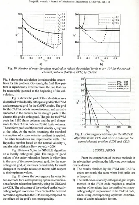
Fig. 10. Number o f outer iterations required to reduce the residual levels to s = 1 O'6 fo r the curved-channel problem (UDS) a) FVM, b) CAFFA

Fig. 8 shows the calculation domain and the stream­ lines for this problem. Obviously, the final flow pat­ tem is significantly different from the one that can be reasonably guessed at the beginning o f the cal­ culation.

Fig. 9 shows the part o f the calculation area discretized with a locally orthogonal grid for the FVM and a structured grid for the CAFFA codes. The grid for the CAFFA code is non-orthogonal, and partially smoothed in the comers. In the straight parts o f the channel this grid is orthogonal. The grid for the FVM code has 1180 finite volumes and the grid dimen­ sions for the CAFFA code are 20x60 finite volumes. The uniform profile o f the normal velocity vn is given at the inlet. A t the outlet boundary, the standard assumption o f a zero velocity gradient is applied. The other boundaries are impermeable walls. The Reynolds number based on the normal velocity vn and the inlet width a is Re = p v nalp = 200.

Fig. 10 shows Ne for the SIMPLE algorithm on a locally orthogonal grid. The range o f good values o f the under-relaxation factors is w ider than in the case o f the non-orthogonal grid. For the non- orthogonal grid, N£ increases considerably for small changes o f the under-relaxation factors w ith respect to their optimum values.

Fig. 11 shows the convergence histories for two methods for a corresponding optimum combina­ tion o f under-relaxation factors by using the UDS and the CDS. The advantage o f the method on the locally orthogonal grid is obvious. The effects o f the deferred correction approach in the CDS are superimposed on the effects o f the grid’s non-orthogonality.

Fig. 11. Convergence histories fo r the SIMPLE algorithm in the FVM and CAFFA codes fo r the

curved-channel problem (UDS and CDS)

3 CONCLUSIONS

From the comparison o f the two methods in the selected test problems, the following conclusions can be drawn:

1) The results obtained by the FVM and CAFFA codes are nearly the same when both grids are orthogonal.

3) The ran g e o f u n d e r-re la x atio n facto rs for w hich the m ethod converges is narrow ing w ith th e in c r e a s e o f th e g r i d ’s n o n ­ orthogonality. This is a serious draw back, if we know that the optim um values o f the un­ der-relaxation factors are not know n in ad­

vance, and that they take different values from problem to problem.

4) The application o f the CDS based on the de­ ferred correction approach increases the required number of iterations. This effect is superimposed on the effects o f the grid’s non-orthogonality.

4 LITERATURE

[1] Caretto, L.S., A.D. Gosman, S.V. PatankarundD.B. Spalding (1972) Two calculation procedures for steady, three-dimensional flows with recirculation. Proceedings o f Third International Conference on Numerical Methods in Fluid Dynamics, Paris.

[2] Patankar, S.V., D.B. Spalding (1972) A calculation procedure for heat, mass, and momentum transfer in three dimensional parabolic flows. Int. J. Heat Mass Transfer, 15(1972), pp. 1787-1806.

[3] Rhie, C.M., W.L. Chow (1983) A numerical study of the turbulent flow past an isolated airfoil with trailing edge separation. 21(1983), pp. 1525-1532.

[4] Ferzinger, J. H., M. Perič (1996) Computational methods for fluid dynamics. Springer-Verlag, New York. [5] Džijan, I. (2004) Numerical method for fluid flow analysis on unstructured grid (in Croatian), PhD. Thesis.

University o f Zagreb, Faculty o f Mechanical Engineering and Naval Architecture, Zagreb. [6] Patankar, S. V. ( 1980) Numerical heat transfer and fluid flow. McGraw-Hill, New York.

[7] Perič, M. (1990) Analysis o f pressure-velocity coupling on nonorthogonal grids. Numerical Heat Transfer,

PartB; 17(1990), pp 63-82.

Authors’ Addresses: Doc. Dr. Ivo Džijan Prof. Dr. Zdravko Virag Dr. Hrvoje Kozmar University o f Zagreb

Faculty o f Mechanical Engineering and Naval Architecture

I. Lučića 5

HR-10000 Zagreb, Croatia [email protected] [email protected] [email protected]

Prejeto:

Received: 6.4.2006

Sprejeto:

Accepted: 22.6.2006