JIEMS
Journal of Industrial Engineering and Management Studies
Vol. 6, No. 2, 2019, pp. 196-213
DOI: 10.22116/JIEMS.2019.94158
www.jiems.icms.ac.ir
A novel multi-objective model for two-echelon green routing
problem of perishable products with intermediate depots
Erfan Babaee Tirkolaee1,*, Shaghayegh Hadian1, Hêriş Golpîra2
Abstract
Multi-echelon distribution mechanism is common in supply chain design and logistics systems in which freight is delivered to the customers through intermediate depots (IDs), instead of using direct shipments. This primarily decreases the cost of the chain and consequences of environmental (energy consumption) and social (traffic, air pollution, etc.) logistic operations. This paper develops a novel multi-objective mixed-integer linear programming model (MOMILP) for a two-echelon green capacitated vehicle routing problem (2E-CVRP) in which environmental issues and time windows constraints are considered for perishable products delivery phase. To validate the proposed mathematical model, several numerical examples are generated randomly and solved using CPLEX solver of GAMS software. The ε-constraint method is applied to the model to deal with the multi-objectiveness of the proposed model. Finally, the best Pareto solution for each problem is determined based on the reference point approach (RPA) as one of the most effective techniques to help the decision-makers.
Keywords: Two-echelon green routing problem; Intermediate depots; ε-constraint method; Perishable product distribution; Reference point approach.
Received: July 2019-11
Revised: August 2019-31
Accepted: October 2019-19
1. Introduction
A supply chain is a network of facilities organized to acquire raw materials, convert them to finished products, and distribute the products to consumers. Organizational relationships and strategic alliances and partnerships are crucial for supply chain management success (Golpîra, 2016; Golpîra et al., 2017a). So, supply chain network coordination is a vital decision affecting the future success of the business (Khan et al. 2019a). In today’s competitive environment, minimizing the operational cost plays an important role for companies along the coordinated supply chains. Industrialization, on the other hand, makes pollutions a serious issue. Dealing with such contradiction, transportation should be more considered along the supply chain (Khan et al., 2019b). Hence, constructing optimal routes to
* Corresponding author; [email protected]
serve customers to minimize the total cost and emissions is of interest for academicians and practitioners. In this way, a classical vehicle routing problem (VRP) was introduced by Dantzig and Ramser (1959) to determine an optimal set of routes for a fleet of vehicles to serve a given number of the customers and minimize total traveled distance. Besides, each customer should be served by exactly one vehicle that starts its trip from a depot and ends in the depot. VRP problems considering vehicles’ capacity constraints are called Capacitated Vehicle Routing Problem (CVRP), which has been studied by many researchers in many industries (Mandziuk and Swiechowski, 2017). Managers have to make some limitations on heavy vehicles moving in urban areas. However, large vehicles are used for transferring cargos from the depot located on the outskirts of the cities to the Intermediate Depots (IDs). And, small vehicles are used to transfer cargos from IDs to the customers located in the metropolitan areas. So, forming a two-echelon distribution system has been proposed by Wang et al., (2017). Two-Echelon Capacitated Vehicle Routing Problem (2E-CVRP) is a well-known distribution system in which IDs are located between suppliers and customers (Gonzalez-Feliu et al., 2008). Direct shipments from suppliers to customers are not allowed in this system (Jabali et al., 2012; Kritikos and Ioannou, 2013). This transportation network consists of two-echelons. 1) The 1st echelonrouting including determining the optimal routes of vehicles, which start from the central depot (supplier) and end at the IDs. 2) The 2nd echelon routing as the determination of optimal routes, which start from IDs and ends at the customers’ nodes. In each echelon, a homogeneous vehicle fleet is used. It is because of the fact that by using optimization approaches, only a few designs need to be assessed, hence the necessary computational time to achieve an optimal design is dramatically decreased (Golpîra, 2019). 1st echelon vehicles are located in the central depot and only fulfill the IDs demands, whereas 2nd echelon vehicles have lower capacities and provide customers’ demands through IDs. The unloading of the 1st echelon vehicles and loading of the 2nd echelon vehicles at the IDs contain a proportion of operational costs to the quantity loaded/unloaded additional to the vehicles’ usage costs. The 2E-CVRP aims to find a set of routes in each echelon to minimize the total vehicles usage and routing cost considering the assumption that each customer can only be visited once (Perboli et al., 2011; Baldacci et al., 2017).
Recent growing attention to the environmental issues, on the other point of view, is an important perspective in transport systems (Khan et al., 2018, 2019c). In this way, reducing CO2 emissions is the best way in building an environmental-friendly society (Yu et al., 2018). And, different speeds of the vehicles, as well as the number of carrying loads, are directly related to the fuel consumption and CO2 emissions (Franceschetti et al., 2013; Soysal et al., 2015).
Crainic et al. (2012) examined total routing costs minimization of the overall two-echelon network in a 2E-CVRP. They considered more realistic assumptions in urban cargo delivery where the travel costs depend directly on the distances, fixed cost of arcs usage, operational costs, and environmental costs. However, they didn’t consider the diversity of the arcs’ travel cost over time periods in the planning horizon. Soysal et al. (2015) presented a Mixed Integer Linear Programming (MILP) model for a time-dependent 2E-CVRP considering different vehicle types, vehicle speed, load, and emissions as well as multiple time zones. They solved a small real-world instance by CPLEX to show the applicability of their model for economies of environmentally friendly vehicle routing.
mathematical model to maximize the total level of customer satisfaction, which depends on the freshness of deliverables, where each vehicle has a maximum allowable delivery time. Esmaili and Sahraeian (2017) presented a 2E-CVRP model with the aim of minimizing customers' waiting time and total travel cost considering environmental issues for perishable goods. They used a Single Additive Weighting (SAW) method to solve the problem. Tirkolaee et al. (2017) developed a novel model for the robust multi-trip vehicle routing problem with intermediate depots and time windows in order to determine the optimal routes in a single-echelon supply chain for perishable products. They solve the model using CPLEX solver and demonstrated the validity of their proposed model by generating and illustrating different problems. Developing an Integer Linear Programming (ILP), Marandi (2017) developed an approach for solving an integrated production-distribution scheduling problem for perishable products and solved it using a graph-based heuristic method. More recently, Shahparvari and Bodaghi (2018) proposed a MIP model to support tactical decision making in assigning and distribution of perishable rescue items. They solved a VRP using time windows (VRPTW) by CPLEX solver for multiple perishable products distribution using historical data related to a case study. A two-echelon Inventory-Routing Problem (IRP) for perishable items was investigated by Rohmer et al. (2019). They designed three metaheuristic algorithms to solve the problem and could compare the obtained results against CPLEX. Rahbari et al. (2019) proposed two robust bi-objective mathematical models for VRP with cross-docking for perishable products with the aims of cost minimization and freshness maximization. The Lp metric method was used to provide single-objective models. Finally, they implemented the model using CPLEX solver of GAMS software and performed comparative analyses. In terms of greenness consideration, Golpîra (2016) and Golpîra (2017b) introduced a new model to formulate a green supply chain network through a MILP formulation. Yavari and Zaker (2019) designed a resilient-green supply chain for perishable products considering environmental concerns. They formulated the problem using a bi-objective MILP model and could investigate a real case study in a dairy company. A heuristic approach was developed by Yavari and Geraeli (2019) for designing a green closed-loop supply chain network of perishable products. They implemented their proposed algorithm to solve a real case study problem considering multiple products and multiple periods.
Based on the aforementioned literature review, this paper would cover the research gaps by developing a novel bi-objective model for green 2E-CVRP with intermediate depots for delivering perishable products. Two types of time windows are considered to define the applicability of the perishable products in the proposed approaches. The first objective is defined to minimize total travel costs including routing costs, usage costs of the vehicles, loading/unloading operations costs, and earliness and tardiness penalties of IDs/customers deliveries in the 1st/2nd echelon, and the second objective is devoted to minimize the total CO2 emissions along the supply chain. Hence, a multi-objective MILP (MOMILP) model is developed to formulate the problem with regards to the real-world assumptions. Then, the exact ε-constraint method is applied to the model in order to deal with bi-objectiveness. Finally, reference point approach (RPA) is implemented as one of the best techniques to find the best Pareto solution.
2. Problem Definition
In this section, a bi-objective model is developed and explained for the green 2E-CVRP with intermediate depots of perishable product distribution in order to determine the optimal routes for the vehicles in each echelon concerning economics and environmental aspects. The main characteristics applicable to the problem are to consider hard and soft time windows representing the nature of perishable products distributions. Serving the customers out of soft time windows may cause some penalty cost, but it is impossible out of hard time window. Serving out of hard time windows would lead to perished products.
Figure 1 shows this two-echelon planning for the proposed supply chain design. In this example, 1 central depot (supplier), three IDs, and 12 customers are distributed within the supply chain network. The central depot covers all the IDs using two first-type vehicles. ID number 1 (ID1), ID2 and ID3 cover 4 customers, 3 customers, and 5 customers, respectively. Note that, ID3 uses two second-type vehicles to cover all of its allocated customers. Each vehicle in each echelon has different capacity but all have equal maximum available time.
Figure 1. The schematic scheme of the proposed two-echelon supply chain.
The main assumptions of the model are as follows:
1. The defined supply chain network consists of a central depot and a set of IDs and customers. Products flow passing through the 1st echelon is from the depot to IDs and in the 2nd echelon is from IDs to customers,
2. Vehicles in the same echelon have the same speed, capacity and usage cost,
3. Each ID receives its freight from one or more 1st echelon (first-type) vehicles, but each customer receives its freight from one of the 2nd echelon (second-type) vehicles,
4. Each 1st echelon vehicles will return to the depot after ending their tour and each 2nd echelon vehicles will return to IDs to complete their tour after their last service,
5. Vehicles have a constant maximum allowable service time, 6. Multiple perishable products are considered in the supply chain, 7. IDs have a limited capacity for each type of product,
9. Each customer has a hard and soft time window of service during each period. Serving out of a hard time window is not possible, but serving out of a soft time window is possible with the acceptance of penalty cost.
2.1. Sets
𝑉𝑂 Set of central depots (𝑣 ∈ 𝑉𝑂), 𝑉𝑆 Set of IDs (𝑘 ∈ 𝑉𝑆),
𝑉𝐶 Set of customers(𝑗 ∈ 𝑉𝐶),
P Set of products (𝑝 ∈ 𝑃),
𝑇 Set of periods (𝑡 ∈ 𝑇),
𝑀1 Set of 1st echelon vehicles (𝑚
1∈ 𝑀1),
𝑀2 Set of 2nd echelon vehicles (𝑚
2∈ 𝑀2),
𝑖, 𝑗, 𝑘, 𝑣 Index of nodes.
2.2. Parameters
𝐶𝑎𝑚1𝑝 Capacity of vehicle 𝑚1for product p,
𝐶𝑎′𝑚2𝑝 Capacity of vehicle 𝑚2for product p,
𝐼𝐶𝑘𝑝𝑡 Capacity of intermediate depot k for product p in period t, 𝐶𝑖𝑗 Distance between nodes i and j,
𝑑𝑗𝑝𝑡 Demand of customer j for product p in period t,
𝜆 Coefficient factor of distance to cost ($/km),
𝐶𝑉𝑚1 Usage cost of vehicle 𝑚1,
𝐶𝑉′
𝑚2 Usage cost of vehicle 𝑚2,
𝑆𝑘𝑝 Cost for loading/unloading operations of a unit of freight for product p in intermediate depot k,
𝑆′𝑗𝑝 Cost for unloading operations of a unit of freight for product p in the place of customer j,
𝑆′′𝑣𝑝 Cost for loading operations of a unit of freight for product p in depot v,
𝐺𝐻𝑚1 Carbon emissions in each distance unit for vehicle 𝑚1 (kg/km),
𝐺𝐻′𝑚2 Carbon emissions in each distance unit for vehicle 𝑚2 (kg/km),
𝑣1 Speed of 1st echelon vehicles (km/h),
𝑣2 Speed of 2nd echelon vehicles (km/h),
𝐿𝑗𝑡 Lower bound of hard time window for customer j in period t,
𝑈𝑗𝑡 Upper bound of hard time window for customer j in period t, 𝐿𝐿𝑗𝑡 Lower bound of soft time window for customer j in period t,
𝑈𝑈𝑗𝑡 Upper bound of soft time window for customer j in period t, 𝑃𝑒 Penalty cost of earliness in delivery time,
𝑃𝑙 Penalty cost of tardiness in delivery time,
𝑠𝑡1𝑗𝑝 Unloading time of a unit of product p at the node of customer j,
𝑠𝑡2𝑘𝑝 Loading time of a unit of product p at the node of intermediate depot k,
𝑠𝑡3𝑘𝑝 Unloading time of a unit of product p at the node of intermediate depot k, 𝑠𝑡4𝑣𝑝 Loading time of a unit of product p at the node of central depot v,
𝑇𝑚𝑎𝑥 Maximum available time considered for each vehicle, 𝐴 Optional large number.
2.3. Decision variables
𝑥𝑚1𝑡 A binary variable equal to 1 if the vehicle 𝑚1 is used in period t; 0 otherwise,
𝑦𝑖𝑗𝑚′ 1𝑡 A binary variable equal to 1 if arc (i, j) in 1st echelon is traversed by vehicle 𝑚
1 in period
t; 0 otherwise,
𝑦𝑖𝑗𝑚𝑘 2𝑡 A binary variable equal to 1 if arc (i, j) in 2nd echelon is traversed by vehicle 𝑚
2 in period
t; 0 otherwise,
𝑧𝑘𝑗𝑚2𝑡 A binary variable equal to 1 if the customer j is served by intermediate depot k and vehicle
𝑚2 in period t; 0 otherwise,
𝑧′𝑣𝑘𝑚1𝑡 A binary variable equal to 1 if intermediate depot k is served by central depot v and
vehicle 𝑚1in period t; 0 otherwise,
𝑂𝑖 Auxiliary integer variable for the elimination of 1st echelon sub-tours,
𝑂′𝑖 Auxiliary integer variable for the elimination of 2nd echelon sub-tours,
𝐷𝑘𝑝𝑡 Positive variable indicating the amount of product p received from intermediate depot k in period t,
𝐹𝑒𝑗𝑡 Positive variable indicating earliness in delivery times in node j in period t,
𝐹𝑙𝑗𝑡 Positive variable indicating tardiness in delivery times in node j in period t, 𝑡𝑡𝑖𝑡 Presence time in node i to deliver service in period t.
2.4. Mathematical model
(1)
𝑀𝑖𝑛 𝑧1= 𝜆 ( ∑ ∑ ∑ ∑ ∑ 𝑐𝑖𝑗(𝑦𝑖𝑗𝑚1 𝑡
′ + 𝑦
𝑖𝑗𝑚2𝑡
𝑘 )
𝑖,𝑗∈𝑉0∪𝑉𝑐∪𝑉𝑠 ,𝑖≠𝑗
𝑘∈𝑉𝑠
𝑡∈𝑇
𝑚2∈𝑀2
𝑚1∈𝑀1
)
+ ∑ ∑ 𝐶𝑉𝑚1𝑥𝑚1 𝑡+ ∑ ∑ ∑ 𝐶𝑉𝑚2 𝑥′𝑚2𝑘𝑡
𝑚2∈𝑀2
𝑡∈𝑇
𝑘∈𝑉𝑠
𝑚1∈𝑀1
𝑡∈𝑇
+ ∑ ∑ ∑ 𝑆𝑘𝑝𝐷𝑘𝑝𝑡+ ∑ ∑ ∑ ∑ ∑ 𝑆′′𝑣𝑝𝑧′𝑣𝑘𝑚1𝑡𝐷𝑘𝑝𝑡
𝑣∈𝑉𝑂 𝑘∈𝑉𝑆 𝑡∈𝑇 𝑝∈𝑃 𝑚1∈𝑀1 𝑘∈𝑉𝑠 𝑡∈𝑇 𝑝∈𝑃 + ∑ ∑ ∑ 𝑆′𝑗𝑝𝑑𝑗𝑝𝑡+ ∑ ∑ (𝑃𝑒 𝐹𝑒𝑗𝑡+ 𝑃𝑙 𝐹𝑙𝑗𝑡) 𝑗∈𝑉𝑆∪𝑉𝑐 𝑡∈𝑇 𝑝∈𝑃 𝑡∈𝑇 𝑗∈𝑉𝑐 (2)
𝑀𝑖𝑛 𝑧2 = ∑ ∑ ∑ 𝐺𝐻𝑚1𝑐𝑖𝑗 𝑦𝑖𝑗𝑚1 𝑡
′
𝑖,𝑗∈𝑉0∪𝑉𝑠
𝑡∈𝑇
+ ∑ ∑ ∑ ∑ 𝐺𝐻′𝑚2𝑐𝑖𝑗 𝑦𝑖𝑗𝑚2𝑡
𝑘
𝑖,𝑗∈𝑉𝑠∪𝑉𝑐
𝑘∈𝑉𝑠
𝑡∈𝑇
𝑚2∈𝑀2
𝑚1∈𝑀1
(3)
𝐷𝑘𝑝𝑡= ∑ ∑ 𝑑𝑗𝑝𝑡 𝑧𝑘𝑗𝑚2𝑡
𝑗∈𝑉𝑐
𝑚2∈𝑀2
∀𝑘 ∈ 𝑉𝑠, 𝑝 ∈ 𝑃, 𝑡 ∈ 𝑇,
(4)
∑ ∑ 𝑧𝑘𝑗𝑚2𝑡
𝑘∈𝑉𝑆
= 1
𝑚2∈𝑀2
∀𝑗 ∈ 𝑉𝐶, 𝑡 ∈ 𝑇,
(5)
∑ ∑ 𝑧′𝑣𝑘𝑚1𝑡
𝑣∈𝑉𝑂
= 1 𝑚1∈𝑀1
∀𝑘 ∈ 𝑉𝑆, 𝑡 ∈ 𝑇,
(6)
∑ 𝑦𝑖𝑘𝑚′ 1 𝑡
𝑖∈𝑉𝑜∪𝑉𝑠
≥ 𝑧′
𝑣𝑘𝑚1𝑡 ∀ 𝑣 ∈ 𝑉𝑂, 𝑘 ∈ 𝑉𝑆, 𝑚1 ∈ 𝑀1, 𝑡 ∈ 𝑇,
(7)
∑ 𝑧′
𝑣𝑘𝑚1𝑡 ≤ 𝑀 ∑ 𝑦𝑣𝑘𝑚1 𝑡
′ ∀ 𝑣 ∈ 𝑉
𝑂, 𝑚1∈ 𝑀1, 𝑡 ∈ 𝑇,
𝑘∈𝑉𝑠
𝑘∈𝑉𝑠
(8)
∑ 𝑦𝑖𝑗𝑚𝑘 2𝑡≥
𝑖∈𝑉𝑠∪𝑉𝑐
𝑧𝑘𝑗𝑚2𝑡 ∀𝑘 ∈ 𝑉𝑆, 𝑗 ∈ 𝑉𝑐, 𝑚2∈ 𝑀2, 𝑡 ∈ 𝑇,
(9)
∑ 𝑧𝑘𝑗𝑚2𝑡 ≤ 𝑀
𝑗∈𝑉𝑐
∑ 𝑦𝑘𝑗𝑚𝑘 2𝑡
𝑗∈𝑉𝑐
∀𝑘 ∈ 𝑉𝑆, 𝑚2∈ 𝑀2, 𝑡 ∈ 𝑇,
(10)
∑ 𝑦𝑖𝑗𝑚′ 1𝑡
𝑗∈𝑉𝑜∪𝑉𝑠,𝑖≠𝑗
= ∑ 𝑦𝑗𝑖𝑚′ 1𝑡
𝑗𝜖𝑉𝑜∪𝑉𝑠,𝑖≠𝑗
(11)
∑ 𝑦𝑖𝑗𝑚𝑘 2𝑡
𝑗∈𝑉𝑆∪𝑉𝐶,𝑖≠𝑗
= ∑ 𝑦𝑗𝑖𝑚𝑘 2𝑡
𝑗𝜖𝑉𝑆∪𝑉𝐶,𝑖≠𝑗
∀𝑚2∈ 𝑀2, 𝑖 ∈ 𝑉𝑆∪ 𝑉𝐶, 𝑡 ∈ 𝑇, 𝑘 ∈ 𝑉𝐶,
(12)
∑ ∑ 𝐷𝑘𝑝𝑡 𝑧′𝑣𝑘𝑚1𝑡≤ 𝐼𝐶𝑘𝑝𝑡
𝑣∈𝑉𝑂
𝑚1∈𝑀1
∀𝑝 ∈ 𝑃, 𝑡 ∈ 𝑇, 𝑘 ∈ 𝑉𝐶,
(13)
∑ 𝑦𝑖𝑗𝑚′ 1𝑡
𝑖,𝑗∈𝑉𝑂∪𝑉𝑆,𝑖≠𝑗
≤ 𝑀 𝑥𝑚1𝑡 ∀𝑚1∈ 𝑀1, 𝑡 ∈ 𝑇,
(14)
∑ 𝑦𝑖𝑗𝑚𝑘 2𝑡
𝑖,𝑗∈𝑉𝑆∪𝑉𝐶,𝑖≠𝑗
≤ 𝑀 𝑥′
𝑚2𝑘𝑡 ∀𝑚2∈ 𝑀2, 𝑡 ∈ 𝑇, 𝑘 ∈ 𝑉𝐶,
(15)
∑ ∑ 𝐷𝑘𝑝𝑡 𝑦𝑖𝑘𝑚′ 1𝑡
𝑖∈𝑉𝑂∪𝑉𝑆,𝑖≠𝑘
𝑘∈𝑉𝑆
≤ 𝐶𝑎𝑚1𝑝 ∀𝑚1 ∈ 𝑀1, 𝑝 ∈ 𝑃, 𝑡 ∈ 𝑇,
(16)
∑ ∑ 𝑑𝑗𝑝𝑡 𝑦𝑖𝑗𝑚2𝑡
𝑘
𝑖,𝑗∈𝑉𝑆∪𝑉𝐶,𝑖≠𝑗
𝑘∈𝑉𝑆
≤ 𝐶𝑎′𝑚2𝑝 ∀𝑚2∈ 𝑀2, ∀𝑝 ∈ 𝑃, 𝑡 ∈ 𝑇,
(17)
𝑡𝑡𝑗𝑡 = ∑ ∑ (𝑡𝑡𝑖𝑡+
𝐶𝑖𝑗
𝑣1 ) 𝑦𝑖𝑗𝑚1𝑡
′
𝑖∈𝑉𝑂∪𝑉𝑆,𝑖≠𝑗
𝑚1∈𝑀1
∀𝑗 ∈ 𝑉𝑆, 𝑡 ∈ 𝑇,
(18)
𝑡𝑡𝑗𝑡 = 0 ∀𝑗 ∈ 𝑉𝑂, 𝑡 ∈ 𝑇,
(19) 𝐿𝑘𝑡≤ 𝑡𝑡𝑘𝑡≤ 𝑈𝑘𝑡 ∀𝑘 ∈ 𝑉𝐶, 𝑡 ∈ 𝑇, (20) 𝐹𝑒𝑘𝑡≥ 𝐿𝐿𝑘𝑡− 𝑡𝑡𝑘𝑡 ∀𝑘 ∈ 𝑉𝐶, 𝑡 ∈ 𝑇, (21) 𝐹𝑙𝑘𝑡≥ 𝑡𝑡𝑘𝑡− 𝑈𝑈𝑘𝑡 ∀𝑘 ∈ 𝑉𝐶, 𝑡 ∈ 𝑇, (22) 𝑡𝑡𝑗𝑡 = ∑ ∑ ∑ (𝑡𝑡𝑖𝑡+𝐶𝑖𝑗
𝑣2 ) 𝑦𝑖𝑗𝑚2𝑡
𝑘 𝑖∈𝑉𝑆∪𝑉𝐶,𝑖≠𝑗 𝑘∈𝑉𝑆 𝑚2∈𝑀2 ∀𝑗 ∈ 𝑉𝐶, 𝑡 ∈ 𝑇, (23)
𝑡𝑡𝑗𝑡 = 0 ∀𝑗 ∈ 𝑉𝑆, 𝑡 ∈ 𝑇,
(24) 𝐿𝑗𝑡 ≤ 𝑡𝑡𝑗𝑡 ≤ 𝑈𝑗𝑡 ∀𝑗 ∈ 𝑉𝐶, 𝑡 ∈ 𝑇, (25) 𝐹𝑒𝑗𝑡 ≥ 𝐿𝐿𝑗𝑡− 𝑡𝑡𝑗𝑡 ∀𝑗 ∈ 𝑉𝐶, 𝑡 ∈ 𝑇, (26) 𝐹𝑙𝑗𝑡≥ 𝑡𝑡𝑗𝑡− 𝑈𝑈𝑗𝑡 ∀𝑗 ∈ 𝑉𝐶, 𝑡 ∈ 𝑇, (27)
∑ ∑ 𝑠𝑡3𝑘𝑝𝐷𝑘𝑝𝑡
𝑝∈𝑃
𝑘∈𝑉𝑆
+ ∑ ∑ ∑ 𝑠𝑡4𝑣𝑝𝑧′𝑣𝑘𝑚1𝑡𝐷𝑘𝑝𝑡
𝑝∈𝑃
𝑘∈𝑉𝑆
𝑣∈𝑉𝑂
+ ∑ ∑ 𝐶𝑖𝑗
𝑣1 𝑦𝑖𝑗𝑚1𝑡
′
𝑖,𝑗∈𝑉𝑆∪𝑉𝐶,𝑖≠𝑗
𝑘∈𝑉𝑆
≤ 𝑇𝑚𝑎𝑥
∀𝑚1∈ 𝑀1, 𝑡 ∈ 𝑇,
(28)
∑ ∑ 𝑠𝑡2𝑘𝑝𝐷𝑘𝑝𝑡
𝑝∈𝑃
𝑘∈𝑉𝑆
+ ∑ ∑ 𝑠𝑡1𝑗𝑝𝑑𝑗𝑝𝑡
𝑝∈𝑃
𝑗∈𝑉𝐶
+ ∑ ∑ 𝐶𝑖𝑗
𝑣2 𝑦𝑖𝑗𝑚2𝑡
𝑘
𝑖,𝑗∈𝑉𝑆∪𝑉𝐶,𝑖≠𝑗
𝑘∈𝑉𝑆
≤ 𝑇𝑚𝑎𝑥
∀𝑚2∈ 𝑀2, 𝑡 ∈ 𝑇,
(29)
𝑂𝑖− 𝑂𝑗+ 𝐴 𝑦𝑖𝑗𝑚′ 1𝑡≤ 𝐴 − 1 ∀𝑖, 𝑗 ∈ 𝑉
𝑆, 𝑚1∈ 𝑀1, 𝑡 ∈ 𝑇,
(30)
𝑂′𝑖− 𝑂′𝑗+ 𝐴 𝑦𝑖𝑗𝑚2𝑡
𝑘 ≤ 𝐴 − 1 ∀𝑖, 𝑗 ∈ 𝑉
𝐶, 𝑚2∈ 𝑀2, ∀𝑘 ∈ 𝑉𝑆, 𝑡 ∈ 𝑇,
(31)
𝑥𝑚1𝑡, 𝑥′
𝑚2𝑘𝑡, 𝑦𝑖𝑗𝑚2𝑡
𝑘 , 𝑦
𝑖𝑗𝑚1𝑡
′ , 𝑧
𝑘𝑗𝑡, 𝑧′𝑣𝑘𝑡 ∈ {0,1}; 𝐷𝑘𝑝𝑡, 𝐹𝑒𝑗𝑡, 𝐹𝑙𝑗𝑡, 𝑡𝑡𝑖𝑡 ≥ 0
𝑂𝑖, 𝑂′𝑖 ∈ 𝑍+, ∀𝑖, 𝑗 ∈ 𝑉𝑂∪ 𝑉𝑆∪ 𝑉𝐶, ∀𝑚1∈ 𝑀1, 𝑚2∈ 𝑀2, ∀𝑘 ∈ 𝑉𝑆, 𝑡 ∈ 𝑇.
Constraints (10) and (11) indicate the flow balance of input and output on each echelon. Constraint (12) limits the freight capacity of the IDs. Constraints (13) and (14) respectively force the use of the 1st echelon vehicles at the 1st echelon and 2nd echelon vehicles in the 2nd echelon. Constraint (15) and (16) limit the freight capacity of the 1st and 2nd echelon vehicles. Constraints (17)-(19) represent the soft time window equations for each ID. Constraint (20) and (21) respectively determine the duration of earliness and tardiness in giving service to IDs. Constraints (22)-(24) represent the hard time window equations for each customer. Constraints (25) and (26) respectively determine the duration of earliness and tardiness in serving customers. Constraints (27) and (28) set time limitation of using the 1st and 2nd echelon vehicles. Constraints (29) and (30) also lead to the elimination of sub-tours. Constraint (31) specifies the type of variables.
2.5. Linearization of the model
The 5th term of the first objective function caused to non-linearization of that function. So, the following linearization expressions are applied as follows:
(32)
∑ ∑ ∑ ∑ ∑ 𝑆′′𝑣𝑝𝑧′𝑣𝑘𝑚1𝑡𝐷𝑘𝑝𝑡 = ∑ ∑ ∑ ∑ ∑ 𝑆′′𝑣𝑝ℎ𝑣𝑘𝑚1𝑝𝑡
𝑣∈𝑉𝑂
𝑘∈𝑉𝑆
𝑡∈𝑇 𝑡∈𝑇 𝑝∈𝑃
𝑣∈𝑉𝑂
𝑘∈𝑉𝑆
𝑡∈𝑇 𝑝∈𝑃
𝑚1∈𝑀1
(33)
ℎ𝑣𝑘𝑚1𝑝𝑡 ≤ 𝐷𝑘𝑝𝑡 ∀𝑝 ∈ 𝑃, 𝑡 ∈ 𝑇, 𝑘 ∈ 𝑉𝐶, 𝑣 ∈ 𝑉𝑂, 𝑚1∈ 𝑀1,
(34)
ℎ𝑣𝑘𝑚1𝑝𝑡 ≤ 𝑀 𝑧′𝑣𝑘𝑚1𝑡 ∀𝑝 ∈ 𝑃, 𝑡 ∈ 𝑇, 𝑘 ∈ 𝑉𝐶, 𝑣 ∈ 𝑉𝑂, 𝑚1∈ 𝑀1,
(35)
ℎ𝑣𝑘𝑚1𝑝𝑡 ≥ 𝐷𝑘𝑝𝑡− 𝑀(1 − 𝑧′𝑣𝑘𝑚1𝑡) ∀𝑝 ∈ 𝑃, 𝑡 ∈ 𝑇, 𝑘 ∈ 𝑉𝐶, 𝑣 ∈ 𝑉𝑂, 𝑚1∈ 𝑀1,
(36) ℎ𝑣𝑘𝑚1𝑝𝑡 ≥ 0 ∀𝑝 ∈ 𝑃, 𝑡 ∈ 𝑇, 𝑘 ∈ 𝑉𝐶, 𝑣 ∈ 𝑉𝑂, 𝑚1∈ 𝑀1.
Constraint (27) also turns into a linear equation by replacing the variable ℎ𝑣𝑘𝑚1𝑝𝑡 with 𝑧′𝑣𝑘𝑚1𝑡. 𝐷𝑘𝑝𝑡.
Constraint (15) is linearized as follows:
(37)
∑ ∑ 𝐷𝑘𝑝𝑡 𝑦𝑖𝑘𝑚′ 1 𝑡
𝑖∈𝑉𝑂∪𝑉𝑆
𝑖≠𝑘
𝑘∈𝑉𝑆
= ∑ ∑ 𝛿𝑖𝑘𝑚1𝑡𝑝
𝑖∈𝑉𝑂∪𝑉𝑆
𝑖≠𝑘
𝑘∈𝑉𝑆
∀𝑚1∈ 𝑀1, 𝑝 ∈ 𝑃, 𝑡 ∈ 𝑇,
(38) 𝛿𝑖𝑘𝑚1𝑡𝑝≤ 𝐷𝑘𝑝𝑡 𝑘 ∈ 𝑉𝑆, 𝑖 ∈ 𝑉𝑂∪ 𝑉𝑆, 𝑖 ≠ 𝑘, 𝑚1∈ 𝑀1, 𝑝 ∈ 𝑃, 𝑡 ∈ 𝑇,
(39)
𝛿𝑖𝑘𝑚1𝑡𝑝≤ 𝑀𝑀 𝑦𝑖𝑘𝑚1 𝑡
′ 𝑘 ∈ 𝑉
𝑆, 𝑖 ∈ 𝑉𝑂∪ 𝑉𝑆, 𝑖 ≠ 𝑘, 𝑚1 ∈ 𝑀1, 𝑝 ∈ 𝑃, 𝑡 ∈ 𝑇,
(40)
𝛿𝑖𝑘𝑚1𝑡𝑝≥ 𝐷𝑘𝑝𝑡− 𝑀𝑀(1 − 𝑦𝑖𝑘𝑚1 𝑡′ ) 𝑘 ∈ 𝑉
𝑆, 𝑖 ∈ 𝑉𝑂∪ 𝑉𝑆, 𝑖 ≠ 𝑘, 𝑚1∈ 𝑀1, 𝑝 ∈ 𝑃, 𝑡 ∈ 𝑇,
(41) 𝛿𝑖𝑘𝑚1𝑡𝑝≥ 0 𝑘 ∈ 𝑉𝑆, 𝑖 ∈ 𝑉𝑂∪ 𝑉𝑆, 𝑖 ≠ 𝑘, 𝑚1∈ 𝑀1, 𝑝 ∈ 𝑃, 𝑡 ∈ 𝑇.
Linearization of Constraint (17) is as follows:
(42)
𝑡𝑡𝑗𝑡 = ∑ ∑ (𝑡𝑡𝑖𝑡+𝐶𝑖𝑗
𝑣1 ) 𝑦𝑖𝑗𝑚1 𝑡
′
𝑖∈𝑉𝑂∪𝑉𝑆,𝑖≠𝑗
𝑚1∈𝑀1
= ∑ ∑ (𝑓𝑖𝑗𝑚1 𝑡+ 𝐶𝑖𝑗
𝑣1 𝑦𝑖𝑗𝑚1𝑡
′ )
𝑖∈𝑉𝑂∪𝑉𝑆,𝑖≠𝑗
𝑚1∈𝑀1
∀ 𝑗 ∈ 𝑉𝑆 𝑡 ∈ 𝑇,
(43)
𝑓𝑖𝑗𝑚1𝑡 ≤ 𝑡𝑡𝑖𝑡 ∀𝑚1∈ 𝑀1, 𝑖 ∈ 𝑉𝑜∪ 𝑉𝑠, 𝑗 ∈ 𝑉𝑆, 𝑡 ∈ 𝑇,
(44)
𝑓𝑖𝑗𝑚1𝑡 ≤ 𝑀 𝑦𝑖𝑗𝑚′ 1 𝑡 ∀𝑚
(45)
𝑓𝑖𝑗𝑚1𝑡 ≥ 𝑡𝑡𝑖𝑡− 𝑀(1 − 𝑦𝑖𝑗𝑚′ 1 𝑡) ∀𝑚
1∈ 𝑀1, 𝑖 ∈ 𝑉𝑜∪ 𝑉𝑠, 𝑗 ∈ 𝑉𝑆, 𝑡 ∈ 𝑇,
(46)
𝑓𝑖𝑗𝑚1𝑡 ≥ 0 ∀𝑚1∈ 𝑀1, 𝑖 ∈ 𝑉𝑜∪ 𝑉𝑠, 𝑗 ∈ 𝑉𝑆, 𝑡 ∈ 𝑇.
Constraint (22) is linearized as well as Constraint (17):
(47)
𝑡𝑡𝑗𝑡 = ∑ ∑ ∑ (𝑡𝑡𝑖𝑡+𝐶𝑖𝑗
𝑣2 ) 𝑦𝑖𝑗𝑚2𝑡
𝑘
𝑖∈𝑉𝑆∪𝑉𝐶,𝑖≠𝑗
𝑘∈𝑉𝑆
𝑚2∈𝑀2
∀𝑗 ∈ 𝑉𝐶, 𝑡 ∈ 𝑇
(48)
𝑔𝑖𝑗𝑚𝑘 2𝑡 ≤ 𝑡𝑡𝑖𝑡 ∀𝑚2∈ 𝑀2, 𝑖 ∈ 𝑉𝑆∪ 𝑉𝐶, ∀𝑗 ∈ 𝑉𝑆, ∀𝑡 ∈ 𝑇,
(49)
𝑔𝑖𝑗𝑚𝑘 2𝑡 ≤ 𝑀 𝑦
𝑖𝑗𝑚2 𝑡
𝑘 ∀𝑚
2∈ 𝑀2, 𝑖 ∈ 𝑉𝑆∪ 𝑉𝐶, ∀𝑗 ∈ 𝑉𝑆, ∀𝑡 ∈ 𝑇,
(50)
𝑔𝑖𝑗𝑚𝑘 2𝑡 ≥ 𝑡𝑡𝑖𝑡− 𝑀(1 − 𝑦𝑖𝑗𝑚2 𝑡
𝑘 ) ∀𝑚
2∈ 𝑀2, 𝑖 ∈ 𝑉𝑆∪ 𝑉𝐶, ∀𝑗 ∈ 𝑉𝑆, ∀𝑡 ∈ 𝑇,
(51)
𝑔𝑖𝑗𝑚𝑘 2𝑡 ≥ 0 ∀𝑚2∈ 𝑀2, 𝑖 ∈ 𝑉𝑆∪ 𝑉𝐶, ∀𝑗 ∈ 𝑉𝑆, ∀𝑡 ∈ 𝑇.
After defining and applying the above linearization, the proposed model changes to a MILP model.
In the following, several random instances in different sizes are generated and solved by the exact ε-constraint method which is coded in CPLEX solver of GAMS optimization software to confirm the validity of the model.
3. ε-constraint method
In the literature, there are many solution methods developed in order to solve and validate the similar problems optimally including exact and approximation techniques (Alinaghian et al., 2014; Babaee Tirkolaee et al., 2016; Tirkolaee et al., 2018a, 2018b, 2018c, 2019a, 2019b, 2019c; Mostafaeipour et al., 2019; Babaee Tirkolaee et al., 2019; Goli et al., 2019a, 2019b; Sangaiah et al., 2019).
The exact approach of the ε-constraint method is used as one of the well-known approaches for modifying the multi-objective problems, which deal with this kind of issues by transferring all objective functions except one of them to the constraints (Ehrgott and Gandibleux, 2003; Golpîra et al., 2017a, 2017b).
The Pareto fronts can be generated as follows (Bérubé et al., 2009):
(52)
minimize f1(X) subject to x∈X, f2(X)≤𝜀2,
…
fn(X)≤𝜀n.
The steps of the ε-constraint method are as follows:
1. Select one of the objective functions as the main objective function.
2. Each time, according to one of the sub-objective functions, solve the problem and obtain the optimal values of each objective function.
3. Divide the interval between two optimal values of the sub-objective functions to the predefined number and create a table of values for 𝜀2, ..., 𝜀n.
4. Each time solve the problem with each of the values of 𝜀2, ..., 𝜀n with the main
objective function.
In the proposed ε-constraint method, the first objective function is considered as the main objective function and the second objective function is introduced as a sub-objective function. Then, 8 breakpoints for the objective functions, and totally, up to 8 Pareto points are generated. The formulation associated with the proposed problem is shown in Problem (53):
(53) minimize f1(X)
subject to f2(X)≤𝜀2.
Therefore, the best solution for the first and second objective function is found between the Pareto fronts of the ε-constraint method.
4. Computational results
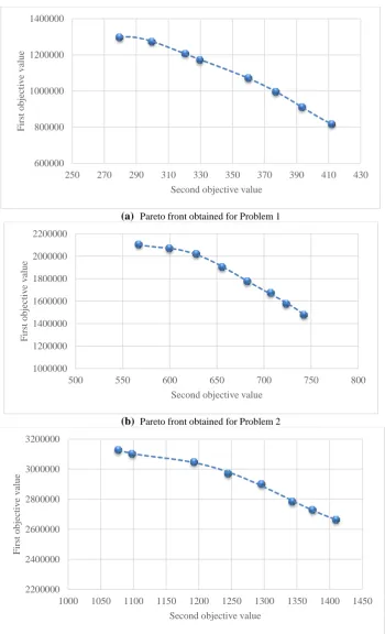
In this section, to evaluate the validity of the problem, three problems with small to large sizes are generated randomly. The input parameters are randomly generated using a uniform distribution. Then the problems are executed on a laptop with Intel Core i7 (8GB of RAM) using CPLEX solver of GAMS software. Information about the random samples generated specified in Table 1. Moreover, the value of the model’s parameters is presented in Table 2. To implement the proposed solution technique, the single-objective problems are solved considering the 1st and 2nd objectives, respectively (cf. Table 3). Then, the breakpoints can be calculated using the obtained values for the 2nd objectives (cf. Table 4). Finally, the problems are solved for each breakpoint based on Problem (53). The Pareto fronts obtained for the problems are depicted in Figure 2. Decision-makers would analyze the obtained Pareto results and choose the best possible solutions according to the trade-off between objectives. To this end, an efficient method, namely, RPA is implemented to extract the best Pareto solution in each problem. The obtained objective values for each solution are represented in Table 2. We should normalize the objective values due to their unit dissimilarity.
Table 1. Information for random instance problems.
|𝑴𝟐|
|𝑴𝟏|
|T| |P|
|𝑽𝑪|
|𝑽𝑺|
|𝑽𝑶|
Problem No.
4 2
6 2
12 4
1 1
5 3
12 4
20 8
2 2
8 5
24 6
30 12
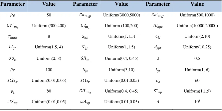
Table 2. Parameters’ value of the proposed model.
Parameter Value Parameter Value Parameter Value
𝑃𝑒 50 𝐶𝑎𝑚1𝑝 Uniform(3000,5000) 𝐶𝑎′𝑚2𝑝 Uniform(500,1000)
𝐶𝑉′
𝑚1 Uniform (300,400) 𝐶𝑉𝑚2 Uniform (100,200) 𝐼𝐶𝑘𝑝𝑡 Uniform(10000,20000)
𝑇𝑚𝑎𝑥 8 𝑆𝑘𝑝 Uniform(1,1.5) 𝐶𝑖𝑗 Uniform(2,10)
𝐿𝐿𝑗𝑡 Uniform(1.5, 4) 𝑆′𝑗𝑝 Uniform(1,1.5) 𝑑𝑗𝑝𝑡 Uniform(10,25)
𝑈𝑈𝑗𝑡 Uniform(2, 8) 𝐺𝐻𝑚1 Uniform(0.4, 0.45) 𝜆 0.5
𝑃𝑒 100 𝑈𝑗𝑡 Uniform(3,10) 𝐿𝑗𝑡 Uniform(1, 6)
𝑠𝑡2𝑘𝑝 Uniform(0.01,0.05) 𝑠𝑡1𝑗𝑝 Uniform(0.01,0.05) 𝑣2 60
𝑣1 80 𝐺𝐻′𝑚2 Uniform(0.4, 0.45) 𝑆′′𝑣𝑝 Uniform(1,1.5)
𝑠𝑡3𝑘𝑝 Uniform(0.01,0.05) 𝑠𝑡4𝑣𝑝 Uniform(0.01,0.05) A 108
Table 3. Computational results for single-objective problems.
Average Run Time (second) Min Obj. 2
Min Obj. 1 Problem No.
Obj. 2 Obj. 1
Obj. 2 Obj. 1
68.504 279.614
1342277.642 419.565
817310.765 1
497.320 566.220
2131605.088 747.114
1477910.497 2
3226.657 1076.690
3206489.761 1459.353
2664148.957 3
Table 4. Different breakpoints in each problem.
Breakpoints Problem No.
7 6
5 4
3 2
1 0
419.565 399.572
379.579 359.586
339.593 319.6
299.607 279.614
1
747.114 721.272
695.43 669.588
643.746 617.904
592.062 566.22
2
1459.353 1404.687
1350.021 1295.355
1240.688 1186.022
1131.356 1076.69
(a) Pareto front obtained for Problem 1
(b) Pareto front obtained for Problem 2
(c) Pareto front obtained for Problem 3
Figure 2. Obtained Pareto fronts for different-sized problems.
As can be seen in Figure 2, there is not a direct relation between two objectives, and the Pareto fronts show a strong contradiction between two objectives. The Pareto frontier in each problem is approximately similar considering it exactness by 8 breakpoints. As it is obvious, we can’t keep both objectives in their optimal levels simultaneously. So, decision-makers should choose only one point among the existing Pareto points. Each point contains different
600000 800000 1000000 1200000 1400000
250 270 290 310 330 350 370 390 410 430
F
irst
o
b
jec
ti
v
e
v
alu
e
Second objective value
1000000 1200000 1400000 1600000 1800000 2000000 2200000
500 550 600 650 700 750 800
F
irst
o
b
jec
ti
v
e
v
alu
e
Second objective value
2200000 2400000 2600000 2800000 3000000 3200000
1000 1050 1100 1150 1200 1250 1300 1350 1400 1450
F
irst
o
b
jec
ti
v
e
v
alu
e
information for the values of decision variables and the main limitations to be institutionalized.
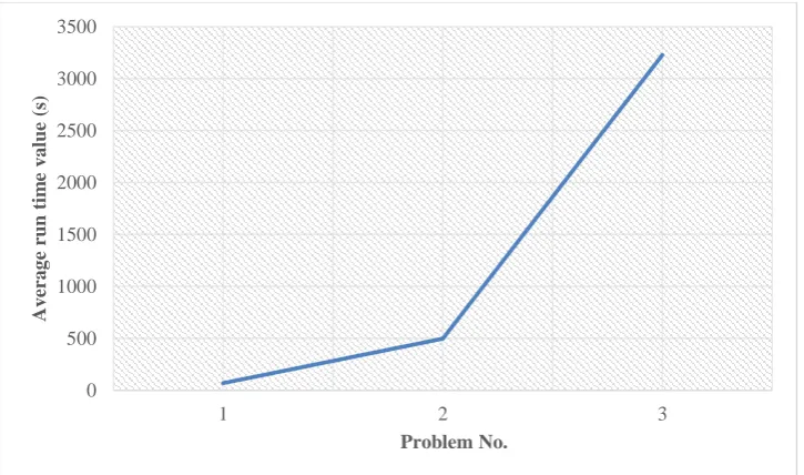
On the other hand, the run time comparison of the problems (cf. Figure 3) demonstrate that the problem has a high complexity such that it may not be solved using exact solution techniques in large scales. Therefore, developing heuristic/meta-heuristic algorithms can be regarded as potential future research directions.
Figure 3. Run time comparison of different problems.
4.1. Best Pareto Solution
This subsection proposes an effective technique to choose the best Pareto solution among the existing ones in the front. Eventually, the selected Pareto solution of each problem can be analyzed and implemented as the optimal planning for 2E-CVRP. Deb and Sundar (2006) introduced RPA to determine the best point or Pareto points in multi-objective problems. This method can be employed by either assigning or not assigning weights to the objectives. The main idea is to identify the solutions which are close to the reference point.
The normalized Euclidean distance (devb) between each non-dominated solutions and the reference point is computed using Eq. (54) so that each solution with the lowest value of
b
dev has the highest priority for the decision-maker.
2
1 max min
1, 2,...,8.
( )
l
l l
L
b l
l l
f z
b
f f
dev w
(54)where wl represents the weight of lth objective in each Pareto solution, fl is the value of objective l, zl denotes the value of the reference objective or reference point, and flmax and
min
l
f are the maximum and minimum values for objective l, respectively. Therefore, to choose the best Pareto solution for each problem, the values of the required parameters are given in Table 5. These values are tuned according to the initial importance of each objective function.
0 500 1000 1500 2000 2500 3000 3500
1 2 3
Av
er
a
g
e
ru
n
tim
e
v
a
lu
e
(s)
Table 5. Parameters’ value in RPA Values Parameters 0.6 1 w 0.4 2 w min 1 1.4 f 1 z min 2 1.3 f 2 z
Maximum value obtained for the first objective among 8 Pareto solutions
max 1 f
Maximum value obtained for the second objective among 8 Pareto solutions
max 2 f
Minimum value obtained value for the first objective among 8 Pareto solutions
min 1 f
Minimum obtained value for the second objective among 8 Pareto solutions
min 2 f
Now, the values obtained for devb of each problem are represented in Table 6. The minimum value obtained for devb in each problem is considered as the best corresponding to its breakpoint number; i.e., Pareto solution number. Finally, Table 7 shows the best Pareto solutions.
Table 6. Values of devbfor each problem.
b
dev of each breakpoint Problem No. 7 6 5 4 3 2 1 0 1.143 1.099 1.082 1.077 1.075 1.089 1.121 1.110 1 1.407 1.380 1.375 1.358 1.377 1.410 1.390 1.367 2 1.602 1.616 1.632 1.709 1.743 1.794 1.797 1.820 3
Table 7. Best Pareto solution for each problem.
Best Pareto Solution Minimum b dev Problem No. Obj. 2 Obj. 1 329.641 1171885.783 1.075 1 682.419 1775074.114 1.358 2 1409.653 2664148.957 1.602 3
5. Conclusion
In this paper, a novel multi-objective mixed-integer linear programming model (MOMILP) is proposed to optimize a green two-echelon capacitated vehicle routing problem (2E-CVRP) of perishable products distribution considering hard and soft time windows. The first echelon includes central depots as suppliers and intermediate depots as central warehouses. The second echelon consists of intermediate depots and customers and the aim is to determine the optimal routes for the vehicles of each echelon. The objectives are to minimize total cost and total CO2 emissions. In order to evaluate the proposed mathematical model, several problems are generated randomly and solved using CPLEX solver of GAMS software. Moreover, the ε-constraint method is applied to the model to cope with its bi-objectiveness. Finally, the obtained Pareto solutions demonstrate an obvious contradictory between two objective functions. Furthermore, an effective technique entitled reference point approach (RPA) is then implemented to help the decision-maker for finding the best Pareto solution in each problem.
For future studies, meta-heuristic algorithms can be employed to solve the large-sized problems in reasonable run times, and we may include the other objectives such as reliability maximization, minimization of total service time. Moreover, some real assumptions can be incorporated in the model such as urban traffic conditions to make the model more close to the real-world.
References
Alinaghian, M., Amanipour, H., and Tirkolaee, E.B., (2014). "Enhancement of Inventory Management Approaches in “Vehicle Routing-Cross Docking” Problems", Journal of Supply Chain Management Systems, Vol. 3, No. 3.
Babaee Tirkolaee, E., Alinaghian, M., Bakhshi Sasi, M., and Seyyed Esfahani, M., (2016). "Solving a robust capacitated arc routing problem using a hybrid simulated annealing algorithm: a waste collection application", Journal of Industrial Engineering and Management Studies, Vol. 3, pp. 61-76.
Babaee Tirkolaee, E., Abbasian, P., Soltani, M., and Ghaffarian, S.A., (2019). "Developing an applied algorithm for multi-trip vehicle routing problem with time windows in urban waste collection: A case study. ", Waste Management & Research, Vol. 37, pp. 4-13.
Bérubé, J.F., Gendreau, M., and Potvin, J.Y., (2009). "An exact ϵ-constraint method for bi-objective combinatorial optimization problems: Application to the Traveling Salesman Problem with Profits", European Journal of Operational Research, Vol. 194, No. 1, pp. 39-50.
Chen, H.-K., Hsueh, C.-F., and Chang, M.-S., (2009). "Production scheduling and vehicle routing with time windows for perishable food products", Computers and Operations Research, Vol. 36, pp. 72311-2319.
Crainic, T.G., Mancini, S., Perboli, G., and Tadei, R., (2012). "Impact of generalized travel costs on satellite location in the two-echelon vehicle routing problem", Procedia-Social and Behavioral Sciences, Vol. 39, pp. 195-204.
Dantzig, G.B., and Ramser, J., (1959). "The truck dispatching problem", Management Science, Vol. 6, No. 1, pp. 80–91.
Ehrgott, M., and Gandibleux, X., (2003). "Multiobjective combinatorial optimization-theory, methodology, and applications", In Multiple criteria optimization: State of the art annotated bibliographic surveys (pp. 369-444). Springer US.
Esmaili, M., and Sahraeian, R., (2017). "A new Bi-objective model for a Two-echelon Capacitated Vehicle Routing Problem for Perishable Products with the Environmental Factor", International Journal of Engineering, Vol. 30, No. 4, pp. 523-531.
Franceschetti, A., Honhon, D., Van Woensel, T., Bektaş, T., and Laporte, G., (2013). "The time-dependent pollution-routing problem", Transportation Research Part B: Methodological, Vol. 56, pp. 265-293.
Goli, A., Babaee Tirkolaee, E., and Soltani, M., (2019a). "A robust just-in-time flow shop scheduling problem with outsourcing option on subcontractors", Production & Manufacturing Research, Vol. 7, No. 1, pp. 294-315.
Goli, A., Tirkolaee, E.B., Malmir, B., Bian, G.B., and Sangaiah, A.K., (2019b). "A multi-objective invasive weed optimization algorithm for robust aggregate production planning under uncertain seasonal demand", Computing, Vol. 101, No. 6, pp. 499-529.
Golpîra, H., (2016). "A robust bi-objective uncertain green supply chain network management", Serbian Journal of Management, Vol. 11, No. 2, pp. 211-222.
Golpîra, H., (2017a). "Supply chain network design optimization with risk-averse retailer", International Journal of Information Systems and Supply Chain Management (IJISSCM), Vol. 10, No. 1, pp. 16-28.
Golpîra, H., (2017b). "Robust bi-level optimization for an opportunistic supply chain network design problem in an uncertain and risky environment", Operations Research and Decisions, Vol. 27.
Golpîra, H., Zandieh, M., Najafi, E., and Sadi-Nezhad, S., (2017a). "A multi-objective, multi-echelon green supply chain network design problem with risk-averse retailers in an uncertain environment", Scientia Iranica. Transaction E, Industrial Engineering, Vol. 24, No. 1, p. 413.
Golpîra, H., Najafi, E., Zandieh, M., and Sadi-Nezhad, S., (2017b). "Robust bi-level optimization for green opportunistic supply chain network design problem against uncertainty and environmental risk", Computers and Industrial Engineering, Vol. 107, pp. 301-312.
Golpîra, H., (2019). "Optimal Integration of the Facility Location Problem into the Multi-Project Multi-Supplier Multi-Resource Construction Supply Chain Network Design under the Vendor Managed Inventory Strategy", Expert Systems with Applications.
Jabali, O., Woensel, T., and de Kok, A., (2012). "Analysis of travel times and CO2 emissions in time‐dependent vehicle routing", Production and Operations Management, Vol. 21, No. 6, pp. 1060-1074.
Khan, S.A.R., Zhang, Y., Anees, M., Golpîra, H., Lahmar, A., and Qianli, D., (2018). "Green supply chain management, economic growth and environment: A GMM based evidence", Journal of Cleaner Production, Vol. 185, pp. 588-599.
Khan, S.A.R., Chen, J., Zhang, Y., and Golpîra, H., (2019a). "Effect of green purchasing, green logistics, and ecological design on organizational performance: A path analysis using structural equation modeling", Information Technology and Intelligent Transportation Systems, pp. 183-190.
Khan, S. A. R., Jian, C., Zhang, Y., Golpîra, H., Kumar, A., and Sharif, A., (2019c). "Environmental, social and economic growth indicators spur logistics performance: From the perspective of South Asian Association for Regional Cooperation countries", Journal of cleaner production, Vol. 214, pp. 1011-1023.
Kritikos, M.N., and Ioannou, G., (2013). "The heterogeneous fleet vehicle routing problem with overloads and time windows", International Journal of Production Economics, Vol. 144, pp. 168-75.
Mandziuk, J., and Swiechowski, M., (2017). "UCT in Capacitated Vehicle Routing Problem with traffic jams", Information Sciences, pp. 42–56.
Marandi, F., (2017). "A new approach in graph-based integrated production and distribution scheduling for perishable products", Journal of Quality Engineering and Production Optimization, Vol. 2, No. 1, pp. 65-76.
Mostafaeipour, A., Qolipour, M., Rezaei, M., and Babaee-Tirkolaee, E., (2019). "Investigation of off-grid photovoltaic systems for a reverse osmosis desalination system: A case study", Desalination, Vol. 454, pp. 91-103.
Perboli, G., Tadei, R. and Vigo, D., (2011). "The two-echelon capacitated vehicle routing problem: Models and math-based heuristics", Transportation Science, Vol. 45, No. 3, pp. 364-380.
Rahbari, A., Nasiri, M.M., Werner, F., Musavi, M., and Jolai, F., (2019). "The vehicle routing and scheduling problem with cross-docking for perishable products under uncertainty: Two robust bi-objective models", Applied Mathematical Modelling, Vol. 70, pp. 605-625.
Rohmer, S.U.K., Claassen, G.D.H., and Laporte, G., (2019). "A two-echelon inventory routing problem for perishable products", Computers & Operations Research, Vol. 107, pp. 156-172.
Sangaiah, A. K., Tirkolaee, E.B., Goli, A., and Dehnavi-Arani, S., (2019). "Robust optimization and mixed-integer linear programming model for LNG supply chain planning problem", Soft Computing, pp. 1-21.
Song, B.D., and Ko, Y.D., (2016). "A vehicle routing problem of both refrigerated-and general-type vehicles for perishable food products delivery", Journal of Food Engineering, Vol. 169, No. 3, pp. 61-71.
Soysal, M., Bloemhof-Ruwaard, J. M., and Bektaş, T., (2015). "The time-dependent two-echelon capacitated vehicle routing problem with environmental considerations", International Journal of Production Economics, Vol. 164, pp. 366-378.
Tirkolaee E.B., Goli, A., Bakhshi, M., and Mahdavi, I., (2017). "Robust Multi-Trip Vehicle Routing Problem of Perishable Products with Intermediate Depots and Time Windows", Numerical Algebra Control and Optimization, Vol. 7, No. 4, pp. 417-433.
Tirkolaee, E.B., Mahdavi, I., and Esfahani, M.M.S., (2018a). "A robust periodic capacitated arc routing problem for urban waste collection considering drivers and crew’s working time", Waste Management, Vol. 76, pp. 138-146.
Tirkolaee, E.B., Alinaghian, M., Hosseinabadi, A.A.R., Sasi, M. B., and Sangaiah, A. K., (2018b). "An improved ant colony optimization for the multi-trip Capacitated Arc Routing Problem", Computers and Electrical Engineering.
Tirkolaee, E.B., Goli, A., Hematian, M., Sangaiah, A.K., and Han, T. (2019a). "Multi-objective multi-mode resource constrained project scheduling problem using Pareto-based algorithms", Computing, Vol. 101, No. 6, pp. 547-570.
Tirkolaee, E.B., Goli, A., and Weber, G.W., (2019b). "Multi-objective Aggregate Production Planning Model Considering Overtime and Outsourcing Options Under Fuzzy Seasonal Demand", In Advances in Manufacturing II (pp. 81-96). Springer, Cham.
Tirkolaee, E.B., Mahmoodkhani, J., Bourani, M.R., and Tavakkoli-Moghaddam, R., (2019c). "A Self-Learning Particle Swarm Optimization for Robust Multi-Echelon Capacitated Location-Allocation-Inventory Problem", Journal of Advanced Manufacturing Systems.
Wang, K., Shao, Y., and Zhou, W., (2017). "Metaheuristic for a two-echelon capacitated vehicle routing problem with environmental considerations in city logistics service", Transportation Research Part D: Transport and Environment, Vol. 57, pp. 262-276.
Yavari, M., and Zaker, H., (2019). "An integrated two-layer network model for designing a resilient green-closed loop supply chain of perishable products under disruption", Journal of Cleaner Production, Vol. 230, pp. 198-218.
Yavari, M., and Geraeli, M., (2019). "Heuristic method for robust optimization model for green closed-loop supply chain network design of perishable goods", Journal of Cleaner Production, Vol. 226, pp. 282-305.
Yu, Z., Golpîra, H., and Khan, S. A., (2018). "The relationship between green supply chain performance, energy demand, economic growth and environmental sustainability: An empirical evidence from developed countries", LogForum, Vol. 14, No. 4.
Zhou, L., Baldacci, R., Vigo, D., and Wang, X., (2018). "A multi-depot two-echelon vehicle routing problem with delivery options arising in the last mile distribution", European Journal of Operational Research, Vol. 265, No. 2, pp. 765-778.
This article can be cited: Babaee Tirkolaee, E., Hadian, Sh., Golpîra, H., (2019). "A novel multi-objective model for two-echelon green routing problem of perishable products with intermediate depots", Journal of Industrial Engineering and Management Studies, Vol. 6, No. 2, pp. 196-213.