Model-free Nonconvex Matrix Completion: Local Minima
Analysis and Applications in Memory-efficient Kernel PCA
Ji Chen [email protected]
Department of Mathematics University of California, Davis Davis, CA 95616, USA
Xiaodong Li [email protected]
Department of Statistics University of California, Davis Davis, CA 95616, USA
Editor:Benjamin Recht
Abstract
This work studies low-rank approximation of a positive semidefinite matrix from partial entries via nonconvex optimization. We characterized how well local-minimum based low-rank factorization approximates a fixed positive semidefinite matrix without any assump-tions on the rank-matching, the condition number or eigenspace incoherence parameter. Furthermore, under certain assumptions on rank-matching and well-boundedness of con-dition numbers and eigenspace incoherence parameters, a corollary of our main theorem improves the state-of-the-art sampling rate results for nonconvex matrix completion with no spurious local minima inGe et al.(2016,2017). In addition, we have investigated when the proposed nonconvex optimization results in accurate low-rank approximations even in presence of large condition numbers, large incoherence parameters, or rank mismatching. We also propose to apply the nonconvex optimization to memory-efficient kernel PCA. Compared to the well-known Nystr¨om methods, numerical experiments indicate that the proposed nonconvex optimization approach yields more stable results in both low-rank approximation and clustering.
Keywords: low-rank approximation, matrix completion, nonconvex optimization, model-free analysis, local minimum analysis, kernel PCA
1. Introduction
Let M be an n×n positive semidefinite matrix and let r n be a fixed integer. It is well known that a rank-r approximation of M can be obtained by truncating the spectral decomposition of M. To be specific, letM =Pn
i=1σiuiu>i be the spectral decomposition withσ1 >. . .>σn>0. Then, the best rank-r approximation ofM isMr=Pri=1σiuiu>i . If we denote Ur = [
√
σ1u1 . . . √
σrur], then the best rank-r approximation of M can be written as M = UrUr>. By the well-known Eckart-Young-Mirsky Theorem (Golub and Van Loan,2012), Ur is actually the global minimum (up to rotation) to the following nonconvex optimization:
min
X∈Rn×rkXX
>−Mk2
F.
c
This factorization for low-rank approximation has been well-known in the literature (see, e.g., Burer and Monteiro,2003).
This paper studies how to find a rank-rapproximation ofM in the case that only partial entries are observed. Let Ω⊂[n]×[n] be a symmetric index set, and we assume thatM
is only observed on the entries in Ω. For convenience of discussion, this subsampling is represented asPΩ(M) in thatPΩ(M)i,j =Mi,j if (i, j)∈Ω andPΩ(M)i,j = 0 if (i, j)∈/ Ω. We are interested in the following question
How to find a rank-r approximation of M in a scalable manner only through PΩ(M)?
We propose to find such a low-rank approximation through the following nonconvex op-timization, which has been exactly proposed inGe et al.(2016,2017) for matrix completion. DenoteX =x1, . . . ,xn
>
∈Rn×r. A rank-r approximation of M can be found through
min
X∈Rn×rf(X) := 1 2
X
(i,j)∈Ω
x>i xj−Mij
2
+λ n
X
i=1
[(kxik2−α)+]4
:= 1
2kPΩ(XX
>−M)k2
F +λGα(X) (1)
whereGα(X) :=Pn
i=1[(kxik2−α)+]4. Following the framework of nonconvex optimization
without initialization inGe et al.(2016,2017), our local-minimum based approximation for
M isM ≈XcXc> where Xcisany local minimum of (1).
Let’s briefly discuss the memory and computational complexity to solve (1) via gradient descent. If Ω is symmetric and does not contain the diagonal entries as later specified in Definition1, the updating rule of gradient decent
X(t+1) =X(t)−η(t)∇f(X(t)) (2) is equivalent to
x(t+1)i :=x(t)i −η(t)
2
X
j:(i,j)∈Ω
hx(t)i ,x(t)j i −Mi,j
x(t)j + 4λ
kx(t)i k2
kx(t)i k2−α
3
1{kx(t) i k2>α}x
(t) i
,
where the memory cost is dominated by storing X(t), X(t+1), and M on Ω, which is generally O(nr+|Ω|). It is also obvious that the computational cost in each iteration is O(|Ω|r).
1.1. Applications in memory-efficient kernel PCA
However, when the sample size is large, the storage of the kernel matrix itself becomes challenging. Consider the example when the dimension dis in thousands while the sample sizenis in millions. The memory cost for the data matrix isd×nand thus in billions, while the memory cost for the kernel matrix M is in trillions! On the other hand, if not storing
M, the implementation of standard iterative algorithms of SVD will involve one pass of computing all entries of M in each iteration, usually with formidable computational cost O(n2d). A natural question arises: How to find low-rank approximations of M memory-efficiently?
The following two are among the most well-known memory-efficient kernel PCA meth-ods in the literature. One is Nystr¨om method (Williams and Seeger,2001), which amounts to generatingrandom partial columns of the kernel matrix, then finding a low-rank approx-imation based on these columns. In order to generate random partial columns, uniform sampling without replacement is employed in Williams and Seeger (2001), and different sampling strategies are proposed later (e.g., Drineas and Mahoney,2005). The method is convenient in implementation and efficient in both memory and computation, but relatively unstable in terms of approximation errors as will be shown in Section 3.
Another popular approach is stochastic approximation, e.g., Kernel Hebbian Algorithm (KHA) (Kim et al., 2005), which is memory-efficient and approaches the exact principal component solution as the number of iterations goes to infinity with appropriately chosen learning rate (Kim et al., 2005). However, based on our experience, the method usually requires careful tuning of learning rates even for very slow convergence.
It is also worth mentioning that the randomized one-pass algorithm discussed in, e.g., Halko et al.(2011), where the theoretical properties of a random-projection based low-rank approximation method were fully analyzed. However, although the one-pass algorithm does not require the storage of the whole matrix M, in kernel PCA one still needs to compute every entry of M, which typically requires O(n2d) computational complexity for kernel matrix.
As a result, we aim at finding a memory-efficient method as an alternative to the afore-mentioned approaches. In particular, we are interested in a method with desirable empirical properties: memory-efficient, no requirement on one or multiple passes to compute the com-plete kernel matrix, no requirement to tune the parameters carefully, and yielding stable results. To this end, we propose the following method based on entries sampling and non-convex optimization: In the first step, Ω is generated to follow an Erd˝os-R´enyi random graph with parameter p later specified in Definition 1, and then a partial kernel matrix PΩ(M) is generated in that Mi,j =K(zi,zj) for (i, j) ∈ Ω. In the second step, the non-convex optimization (1) is implemented through gradient descent (2). Any local minimum of (1), Xb, is a solution of approximate kernel PCA in thatM ≈XbXb>.
To store the index set Ω and the sampled entries of M on Ω, the memory cost in the first step isO(|Ω|), which is comparable to the memory costO(nr+|Ω|) in the second step. As to the computational complexity, besides the generation of Ω, the computational cost in the first step is typicallyO(|Ω|d), e.g., when the radial kernels or polynomial kernels are employed. This could be dominating the per-iteration computational complexity O(|Ω|r) in the second step when the target rank r is much smaller than the original dimensiond.
of our knowledge, our work is the first to apply such an idea to memory-efficient kernel PCA. Moreover, the underlying signal matrix is assumed to be exactly low-rank in Yi et al.(2016) while we make no assumptions on the positive semidefinite kernel matrix M. Entry-sampling has been proposed in Achlioptas et al. (2002); Achlioptas and McSherry (2007) for scalable low-rank approximation. In particular, it is used to speed up kernel PCA in Achlioptas et al. (2002), but spectral methods are subsequently employed after entries sampling as opposed to nonconvex optimization. Empirical comparisons between spectral methods and nonconvex optimization will be demonstrated in Section 3. It is also noteworthy that matrix completion techniques have been applied to certain kernel matrices when it is costly to generate each single entry (Graepel,2002; Paisley and Carin, 2010), wherein the proposed methods are not memory-efficient. In contrast, our method is memory-efficient in order to serve a different purpose.
1.2. Related work and our contributions
In recent years, a series of papers have been proposed to study nonconvex matrix completion (see, e.g., Rennie and Srebro,2005;Keshavan et al.,2010b,a;Jain et al.,2013;Zhao et al., 2015;Sun and Luo,2016;Chen and Wainwright,2015;Yi et al.,2016;Zheng and Lafferty, 2016;Ge et al.,2016,2017). Interested readers are referred toBalcan et al. (2017), where required sampling rates in these papers are summarized in Table 1 therein. Compared to convex approaches for matrix completion (e.g.,Cand`es and Recht,2009), these nonconvex approaches are not only more computationally efficient, but also more convenient in storing. For the same reason, nonconvex optimization approaches have also been investigated for other low-rank recovery problems including phase retirval (e.g., Candes et al., 2015; Sun et al., 2018; Cai et al., 2016), matrix sensing (e.g., Zheng and Lafferty, 2015; Tu et al., 2015), blind deconvolution (e.g.,Li et al.,2018), etc.
c
XXc>, as long as M is exactly rank-r, the condition numberκr:=σ1/σr is well-bounded,
the incoherence parameter of the eigenspace of M is well-bounded, and the sampling rate is greater than a function of these quantities. The case with additive stochastic noise has also been discussed in Ge et al.(2016).
In contrast, our paper studies the theoretical properties of XcXc> withno assumptions
on M. There are actually two questions of interest: how close XcXc> is from M, and
how close XcXc> is from Mr (recall that Mr is the best rank-r approximation of M by
spectral truncation). In comparison toGe et al. (2016,2017), our main contributions to be introduced in the next section include the following:
• Our main result Theorem2that characterizes how well any local-minimum based rank-rfactorizationXcXc>approximatesM orMrrequires no assumptions imposed onM
regarding its rank, eigenvalues and eigenvectors. The sampling rate is only required to satisfyp>C(logn/n) for some absolute constant C. Therefore, for applications such as memory-efficient kernel PCA, our framework provides more suitable guidelines than Ge et al. (2016, 2017). In fact, kernel matrices are in general of full rank and their condition numbers and incoherence parameters may not satisfy the strong assumptions inGe et al.(2016,2017).
• When M is assumed to be exactly low-rank as in Ge et al. (2016, 2017), Corollary
3 improves the state-of-the-art no-spurious-local-minima results in Ge et al. (2016, 2017) for exact nonconvex matrix completion in terms of sampling rates. To be specific, assuming both condition numbers and incoherence parameters are on the order of O(1), our result improves the result in Ge et al. (2017) from Oe(r4/n) to
e
O(r2/n).
• Theorem 2 also implies the conditions under which the nonconvex optimization (1) yields good low-rank approximation of M in the cases of large condition numbers, high incoherence parameters, or rank-mismatching.
On the other hand, our paper benefits from Ge et al. (2016, 2017) in various aspects. In order to characterize the properties of any local minimum Xc, we follow the idea in Ge
et al. (2017) to combine the first and second order conditions of local minima linearly to construct an auxiliary function, denoted as K(X) in our paper, and consequently all local minima satisfy the inequality K(Xc)>0 as illustrated in Figure 1. If M is exactly rank-r
and its eigenvalues and eigenvectors satisfy particular properties, Ge et al. (2017) shows that K(X)60 for all X as long as the sampling rate is large enough. This argument can be employed to prove that there is no spurious local minima.
However, K(X)6 0 does not hold for allX if no assumptions are imposed on M, so we instead focus on analyzing the inequality K(Xc)>0 directly in the model-free manner.
K(X)
−f(X)
Ur
span of local minima
of f(X)
span of {X ∈Rn×r|K(X)>0}
Figure 1: Landscape of−f(X), K(X) and Ur.
1.3. Organization and notations
The remainder of the paper is organized as follows: Our main theoretical results are stated in Section 2; Numerical simulations and applications in memory-efficient KPCA are given in Section3. Proofs are deferred to Section4.
We use bold letters to denote matrices and vectors. For any vectors u and v, kuk2 denotes its `2 norm, and hu,vi their inner product. For any matrix M ∈ Rn×n, Mi,j denotes its (i, j)-th entry, Mi,· = (Mi,1, Mi,2, . . . , Mi,n)> its i-th row of M, and M·,j = (M1,j, M2,j, . . . , Mn,j)>itsj-th column. Moreover, we usekMk,kMk∗,kMkF,kMk`∞ :=
maxi,j|Mi,j|,kMk2,∞:= maxikMi,·k2to denote its spectral norm, nuclear norm, Frobenius norm, elementwise max norm and `2,∞ norm, respectively. The vectorization of M is
represented by vec(M) = (M1,1, M2,1, . . . , M1,2, . . . , Mn,n)>. For matrices M,N of the same size, denote hM,Ni =P
i,jMi,jNi,j = trace M>N
. Denote by ∇f(M) ∈ Rn×n and ∇2f(M)∈
Rn2×n2 the gradient and Hessian of f(M).
Denote [x]+ = max{x,0}. We use J to denote a matrix whose all entries equal to one. We use C, C1, C2, . . . to denote absolute constants, whose values may change from line to line.
2. Model-free approximation theory
2.1. Main results
Definition 1 (Off-diagonal symmetric independent Ber(p) model) Assume the in-dex setΩ consists only of off-diagonal entries that are sampled symmetrically and indepen-dently with probability p, i.e.,
1. (i, i)∈/Ω for alli= 1, . . . , n;
2. For all i < j, sample (i, j)∈Ωindependently with probability p; 3. For all i > j, (i, j)∈Ω if and only if (j, i)∈Ω.
Here we assume all diagonal entries are not in Ω for the generality of the formulation, although they are likely to be obtained in practice. For instance, all diagonal entries of the radial kernel matrix are ones. For any index set Ω ⊂ [n]×[n], define the associated 0-1 matrix Ω ∈ {0,1}n×n such that Ω
i,j = 1 if and only if (i, j) ∈Ω. Then we can write PΩ(X) =X◦Ωwhere◦ is the Hadamard product.
Assume that the positive semidefinite matrix M has the spectral decomposition
M =
r
X
i=1
σiuiu>i + n
X
i=r+1
σiuiu>i :=Mr+N, (3)
where σ1 > σ2 >· · · > σn > 0 are the spectrum, ui ∈Rn are unit and mutually
perpen-dicular eigenvectors. The matrix Mr := Pri=1σiuiu>i is the best rank-r approximation of
M andN :=Pn
i=r+1σiuiu
>
i denotes the residual part. In the case of multiple eigenvalues, the order in the eigenvalue decomposition (3) may not be unique. In this case, we consider the problem for any fixed order in (3) with the fixed Mr.
Theorem 2 Let M ∈Rn×n be a positive semidefinite matrix with the spectral
decomposi-tion (3). Let Ωbe sampled according to the off-diagonal symmetric Ber(p) model withp> CSlognn for some absolute constantCS. Then in an eventE with probabilityP[E]>1−2n−3,
as long as the tuning parameters α and λ satisfy 100pkMrk`∞ 6α 6200
p
kMrk`∞ and
100kΩ−pJk6λ6200kΩ−pJk, any local minimum Xc∈Rn×r of (1) satisfies
XcXc
>−M
r
2 F 6C1
r
X
i=1
(
C2
rn
p + logn
p
kMrk`∞+C2σ2r+1−i−σi
+
)2
+C1
[p(1−p)n+ logn]rkNk2 `∞
p2
(4)
and
XcXc
>−M
2 F 6C1
r
X
i=1
(
C2
rn
p + logn
p
kMrk`∞+C2σ2r+1−i−σi
+
)2
+C1
[p(1−p)n+ logn]rkNk2 `∞
p2 +kNk
2 F
(5)
Model-free low-rank approximation from partial entries has been studied for for spectral estimators in the literature. For example, under the settings of Theorem 2, the spectral low-rank approximation (denoted asMapprox) discussed inKeshavan et al.(2010a, Theorem 1.1) is guaranteed to satisfy
kMapprox−Mrk2F 6C
(
nrkMrk2`∞
p +
rkPΩ(N)k2 p2
)
,
with high probability. However, this cannot imply exact recovery even when M is of low rank and the sampling ratepsatisfies the conditions specified inGe et al.(2017). Similarly, the SVD-based USVT estimator introduced in Chatterjee (2015) does not imply exact recovery. In contrast, as will be discussed in the next subsection, Theorem 2 implies that any local minimum of (1) yields exact recovery of M with high probability under milder conditions than those inGe et al. (2017).
2.2. Implications in exact matrix completion
Assume in this subsection that the positive semidefinite matrixM is exactly rank-r, i.e.,
M =Mr =
r
X
i=1
σiuiu>i =UrUr> (6)
where Ur = [ √
σ1u1 . . . √
σrur]. Furthermore, we assume its condition number κr = σ1σr and eigen-space incoherence parameterµr = nrmaxiPrj=1u2i,j(Cand`es and Recht,2009) are well-bounded. This is a standard setup in the literature of nonconvex matrix completion (e.g., Keshavan et al.,2010b; Sun and Luo, 2016; Chen and Wainwright,2015;Zheng and Lafferty,2016;Ge et al.,2016;Yi et al.,2016;Ge et al.,2017).
Notice that Ge et al. (2016) introduces a slightly different version of incoherence
e
µr:= √
nkUrk2,∞
kUrkF =
s
nkMrk`∞
trace(Mr)
(7)
as a measure of spikiness. (Note that this is different from the spikiness defined in Negah-ban and Wainwright (2012).) By kMrk`∞ = kUrk22,∞ = maxi
Pr
j=1σju2i,j, the following relationship betweenµ and eµis straightforward
e
µ2r κr 6
e
µ2rtrace(Mr) rσ1
= nkMrk`∞
rσ1 6 µr6
nkMrk`∞
rσr
= µe
2
rtrace(Mr) rσr 6
κrµe
2
r. (8)
By the fact kMk`∞ 6
r
nσ1µr, Theorem2implies the following exact low-rank recovery results:
Corollary 3 Under the assumptions of Theorem 2, if we further assume rank(M) = r
(i.e., M =Mr) and
p>Cmax
µrrκrlogn
n ,
µ2rr2κ2r n
or
p>Cmax
e
µ2rrκrlogn
n ,
e
µ4rr2κ2r n
for some absolute constant C, then in an event E with probability P[E] > 1−2n−3, any
local minimum Xc∈Rn×r of objective function f(X) defined in (1) satisfies XcXc>=M.
The proof is straightforward and deferred to the appendix. Notice that our results are better than the state-of-the-art results for no spurious local minimum in Ge et al. (2017), where the required sampling rate is p> Cnµ3rr4κ4rlogn (which also implies p > Cnµe
6
rr4κ7rlogn by (8)).
2.3. Examples
Besides improving the state-of-the-art no-spurious-local-minima results in nonconvex matrix completion, Theorem2is also capable of explaining some nontrivial phenomena in low-rank matrix completion in the presence of large condition numbers, high incoherence parameter, or mismatching between the selected and true ranks.
2.3.1. Nonconvex matrix completion with large condition numbers and high eigen-space incoherence parameters
Assume here M is exactly rank-r and its spectral decomposition is denoted as in (6). However, we assume that µr and κr can be extremely large, while the condition num-ber and incoherence parameter for Mr−1 = Pri=1−1σiuiui>, i.e., κr−1 = σrσ1−1 and µr−1 =
n r−1maxi
Pr−1
j=1u2i,j, are well-bounded. We are interested in figuring out when the local minimum based rank-r factorizationXcXc> approximates the original M well.
By kMrk`∞ = maxi
Pr
j=1σju2i,j, we have kMrk`∞ 6
r−1
n σ1µr−1+σrkurk 2
∞.
Then by Theorem 2, if
p>Cmax
h
µr−1κr−1(r−1) +nσrσr−1kurk2∞ i
logn
n ,
h
µr−1κr−1(r−1) +nσrσr−1kurk2∞ i2
n
with some absolute constant C, in an event E with probability P[E]> 1−2n−3, for any
local minimum Xc ∈ Rn×r of (1), kXcXc>−Mk2F 6 1001 σ2r−1 holds. In other words, the
relative approximation error satisfies RE:= kXcXc>−MkF
kMkF 6
1 10√r−1. Notice that kurk2∞ 6 nrµr and
σr σr−1 =
κr−1
κr , so the above sampling rate requirement is satisfied as long as µrκr 6Cµr−1 and
p>Cmax
µr−1κr−1rlogn
n ,
µ2r−1κ2r−1r2 n
2.3.2. Rank mismatching
In this subsection,M is assumed to be exactly rank-R, i.e.,
M =MR=
R
X
i=1
σiuiu>i =URUR>
where UR = [ √
σ1u1 . . . √
σRuR]. However, we consider the case that the selected rank r is not the same as the true rank R, i.e., rank mismatching. As with Section
2.2, we assume the condition number κR = σRσ1 and eigen-space incoherence parameter
µR= RnmaxiPRj=1σju2i,j are well-bounded. As with (8), there holdskMk`∞ 6
R nσ1µR.
Case 1: R < r. Theorem2 implies that if
p>Cmax
µRκRRlogn
n ,
µ2Rκ2RR2 n
for some absolute constant C, then in an event E with probability P[E] >1−2n−3, any
local minimumXc∈Rn×r of (1) yieldskXcXc>−Mk2F 6 1001 (r−R)σR2. This further yields
the relative approximation error boundRE:= kXcXc>−MkF
kMkF 6
1 10
q
r−R R .
Case 2: R > r. Recall that kMrk`∞ 6
r
nσ1µr. Moreover,
kNk`∞ = max i
R
X
j=r+1
σju2i,j 6σr+1
max
i R
X
j=1 u2i,j
=
µRR n σr+1.
Theorem2 implies that if
p>Cmax
µrrκrlogn
n ,
µ2rr2κ2r n ,
µ2RR3 n
for some absolute constant C, then with high probability, any local minimum Xc∈Rn×r of
(1) yields
kXcXc>−Mrk2F 6C(σ2r+1+. . .+σ2r2 ),
which implies that the relative error is well-controlled as long as σr+12 +. . .+σR2 accounts for a small proportion inσ12+. . .+σ2R.
If we assume that 2C2σr+1 < σr where C2 is specified in Theorem 2, under the same sampling rate requirement as above, Theorem2 implies a much sharper result:
kXcXc>−Mrk2F 6 1 100σ
2 r+1,
which yields the following (perhaps surprising) relative approximation error bound
RE:= kXcXc
>−M
rkF kMrkF 6
1 10
s
σ2r+1 σ2
1 +. . .+σ2r 6 1
3. Experiments
In the following simulations where the nonconvex optimization (1) is solved, the initializa-tion X(0) is constructed randomly with i.i.d. normal entries with mean 0 and variance 1. The step sizeη(t)for the gradient descent (2) is determined by Armijo’s rule (Armijo,1966). The gradient descent algorithm is implemented with sparse matrix storage in Section3.2for the purpose of memory-efficient KPCA, while with full matrix storage in Section3.1to test the performance of general low-rank approximations from missing data. In each experiment, the iterations will be terminated when k∇f(X(t))kF 6 10−3 or kη(t)∇f(X(t))kF 610−10 or the number of iterations surpasses 103. All methods are implemented in MATLAB. The experiments are running on a virtual computer with Linux KVM, with 12 cores of 2.00GHz Intel Xeon E5 processor and 16 GB memory.
3.1. Numerical simulations
In this section, we conduct numerical tests on the nonconvex optimization (1) under different settings of spectrum for the 500×500 positive semidefinite matrixM, whose eigenvectors are the same as the left singular vectors of a random 500×500 matrix with i.i.d. standard normal entries. The generation of eigenvalues for M will be further specified in each test. For each generated M, the nonconvex optimization (1) is implemented for 50 times with independent Ω’s generated under the off-diagonal symmetric independent Ber(p) model. To implement the gradient descent algorithm (2), set α = 100kMk`∞ and λ= 100kΩ− pJk (the performances of our method are empirically not sensitive to the choices of the tuning parameters). In each single numerical experiment, we also conduct spectral method proposed in Achlioptas et al. (2002) to obtain an approximate low-rank approximation of
M for the purpose of comparison.
3.1.1. Full rank case
Here M is assumed to have full rank, i.e., rank(M) = 500. To be specific, let σ1 =· · ·= σ4 = 10, σ6 = · · · = σ500 = 1, and σ5 = 10,9,8, . . . ,2,1. The selected rank used in the nonconvex optimization (1) is set as r = 5, and the sampling rate is set as p = 0.2. With different values of σ5, the results of our implementations of the gradient descent are plotted in Figure 2. One can observe that the relative errors for our nonconvex method (1) are well-bounded for different σ5’s, and much smaller than those for spectral low-rank approximation. The results indicate that our approach is able to approximate the “true” best rank-rapproximationMr accurately in the presence of heavy spectral tail and possibly large condition numberσ1/σ5, even with only 20% observed entries.
3.1.2. Low-rank matrix with large condition numbers
10 9 8 7 6 5 4 3 2 1
5
0 0.1 0.2 0.3 0.4 0.5 0.6
relative error
nonconvex method spectral method median of nonconvex method median of spectral method
(a) Relative error kMapprox−MrkF kMrkF .
10 9 8 7 6 5 4 3 2 1
5
0.7 0.72 0.74 0.76 0.78 0.8 0.82
relative error
nonconvex method spectral method best rank r approximation median of nonconvex method median of spectral method
(b) Relative error kMapprox−MkF kMkF .
Figure 2: Relative errors for full rank case.
10 20 30 40 50 100 200 condition number
0 0.1 0.2 0.3 0.4 0.5 0.6
relative error
nonconvex method spectral method median of nonconvex method median of spectral method
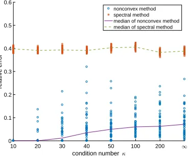
Figure 3: Relative error kMapprox−MkF
kMkF for low-rank matrix with extreme condition numbers.
The performance of our nonconvex approach with various choices ofκis demonstrated in Figure 3. One can observe that our nononvex optimization approach yields exact recovery ofM whenκ= 10, while yields accurate low-rank approximation forM with relative errors almost always smaller than 0.3 when κ >20. This fact is consistent with the example we discussed in Section 2.3.1, where we have shown that under certain incoherence conditions, the relative approximation error can be well-bounded even whenκr =∞.
3.1.3. Rank mismatching
rank from 1 to 15, while the selected rank is always r = 5. The sampling rate is fixed as p = 0.2. We perform the simulation on two sets of spectrums: For the first one, all the nonzero eigenvalues are 10; And the second one has decreasing eigenvalues: σ1 = 20, σ2 = 18,· · ·, σ10= 2 for the case of fixed rank(M), σ1 = 30,· · ·, σrank(M) = 32−2×rank(M) for the case of fixed selected rank r. Numerical results for the case of fixed rank(M) are demonstrated in Figure4 (constant nonzero eigenvalues) and Figure6(decreasing nonzero eigenvalues), while the case of fixed selected rank in Figure5(constant nonzero eigenvalues) and Figure 7 (decreasing nonzero eigenvalues). One can observe from these figures that if the selected rank r is less than the actual rank rank(M), for the approximation of M, our nonconvex approach performs almost as well as the complete-data based best low-rank approximation Mr. Another interesting phenomenon is that our nonconvex method outperforms simple spectral methods in the approximation of eitherM orMrsignificantly if the selected rank is greater than or equal to the true rank.
5 6 7 8 9 10 11 12 13 14 15 selected rank
0 0.2 0.4 0.6 0.8 1 1.2 1.4
relative error
nonconvex method spectral method median of nonconvex method median of spectral method
(a) Relative error kMapprox−MrkF kMrkF .
5 6 7 8 9 10 11 12 13 14 15 selected rank
0 0.1 0.2 0.3 0.4 0.5 0.6 0.7 0.8 0.9 1
relative error
nonconvex method spectral method best rank r approximation median of nonconvex method median of spectral method
(b) Relative error kMapprox−MkF kMkF .
Figure 4: Relative errors for rank mismatching for a fixedM with rank(M) = 10.
3.2. Memory-efficient kernel PCA
In this section we study the empirical performance of our memory-efficient kernel PCA approach by applying it to the synthetic data set in Wang (2012). The data set is an i.i.d. sample with sample size n = 10,000 and dimension d = 3, and the data points are partitioned into two classes independently with equal probabilities. Points in the first class are first generated uniformly at random on the three-dimensional sphere{x:kxk2 = 0.3}, while points in the second class are first generated uniformly at random on the three-dimensional sphere {x : kxk2 = 1}. Every point is then perturbed independently by N(0,1001 I3) noise. We aim to implement memory-efficient uncentered kernel PCA with r = 2 on this dataset with the radial kernel exp(−kx−yk2
2) in order to cluster the data points.
1 2 3 4 5 6 7 8 9 10 11 12 13 14 15 actual rank
0 0.2 0.4 0.6 0.8 1 1.2 1.4 1.6 1.8
relative error
nonconvex method spectral method median of nonconvex method median of spectral method
(a) Relative error kMapprox−MrkF kMrkF .
1 2 3 4 5 6 7 8 9 10 11 12 13 14 15 actual rank
0 0.2 0.4 0.6 0.8 1 1.2
relative error
nonconvex method spectral method best rank r approximation median of nonconvex method median of spectral method
(b) Relative error kMapprox−MkF kMkF .
Figure 5: Relative errors for rank mismatching, fixed selected rank.
5 6 7 8 9 10 11 12 13 14 15 selected rank
0 0.1 0.2 0.3 0.4 0.5 0.6 0.7 0.8 0.9 1
relative error
nonconvex method spectral method median of nonconvex method median of spectral method
(a) Relative error kMapprox−MrkF kMrkF .
5 6 7 8 9 10 11 12 13 14 15 selected rank
0 0.1 0.2 0.3 0.4 0.5 0.6 0.7 0.8 0.9 1
relative error
nonconvex method spectral method best rank r approximation median of nonconvex method median of spectral method
(b) Relative error kMapprox−MkF kMkF .
Figure 6: Relative errors for rank mismatching for a fixedM with rank(M) = 10.
approximation of the kernel matrix M can be efficiently constructed with a smaller scale factorization. The effective sampling rate for Nystr¨om method is pNys = 2×50n−50
2
1 2 3 4 5 6 7 8 9 10 11 12 13 14 15 actual rank
0 0.1 0.2 0.3 0.4 0.5 0.6 0.7
relative error
nonconvex method spectral method median of nonconvex method median of spectral method
(a) Relative error kMapprox−MrkF kMrkF .
1 2 3 4 5 6 7 8 9 10 11 12 13 14 15 actual rank
0 0.2 0.4 0.6 0.8 1 1.2
relative error
nonconvex method spectral method best rank r approximation median of nonconvex method median of spectral method
(b) Relative error kMapprox−MkF kMkF .
Figure 7: Relative errors for rank mismatching, fixed selected rank.
Fixing such a synthetic data set, we apply both the Nystr¨om method and our approach (withα= 100kMk`∞ = 100 andλ= 500√npNCVX) for 100 times. Denote byMthe ground truth of the kernel matrix, byM2the ground truth of the best rank-2 approximation ofM, and by Mapprox the memory efficient rank-2 approximation obtained by Nystr¨om method or our nonconvex optimization. The left and right panels of Figure 8 compare the two methods in approximating M2 and M respectively based on the distributions of relative errors throughout the 100 Monte Carlo simulations. One can see that our approach is comparable with the Nystr¨om method in terms of median performance, but much more stable.
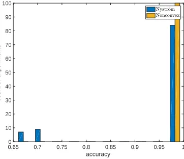
Both Nystr¨om method and our nonconvex optimization (1) give approximation in the form of M ≈XcXc>, so clustering analysis can be directly implemented based onXc. We
implement k-means on the rows ofXcwith 20 repetitions, and Figure 9 compares the two
methods in the distribution of clustering accuracies. It clearly shows that our nonconvex optimization (1) yields accurate clustering throughout the 100 tests while the Nystr¨om method results in poor clustering occasionally.
Moreover, during the iterations of the nonconvex method, the regularization term never activate throughout the 100 simulations. Therefore, empirically speaking, the performances of our numerical tests will remain the same if we simply set λ= 0.
4. Proofs
0.23 0.24 0.25 0.26 0.27 0.28 0.29 relative error
0 10 20 30 40 50 60 70 80 90 100
count of experiments
(a) Relative error kMapprox−M2kF kM2kF .
0.04 0.06 0.08 0.1 0.12 0.14 0.16 0.18 0.2 0.22 relative error
0 10 20 30 40 50 60 70 80 90 100
count of experiments
(b) Relative error kMapprox−MkF kMkF .
Figure 8: Relative errors for Nystr¨om method with sampling ratepNys≈0.01 and nonconvex method with sampling rate pNCVX=
pNys 2.5 .
0.65 0.7 0.75 0.8 0.85 0.9 0.95 1 accuracy
0 10 20 30 40 50 60 70 80 90 100
count of experiments
Figure 9: Clustering accuracy for Nystr¨om method with sampling rate pNys ≈ 0.01 and nonconvex method with sampling rate pNCVX= pNys2.5 .
4.1. Supporting lemmas
In this section, we give some useful supporting lemmas. The following lemma is well known in the literature, see, e.g.,Vu (2018) andBandeira et al. (2016).
Lemma 4 There is a constant Cv > 0 such that the following holds. If Ω is sampled
according to the off-diagonal symmetric Ber(p) model, then
P h
kΩ−pJk>Cv
p
np(1−p) +Cv
p
logn
i
6n−3.
Definition 5 (Cand`es and Recht 2009) For any subspace U of Rn of dimension r,
de-notePU :Rn→Rn as the orthogonal projection onto U. Define
µ(U) := n
r 1max6i6nkPUeik 2
2, (9)
where e1, . . . ,en represents the standard orthogonal basis of Rn.
As with Theorem 4.1 in Cand`es and Recht (2009), for the off-diagonal symmetric Ber(p) model, we also have:
Lemma 6 Let Ωbe sampled according to the off-diagonal symmetric Ber(p) model. Define
T :={M ∈Rn×n|(I−PU)M(I−PU) =0, M symmetric},
where U is a fixed subspace of Rn. Let PT be the Euclidean projection on to T: For any
symmetric matrix M ∈Rn×n,
PT(M) =PUM+M PU−PUM PU.
Then there is an absolute constant Cc, such that for any δ∈(0,1], if p>Ccµ(U) dim(δ2nU) logn
with µ(U) defined in (9), in an event Ec with probabilityP[Ec]>1−n−3, we have
p−1kPTPΩPT −pPTk6δ.
InGross(2011) andGross and Nesme(2010), similar results are given for symmetric uniform sampling with/without replacement. The proof of Lemma6is very similar to that inRecht (2011).
The first and second order optimality conditions of f(X) satisfy the following properties:
Lemma 7 (Ge et al. 2016, Proposition 4.1) The first order optimality condition of
ob-jective function (1) is
∇f(X) = 2PΩ(XX>−M)X +λ∇Gα(X) =0,
and the second order optimality condition requires that for any H ∈Rn×r, we have
vec(H)>∇2f(X) vec(H)
=kPΩ(HX>+XH>)kF2 + 2hPΩ(XX>−M),PΩ(HH>)i+λvec(H)>∇2Gα(X) vec(H) >0.
In the sequel, we are going to present our key lemma which will be used multiple times throughout this section. For any matrix M1,M2 ∈ Rn1×n2, any set Ω0 ∈ [n1]×[n2] and any real numbert∈R, we introduce following notation for simplicity of notations:
Lemma 8 LetΩ0be any index set in[n1]×[n2], andΩ0∈Rn1×n2 be defined correspondingly
as in Section 2.1. For any A ∈ Rn1×r1,B ∈ Rn1×r2,C ∈ Rn2×r1,D ∈ Rn2×r2, and any
t∈R, there holds
|DΩ0,t(AC>,BD>)|6kΩ0−tJk
v u u t
n1
X
k=1
kAk,·k22kBk,·k22 v u u t
n2
X
k=1
kCk,·k22kDk,·k22. (11)
We will use this result for Ω0 = Ω, t=pfor multiple times later. Note that here we do not make any assumptions on Ω0 and this is a deterministic result. The proof of this lemma is deferred to Section4.3.1. This result extends the following lemma given inBhojanapalli and Jain (2014) andLi et al.(2016b):
Lemma 9 (Bhojanapalli and Jain 2014; Li et al. 2016b) Suppose matrixM ∈Rn1×n2
can be decomposed asM =BD>, letΩ0 ⊂[n1]×[n2]be any index set. Then for anyt∈R,
we have
kPΩ0(M)−tMk6kΩ0−tJkkBk2,∞kDk2,∞.
Lemma8is applied in our proof of Lemma12in replace of Theorem D.1 inGe et al.(2016) to derive tighter control of perturbation terms, i.e.,K2(X), K3(X) and K4(X) defined in (14). Their result is given here for the purpose of comparison.
Lemma 10 (Ge et al. 2016, Theorem D.1) With high probability over the choice ofΩ,
for any two rank-r matrices W,Z ∈Rn×n, we have
|hPΩ(W),PΩ(Z)i −phW,Zi|
6OkWk`∞kZk`∞nrlogn+ppnrkWk`∞kZk`∞kWkFkZkF logn.
InSun and Luo(2016),Chen and Wainwright(2015) andZheng and Lafferty(2016), upper bounds are given to kPΩ(HH>)k2
F for any H. To be more precise, they assume Ω is sampled according to the i.i.d. Bernoulli model with probability p. If p >Clognn for some sufficient large absolute constantC, there holds
kPΩ(HH>)k2
F −pkHk4F 6C √
np n
X
i=1
kHi,·k42 (12)
with high probability. In contrast, by combining Lemma4 and Lemma8, there holds
|kPΩ(HH>)k2
F −pkHH>k2F|6C √
np n
X
i=1
kHi,·k42 (13)
with high probability. This is tighter than (12) in that kHH>kF 6 kHk2
F. Moreover, comparing to (12), our result (13) directly measures the difference between kPΩ(HH>)k2
F and its expectation pkHH>k2
4.2. A proof of Theorem 2
This section aims to prove Theorem 2. The proof is basically divided into two parts: In Section 4.2.1, we discuss the landscape of objective function f(X) and then define the auxiliary functionK(X). We show that the span of local minima off(X) can be controlled by the superlevel set ofK(X): {X ∈Rn×r|K(X)>0}. In Section4.2.2, we give a uniform upper bound ofK(X) in order to control the above superlevel set.
4.2.1. Landscape of objective function f and auxiliary function K
Denote Ur := [ √
σ1u1 . . . √
σrur]. For a given X ∈ Rn×r, suppose that X>Ur has SVD
X>Ur =ADB>, and letRX,Ur :=BA
>∈O(r) andU :=U
rRX,Ur, whereO(r) denotes the set ofr×rorthogonal matrices{R∈Rr×r|R>R=RR>=I}. ThenX>U =ADA>
is a positive semidefinite matrix. Then also holds UrUr>=U U>.
Denote ∆ := X −U, and define the following auxiliary function introduced in Jin et al. (2017) and Ge et al.(2017):
K(X) := vec(∆)>∇2f(X) vec(∆)−4h∇f(X),∆i.
The first and second order optimality conditions for any local minimum Xc imply that
K(Xc)>0. In other words, we have
{All local minima off(X)} ⊂ {X ∈Rn×r|K(X)>0}.
To study the properties of the local minima of f(X), we can consider the superlevel set of K(X): {X ∈Rn×r |K(X) >0} instead. In order to get a clear representation ofK(X),
one can plug in the formulas of gradient and Hessian in Lemma 7. By repacking terms in Ge et al. (2017, Lemma 7), and given hU∆>,Ni = 0, due to the definition of U and N, K(X) can be decomposed as follows:
Lemma 11 (Ge et al. 2017, Lemma 7) Uniformly for all X ∈Rn×r, as well as
corre-sponding U and∆ defined above, we have
K(X) =pk∆∆>kF2 −3kXX>−U U>k2F
| {z }
K1(X)
+DΩ,p(∆∆>,∆∆>)−3DΩ,p(XX>−U U>,XX>−U U>)
| {z }
K2(X) +λ
vec(∆)>∇2Gα(X) vec(∆)−4h∇Gα(X),∆i
| {z }
K3(X)
+ 6DΩ,p(∆∆>,N) + 8DΩ,p(U∆>,N) + 6ph∆∆>,Ni
| {z }
K4(X)
,
(14)
Notice that in Theorem 2, we are only concerned about the difference between XX> and
Mr(orM), which remains the same by replacingX withXf=XR, for anyR∈O(r). On
the other hand, by the definition ofRX,Ur, we haveRXR,Ur =RX,UrRfor any R∈O(r), which impliesUe =U R and ∆e =∆R. Now we have
f
XXf>=XX>,UeUe>=U U>,∆e∆e>=∆∆>,Ue∆e>=U∆>,
which meansKi(Xf) =Ki(X) fori= 1,2,4. As forK3, byGe et al.(2017, Lemma 18), we
have
vec(∆)>∇2Gα(X) vec(∆)−4h∇Gα(X),∆i =4
n
X
i=1
[(kXi,·k2−α)+]3
kXi,·k22k∆i,·k22− hXi,·,∆i,·i2
kXi,·k32
+ 12 n
X
i=1
[(kXi,·k2−α)+]2
hXi,·,∆i,·i2
kXi,·k22
−16 n
X
i=1
[(kXi,·k2−α)+]3
hXi,·,∆i,·i
kXi,·k2 .
SinceR∈O(r), we havekXfi,·k2=kXi,·k2,k∆ei,·k2 =k∆i,·k2 andhXfi,·,∆ei,·i=hXi,·,∆i,·i,
so we have K3(Xf) =K3(X). Putting things together, we have K(Xf) =K(X).
Therefore, if we want to show that any X with K(X) >0 satisfies (4) and (5) with high probability, without loss of generality, we can assume that X satisfies the property that
X>Ur is a positive semidefinite matrix, i.e.,U =Ur.
4.2.2. Proof of Theorem 2.
In order to prove our main result, we first give a uniform upper bound ofK(X). Then for any local minimumXc,K(Xc)>0, the property enables us to solve for the range of possible
c
X. For simplicity of notations, denoteνr :=kMrk`∞.
Lemma 12 Assume that tuning parameters α, λ satisfy 100√νr 6α 6200
√
νr,100kΩ− pJk 6 λ6 200kΩ−pJk, and p > CSlognn with some absolute constant CS. Then, in an
event E with probability P[E]> 1−2n−3, uniformly for all X ∈Rn×r and corresponding
∆ defined as before, we have
4
X
i=2
Ki(X)610−3p
h
k∆>∆k2F +kU∆>k2Fi
+C3p r
X
i=1
(
C4
rn
p + logn
p
νr+C4σ2r+1−i−σi
+
)2
+C3
[p(1−p)n+ logn]rkNk2 `∞
p .
(15)
Recall by the way we define ∆,
kXX>−U U>k2F =kU∆>+∆U>+∆∆>k2F
=k∆∆>k2F + 2k∆U>k2F + 2h∆U>,U∆>i+ 4h∆∆>,U∆>i. (16) By the definition of matrix inner product, we have
kU∆>k2F =hU∆>,U∆>i= trace(∆U>U∆>) = trace(U>U∆>∆)
=hU>U,∆>∆i, (17) and
h∆∆>,U∆>i= trace(∆∆>U∆>) = trace(∆>∆∆>U) =h∆>∆,∆>Ui. (18) Here we use the fact that trace(AB) = trace(BA) for any matrix A and B with suitable size. Moreover, since we choose U such that U>X is positive semidefinite, U>∆=∆>U
and U>(∆+U)0. Therefore, we also have
h∆U>,U∆>i= trace(U∆>U∆>) = trace(∆U>∆U>) = trace(U>∆U>∆)
=h∆>U,U>∆i=h∆>U,∆>Ui=k∆>Uk2F (19) and
h∆>∆,U>U+∆>Ui=h∆>∆,(U +∆)>Ui>0. (20) Here (20) also uses the fact that inner product of two positive semidefinite matrices is non-negative.
Now denotea:=k∆>∆kF =k∆∆>kF, b:=k∆>UkF and
ψ:=C3
r
X
i=1
(
C4
rn
p + logn
p
νr+C4σ2r+1−i−σi
+
)2
+ [p(1−p)n+ logn]rkNk 2 `∞
p2
.
Putting Lemma 11and Lemma 12 together, and using (16), we have
K(X)
p 61.001k∆∆
>k2
F −3kXX>−U U>k2F + 10−3kU∆>k2F +ψ =1.001a2−3
h
k∆∆>k2F + 2k∆U>k2F + 2h∆U>,U∆>i+ 4h∆∆>,U∆>ii + 10−3kU∆>k2F +ψ,
(21)
By putting (17), (18), (19), (21) together,
K(X)
p 61.001a
2−3k∆∆>k2
F −6k∆U>k2F −6h∆U>,U∆>i −12h∆∆>,U∆>i + 10−3kU∆>k2F +ψ
=−1.999a2−6hU>U,∆>∆i −6k∆>Uk2F −12h∆>∆,∆>Ui + 10−3hU>U,∆>∆i+ψ
=−1.999a2− h∆>∆,5.999U>U + 12∆>Ui −6b2+ψ.
Therefore, combining with (20),
K(X)
p 6−1.999a
2−6.001h∆>
∆,∆>Ui −6b2+ψ
6−1.999a2+ 6.001ab−6b2+ψ
(23)
holds for allX ∈Rn×r. For the last line, we apply Cauchy-Schwarz inequality for matrices,
i.e.,
|h∆>∆,∆>Ui|6k∆>∆kFk∆>UkF.
Note that for any local minimum Xc, we have K(Xc) > 0. Replacing X with Xcin (23),
there holds
−1.999a2+ 6.001ab−6b2+ψ>0, which further implies
06a6C5
p
ψ, 06b6C5
p
ψ. (24)
From (22), we have
K(Xc)
p 6−1.999a
2− h∆>∆,5.999U>U+ 12∆>Ui −6b2+ψ.
Recall from (17), kU∆>k2 F =hU
>U,∆>∆i, and K( c
X) > 0. Therefore, combining with (24),
5.999kU∆>k2F 6−1.999a2− h∆>∆,12∆>Ui −6b2+ψ 6−1.999a2+ 12k∆>∆kFk∆>UkF −6b2+ψ 6−1.999a2+ 12ab−6b2+ψ
6C6ψ.
(25)
From (21),
K(Xc)
p 61.001k∆∆
>k2
F −3kXcXc>−U U>kF2 + 10−3kU∆>k2F +ψ.
Using the fact that K(Xc)>0 again, we have
3kXcXc>−U U>k2F 61.001k∆∆>k2F + 10−3kU∆>k2F +ψ
Combining with (24), (25), we futher have
3kXcXc>−U U>k2F 61.001a2+C7ψ+ψ6C8ψ. (26)
Therefore, (4) is directly implied by (26). Notice that
kXcXc>−Mk2F =kXcXc>−U U>k2F−2hXcXc>,Ni+kNk2F 6kXcXc>−U U>k2F+kNk2F
4.3. Proofs of supporting lemmas
We present in this section the proofs of lemmas stated in previous sections.
4.3.1. A proof of Lemma 8
Proof First of all, by using the definition of matrix inner product and Hadamard product,
we have
|hPΩ0(AC>),PΩ0(BD>)i −thAC>,BD>i|=|hΩ0−tJ,(AC>◦BD>)i| 6kΩ0−tJkk(AC>◦BD>)k∗,
(27)
The inequality holds by matrix H¨older’s inequality. So the only thing left over is to give a bound of k(AC>◦BD>)k∗. Notice one can decompose the matrix into sum of rank one
matrices as following
AC>◦BD>=
r1
X
k=1
A·,kC·>,k
!
◦ r2
X
k=1
B·,kD>·,k
! = r1 X l=1 r2 X m=1
(A·,l◦B·,m)(C·,l◦D·,m)>.
RecallM·,j= (M1,j, M2,j, . . . , Mn,j)> denotes the j-th column of any matrix M ∈Rn×m.
Therefore, one can upper bound the nuclear norm via
k(AC>◦BD>)k∗ 6
r1 X l=1 r2 X m=1
k(A·,l◦B·,m)(C·,l◦D·,m)>k∗
= r1 X l=1 r2 X m=1
kA·,l◦B·,mk2kC·,l◦D·,mk2
= r1 X l=1 r2 X m=1 v u u t n1 X k=1 A2
k,lB2k,m
v u u t n2 X k=1 C2
k,lD2k,m,
where the first line is by the triangle inequality and we can replace nuclear norm by vector `2 norms in second line since the summands are all rank one matrices. By applying the Cauchy-Schwarz inequality for twice, we can obtain
k(AC>◦BD>)k∗6 v u u t r1 X l=1 r2 X m=1 n1 X k=1 A2
k,lBk,m2
v u u t r1 X l=1 r2 X m=1 n2 X k=1 C2
k,lDk,m2
= v u u t n1 X k=1
kAk,·k22kBk,·k22 v u u t n2 X k=1
kCk,·k22kDk,·k22.
(28)
Combining (27) and (28) together, we have
|hPΩ0(AC>),PΩ0(BD>)i −thAC>,BD>i| 6kΩ0−tJk
v u u t n1 X k=1
kAk,·k22kBk,·k22 v u u t n2 X k=1
4.3.2. A proof of Lemma 12
Proof The proof of Lemma 12 can be divided into the controls of K2(X), K3(X) and
K4(X) separately. ForK2(X), we have
Lemma 13 In an event Ea with probabilityP[Ea]>1−n−3, uniformly for allX ∈Rn×r
and corresponding ∆ defined as before, we have
K2(X)6kΩ−pJk
"
19 n
X
i=1
k∆i,·k42+ 18νrk∆k2F + 9νr r
X
i=s+1 σi
#
+ 3×10⁻⁴pkU∆>k2F,
where s is defined by
s:= max
s6r, σs>Cp
νrlogn p
(29)
with Cp an absolute constant. Set s= 0 if σ1 < Cpνrlogp n.
ForK3(X), we use a modified version of Ge et al.(2017, Lemma 11):
Lemma 14 (Ge et al. 2017, Lemma 11) If α > 100√νr, then uniformly for all X ∈
Rn×r and corresponding ∆ defined as before, we have
K3(X)6199.54λα2k∆k2F −0.3λ n
X
i=1
k∆i,·k42.
The main modification we have made is that we keep the extra negative term. We will give a proof in the appendix for completeness.
ForK4(X), we have
Lemma 15 Uniformly for allX ∈Rn×r and corresponding ∆ defined as before, we have
K4(X)65×10−4pk∆∆>kF2 + 2×10⁻⁴pkU∆>k2F +C10
rkPΩ(N)−pNk2 p
+ 6ph∆∆>,Ni.
We can apply Lemma 4 together with Lemma9 to bound kPΩ(N)−pNk and kΩ−pJk (similar result can also be found in Keshavan et al. (2010b)): As long as p>CSlognn with some absolute constant CS, there is an absolute constant C9, such that
kPΩ(N)−pNk6C9
p
np(1−p) +C9
p
logn
and
kΩ−pJk6C9 √
np (31)
hold in an eventEb with probability P[Eb]>1−n−3.
By putting Lemma13, Lemma14 and Lemma15 together, we have
4
X
i=2
Ki(X)6kΩ−pJk
"
19 n
X
i=1
k∆i,·k42+ 18νrk∆k2F + 9νr r
X
i=s+1 σi
#
+ 3×10⁻⁴pkU∆>k2F
+ 199.54λα2k∆k2F −0.3λ n
X
i=1
k∆i,·k42+ 5×10
−4pk∆∆>k2 F
+ 2×10⁻⁴pkU∆>k2F +C10
rkPΩ(N)−pNk2
p + 6ph∆∆
>
,Ni.
Replacingα, λby the assumption 100√νr 6α6200 √
νr,100kΩ−pJk6λ6200kΩ−pJk, we futher have
4
X
i=2
Ki(X)6kΩ−pJk
"
19 n
X
i=1
k∆i,·k42+ 18νrk∆k2F + 9νr r
X
i=s+1 σi
#
+ 3×10⁻⁴pkU∆>k2F
+ 7.9816×10⁸νrkΩ−pJkk∆k2F −30kΩ−pJk n
X
i=1
k∆i,·k42+ 5×10⁻⁴pk∆∆>k2F
+ 2×10⁻⁴pkU∆>k2 F +C10
rkPΩ(N)−pNk2
p + 6ph∆∆
>,Ni.
Combining with (30) and (31), and applying union bound,
4
X
i=2
Ki(X)6(19−30)kΩ−pJk n
X
i=1
k∆i,·k42+ (18 + 7.9816×10⁸)νrkΩ−pJkk∆k2F
+ 9νrkΩ−pJk r
X
i=s+1
σi+ (3 + 2)×10−4pkU∆>k2F
+ 5×10⁻⁴pk∆∆>k2F +C10
rkPΩ(N)−pNk2
p + 6ph∆∆
>
,Ni
65×10−4phk∆>∆k2
F +kU∆>k2F
i
+C3
p(1−p)n+ logn p rkNk
2 `∞
+C11 √
npνrk∆k2F +C12 √
npνr r
X
i=s+1
σi+ 6ph∆∆>,Ni,
(32)
holds in an event E with probability P[E]>1−2n−3.
Fork∆>∆k2
F, we have
k∆>∆k2F =h∆>∆,∆>∆i= r
X
i=1
whereσi(∆) denotesi-th largest singular value of ∆.
In order to proceed, we need the following von Neumann’s trace inequality:
Lemma 16 (Bhatia 2013, Problem III.6.14) Let A,B∈Rn×n be two symmetric
ma-trices, λ1(A) >λ2(A) >· · ·>λn(A) and λ1(B)> λ2(B)>· · · >λn(B) are eigenvalues of A and B. Then the following holds:
n
X
i=1
λi(A)λn+1−i(B)6hA,Bi6 n
X
i=1
λi(A)λi(B).
This result can also be derived from Schur-Horn theorem (see, e.g., Marshall et al. (2011, Theorem 9.B.1, Theorem 9.B.2)) together with Abel’s summation formula.
From Lemma16, we have
kU∆>k2F = trace(∆U>U∆>) =hU>U,∆>∆i >
r
X
i=1
λr+1−i(U>U)λi(∆>∆) = r
X
i=1
σi2(∆)σ2r+1−i(U), (34)
and
h∆∆>,Ni6 n
X
i=1
λi(∆∆>)λi(N) = r
X
i=1
σi2(∆)σi(N). (35)
Here we use the fact thatλi(U>U) =σi2(U),λi(∆>∆) =σ2i(∆),λi(N) =σi(N) and
λi(∆∆>) =
σ2i(∆) i= 1,· · · , r 0 i=r+ 1,· · · , n.
Putting (33), (34) and (35) together we have
−5×10⁻⁴phk∆>∆k2
F +kU∆>k2F
i
+C11 √
npνrk∆k2F + 6ph∆∆>,Ni 6−5×10⁻⁴p
" r X
i=1
σi4(∆) + r
X
i=1
σ2i(∆)σr+12 −i(U)
#
+C11 √
npνr r
X
i=1 σi2(∆)
+ 6p r
X
i=1
σi2(∆)σi(N)
65×10−4p r
X
i=1
−σi4(∆) +
C13
rn
pνr−σ 2
r+1−i(U) +C13σi(N)
σ2i(∆)
.
is taken over ˆx= 12[b]+, and the maximum value is 14{[b]+}2. Therefore, we have −5×10⁻⁴p
h
k∆>∆k2F +kU∆>k2Fi+C11 √
npνrk∆k2F + 6ph∆∆
>
,Ni
6C14p r X i=1 ( C13 r n pνr−σ
2
r+1−i(U) +C13σi(N)
+
)2
=C14p r X j=1 ( C13 r n pνr−σ
2
j(U) +C13σr+1−j(N)
+
)2
=C14p r X j=1 ( C13 r n
pνr+C13σ2r+1−j−σj
+
)2
.
(36)
In the second last line, we let j=r+ 1−i. In the last line, we use the fact that
σr+1−j(N) =σr+r+1−j(M) =σ2r+1−j and
σ2j(U) =σj(U U>) =σj(Mr) =σj(M) =σj. Finally putting (32) and (36) together we have
4
X
i=2
Ki(X)610×10−4p
h
k∆>∆k2F +kU∆>k2Fi+C3
p(1−p)n+ logn p rkNk
2 `∞
−5×10⁻⁴p
h
k∆>∆k2F +kU∆>k2Fi+C11 √
npνrk∆k2F +C12
√ npνr
r
X
i=s+1
σi+ 6ph∆∆>,Ni
610−3phk∆>∆k2
F +kU∆>k2F
i
+C3
p(1−p)n+ logn p rkNk
2 `∞
+C14p r X i=1 ( C13 rn
pνr+C13σ2r+1−i−σi
+
)2
+C12 √
npνr r
X
i=s+1 σi.
(37)
Recall by the definition ofsin (29), for anyi > s, we haveσi< Cpνrlogp n. By choosingC13 sufficient large, i.e.,C13>2Cp, we have
C13 rn p + logn p
νr+C13σ2r+1−i−σi >C13
rn
p + logn
p
νr−2σi+σi
>C13
rn
p + logn
p
νr−2Cp
νrlogn p +σi
=C13
r
n
pνr+σi+ (C13−2Cp)
νrlogn p
>C13
r
n
Therefore, for alli > s, ( C13 rn p + logn p
νr+C13σ2r+1−i−σi
+ )2 > C13 rn
pνr+σi
2
>
rn
pνrσi.
Combining with (37), we have
4
X
i=2
Ki(X)610−3p
h
k∆>∆k2F +kU∆>k2Fi
+C14p r X i=1 ( C13 rn p + logn p
νr+C13σ2r+1−i−σi
+
)2
+C12p r X i=s+1 ( C13 rn p + logn p
νr+C13σ2r+1−i−σi
+
)2
+C3
p(1−p)n+ logn p rkNk
2 `∞
610−3phk∆>∆k2
F +kU∆
>k2 F
i
+C3p r X i=1 ( C4 r n p + logn p
νr+C4σ2r+1−i−σi
+
)2
+C3
p(1−p)n+ logn p rkNk
2 `∞
which finishes the proof.
4.3.3. A proof of Lemma 13
Proof Recall that we define ∆as∆:=X−U,DΩ,p(XX>−U U>,XX>−U U>) can
be decomposed as following
DΩ,p(XX>−U U>,XX>−U U>)
=DΩ,p(U∆>+∆U>+∆∆>,U∆>+∆U>+∆∆>) =DΩ,p(U∆>+∆U>,U∆>+∆U>)
| {z }
1
+DΩ,p(∆∆>,∆∆>)
| {z }
2
+ 4DΩ,p(U∆>,∆∆>)
| {z }
3
. (38)
First for 2 and 3 , by applying Lemma 8,
| 2 |=|DΩ,p(∆∆>,∆∆>)|6kΩ−pJk n
X
i=1
k∆i,·k42 (39)
and
| 3 |= 4|DΩ,p(U∆>,∆∆>)|64kΩ−pJk
v u u t n X i=1
kUi,·k22k∆i,·k22 v u u t n X i=1
k∆i,·k42
62kΩ−pJkνrk∆k2F + 2kΩ−pJk n
X
i=1
k∆i,·k42,
(40)
where for the second inequality we use the fact that 2xy6x2+y2.
Finally for 1 , if U is good enough such that the incoherence µ(U) is well-bounded, then we can apply Lemma 6 directly and get a tight bound. If µ(U) is not good enough, we want to split U into two parts and hope first few columns have good incoherence. To be more precise, recall that we assume U =Ur = [
√
σ1u1 . . . √
σrur], similar to (8), for the incoherence of the first kcolumns, we have
µ(colspan([√σ1u1 . . . √
σkuk]))
=n kmaxi
k
X
j=1
u2i,j 6 n kσk max i k X j=1
σju2i,j 6 n kσk max i r X j=1
σju2i,j 6 nνr kσk
, (41)
whereµ(·) is defined in (9).
For fixed s defined as in (29), denote first s columns of U as U1, and remaining part as
U2. Decompose U as U = [U1 U2], and ∆ can also be decomposed as ∆ = [∆1 ∆2] correspondingly. Note by our assumption thatU =Ur, we have (U1)>U2 =0. So we can further decompose the first term of (38) as
1 =DΩ,p(U∆>+∆U>,U∆>+∆U>) =DΩ,p
[U1 U2][∆1 ∆2]>+ [∆1 ∆2][U1U2]>,[U1 U2][∆1 ∆2]> +[∆1∆2][U1 U2]>
=DΩ,p
U1(∆1)>+∆1(U1)>,U1(∆1)>+∆1(U1)>
| {z }
A1
+ 4DΩ,p
U1(∆1)>,U2(∆2)>
| {z }
A2
+ 2DΩ,p
U2(∆2)>,U2(∆2)>
| {z }
A3
+ 2DΩ,p
U2(∆2)>,∆2(U2)>
| {z }
A4
+ 4DΩ,p
U1(∆1)>,∆2(U2)>
| {z }
A5
.
Now we can apply tight approximation Lemma 6to the first term of (42). By the way we choose s, combining with (41),
p>Cp
νrlogn σs >
Cp
νrlogn σs
·µ colspan(U 1)
sσs nνr
=Cp
µ colspan(U1)
slogn
n .
By choosingCp sufficient large, Lemma 6 ensures that
|A1|=
DΩ,p
U1(∆1)>+∆1(U1)>,U1(∆1)>+∆1(U1)>
62.5×10⁻⁵pkU1(∆1)>+∆1(U1)>k2F 65×10−5p(kU1(∆1)>k2F +k∆1(U1)>k2F) 610−4pkU∆>k2
F
(43)
hold in an eventEawith probability P[Ea]>1−n−3, where the second inequality uses the
fact that (x+y)2 62x2+ 2y2, and last inequality uses the fact that (U1)>U2=0. For the rest terms in (42), by applying Lemma8 we have
|A2|=4|DΩ,p(U1(∆1)>,U2(∆2)>)| 64kΩ−pJk
v u u t n X i=1 kU1
i,·k22kUi,2·k22
v u u t n X i=1 k∆1
i,·k22k∆2i,·k22
62kΩ−pJk
"
νrkU2k2F + n
X
i=1
k∆i,·k42
#
(44)
for the second term in (42), where the second inequality use the fact thatkU1
i,·k22 6kUi,·k226
νr,k∆1i,·k22 6 k∆i,·k22,k∆2i,·k22 6k∆i,·k22 and 2xy 6x2+y2. For the third term, applying
Lemma8 again we have
|A3|=2|DΩ,p(U2(∆2)>,U2(∆2)>)| 62kΩ−pJk
v u u t n X i=1 kU2
i,·k42
v u u t n X i=1 k∆2
i,·k42
6kΩ−pJk
"
νrkU2k2F + n
X
i=1
k∆i,·k42
#
,
(45)
where for the second inequality we also use the properties used in bounding second term. For the fourth and last term in (42), applying Lemma 8 and properties listed above, we have
|A4|=2|DΩ,p(U2(∆2)>,∆2(U2)>)| 62kΩ−pJk
n
X
i=1
kUi,2·k22k∆2i,·k2262kΩ−pJkνrk∆k2F
and
|A5|=4|DΩ,p(U1(∆1)>,∆2(U2)>)|
64kΩ−pJk
v u u t
n
X
i=1
kUi,1·k2
2k∆2i,·k22
v u u t
n
X
i=1
kUi,2·k2
2k∆1i,·k22 62kΩ−pJkνrk∆1kF2 + 2kΩ−pJkνrk∆2k2F
=2kΩ−pJkνrk∆k2F.
(47)
Now putting estimations of terms in (42) listed above together, i.e., (43), (44), (45), (46) and (47), we have
| 1 |=|DΩ,p(U∆>+∆U>,U∆>+∆U>)| 6|A1|+|A2|+|A3|+|A4|+|A5| 610−4pkU∆>k2F + 2kΩ−pJk
"
νrkU2k2F + n
X
i=1
k∆i,·k42
#
+kΩ−pJk
"
νrkU2k2F + n
X
i=1
k∆i,·k42
#
+ 2kΩ−pJkνrk∆k2F + 2kΩ−pJkνrk∆k2F
6kΩ−pJk
"
3νrkU2k2F + 3 n
X
i=1
k∆ik42+ 4νrk∆k2F
#
+ 10−4pkU∆>k2 F.
(48)
Plugging estimations (39), (40) and (48) back to (38), we have
|DΩ,p(XX>−U U>,XX>−U U>)| 6| 1 |+| 2 |+| 3 |
6kΩ−pJk
"
3νrkU2k2F + 3 n
X
i=1
k∆ik42+ 4νrk∆k2F
#
+ 10−4pkU∆>k2F
+kΩ−pJk n
X
i=1
k∆i,·k42+ 2kΩ−pJkνrk∆k2F + 2kΩ−pJk n
X
i=1
k∆i,·k42
=kΩ−pJk
"
3νrkU2k2F + 6 n
X
i=1
k∆ik42+ 6νrk∆k2F
#
Therefore, combining with (39), we have
K2(X)6|DΩ,p(∆∆>,∆∆>)|+ 3|DΩ,p(XX>−U U>,XX>−U U>)| 6kΩ−pJk
n
X
i=1
k∆i,·k42+ 3kΩ−pJk
"
3νrkU2k2F + 6 n
X
i=1
k∆ik42+ 6νrk∆k2F
#
+ 3×10⁻⁴pkU∆>k2F 6kΩ−pJk
"
19 n
X
i=1
k∆ik42+ 18νrk∆k2F + 9νr r
X
i=s+1 σi
#
+ 3×10⁻⁴pkU∆>k2F.
The last line uses the fact thatkU2k2 F =
Pr
i=s+1σi.
4.3.4. A proof of Lemma 15
Proof First, by matrix H¨older’s inequality,
6|h∆∆>,PΩ(N)−pNi|66 √
pk∆∆>k∗
√ r
√
rkPΩ(N)−pNk √
p .
Since ∆∆> is at most rank-r,k∆∆>k∗6
√
rk∆∆>kF. Therefore,
6|h∆∆>,PΩ(N)−pNi|66√pk∆∆>kF √
rkPΩ(N)−pNk √
p
65×10−4pk∆∆>k2F +C15
rkPΩ(N)−pNk2
p .
For the last inequality, we also use the fact that 2xy 6 wx2+ y2
w for all w > 0. Use the same argument we also have
8|hU∆>,PΩ(N)−pNi|62×10−4pkU∆>k2F +C15
rkPΩ(N)−pNk2
p ,
Therefore, by the way we defineK4(X) in (14), we have
K4(X)6|6h∆∆>,PΩ(N)i −6ph∆∆>,Ni|+|8hU∆>,PΩ(N)i −8phU∆>,Ni| + 6ph∆∆>,Ni
65×10−4pk∆∆>k2F + 2×10⁻⁴pkU∆>k2F +C10
rkPΩ(N)−pNk2 p
5. Discussions
This paper studies low-rank approximation of a positive semidefinite matrix from partial entries via nonconvex optimization. We established a model-free theory for local-minimum based low-rank approximation without any assumptions on its rank, condition number or eigenspace incoherence parameter. We have also improved the state-of-the-art sampling rate results for nonconvex matrix completion with no spurious local minima in Ge et al.(2016, 2017), and have investigated the performance of the proposed nonconvex optimization in presence of large condition numbers, large incoherence parameters, or rank mismatching. The nonconvex optimization is further applied to the problem of memory-efficient kernel PCA. Compared to the well-known Nystr¨om methods, numerical experiments illustrate that the proposed nonconvex optimization approach yields more stable results in both low-rank approximation and clustering.
For future research, we are interested in understanding whether and how fast first-order methods converge to a neighborhood of the set of local minima with theoretical guarantees. In fact, a series of recent works in nonconvex optimization have discussed why and when first-order iterative algorithms can avoid strict saddle points almost surely. For example, in a very recent work by Lee et al.(2017), the authors show that under mild conditions of the nonconvex objective function, a variety of first order algorithms can avoid strict saddle points with almost all initialization, which extends the previous results inLee et al. (2016) and Panageas and Piliouras (2017). We are particularly interested in the robust version of the strict saddle points condition discussed in Ge et al. (2015) and Jin et al. (2017), referred to as (θ, γ, ζ)-strict saddle, under which noisy stochastic/deterministic gradient descent methods are proven to converge to a neighborhood of the local minima. In fact, Ge et al. (2017, Theorem 12) shows that the nonconvex optimization (1) satisfies certain (θ, γ, ζ)-strict saddle conditions as long asM is exactly of rankr, its condition number and eigenspace incoherence parameter are well-bounded, and the sampling rate is sufficiently large, but their argument cannot be straightforwardly extended to the model-free settings. We plan to explore the (θ, γ, ζ)-strict saddle conditions for (1) under a model-free framework in future.
Acknowledgments
We would like to acknowledge Taisong Jing for pointing us to the reference Bhatia(2013).
References
Dimitris Achlioptas and Frank McSherry. Fast computation of low-rank matrix approxima-tions. Journal of the ACM (JACM), 54(2):9, 2007.
Dimitris Achlioptas, Frank McSherry, and Bernhard Sch¨olkopf. Sampling techniques for kernel methods. In Advances in Neural Information Processing Systems, pages 335–342, 2002.