Gaussian Processes with Linear Operator Inequality
Constraints
Christian Agrell [email protected]
Department of Mathematics University of Oslo
P.O. Box 1053 Blindern, Oslo N-0316, Norway
Group Technology and Research DNV GL
P.O. Box 300, 1322 Høvik, Norway
Editor:Andreas Krause
Abstract
This paper presents an approach for constrained Gaussian Process (GP) regression where we assume that a set of linear transformations of the process are bounded. It is motivated by machine learning applications for high-consequence engineering systems, where this kind of information is often made available from phenomenological knowledge. We consider a GP
f over functions onX ⊂Rntaking values in
R, where the processLf is still Gaussian when
L is a linear operator. Our goal is to modelf under the constraint that realizations ofLf
are confined to a convex set of functions. In particular, we require thata≤ Lf ≤b, given two functionsaandbwherea < bpointwise. This formulation provides a consistent way of encoding multiple linear constraints, such as shape-constraints based on e.g. boundedness, monotonicity or convexity. We adopt the approach of using a sufficiently dense set of virtual observation locations where the constraint is required to hold, and derive the exact posterior for a conjugate likelihood. The results needed for stable numerical implementation are derived, together with an efficient sampling scheme for estimating the posterior process. Keywords: Gaussian processes, Linear constraints, Virtual observations, Uncertainty Quantification, Computer code emulation
1. Introduction
Gaussian Processes (GPs) are a flexible tool for Bayesian nonparametric function estima-tion, and widely used for applications that require inference on functions such as regression and classification. A useful property of GPs is that they automatically produce estimates on prediction uncertainty, and it is often possible to encode prior knowledge in a princi-pled manner in the modelling of prior covariance. Some early well-known applications of GPs are within spatial statistics, e.g. meteorology (Thompson, 1956), and in geostatistics (Matheron, 1973) where it is known askriging. More recently, GPs have become a popular choice within probabilistic machine learning (Rasmussen and Williams, 2005; Ghahramani, 2015). Since the GPs can act as interpolators when observations are noiseless, GPs have also become the main approach for uncertainty quantification and analysis involving computer experiments (Sacks et al., 1989; Kennedy and O’Hagan, 2001).
c
Often, the modeler performing function estimation has prior knowledge, or at least hypotheses, on some properties of the function to be estimated. This is typically related to the function shape with respect to some of the input parameters, such as boundedness, monotonicity or convexity. Various methods have been proposed for imposing these types of constraints on GPs (see Section 4.1 for a short review). For engineering and physics based applications, constraints based on integral operators and partial differential equations are also relevant (Jidling et al., 2017; S¨arkk¨a, 2011). What the above constraints have in common is that they are linear operators, and so any combination of such constraints can be written as a single linear operator. For instance, the constraints a1(x) ≤f(x) ≤b1(x),
∂f /∂xi≤0 and ∂2f /∂xj2 ≥0 for some function (or distribution over functions)f :X→Y,
can be written as a(x) ≤ Lf(x)≤b(x) for a(x) = [a1(x),−∞,0], b(x) = [b1(x),0,∞] and L :YX →(YX)3 being the linear operator Lf = [f, ∂f /∂xi, ∂2f /∂x2j].
The motivation for including constraints is usually to improve predictions and to obtain a reduced and more realistic estimate on the uncertainty, the latter having significant impact for risk-based applications. For many real-world systems, information related to constraints in this form is often available from phenomenological knowledge. For engineering systems, this is typically knowledge related to some underlying physical phenomenon. Being able to make use of these constraint in probabilistic modelling is particularly relevant for high-consequence applications, where obtaining realistic uncertainty estimates in subsets of the domain where data is scarce is a challenge. Furthermore, information on whether these types of constraints are likely to hold given a set of observations is also useful for explainability and model falsification. For a broader discussion see (Agrell et al., 2018; Eldevik et al., 2018).
In this paper, we present a model for estimating a function f :Rnx →Rby a constrained GP (CGP) f|D, a(x) ≤ Lf(x)≤b(x). Here Dis a set of observations of (xj, yj), possibly including additive white noise, and f ∼ GP(µ(x), K(x,x0)) is a GP with mean µ(x) and covariance function K(x,x0) that are chosen such that existence of Lf is ensured. Due to the linearity of L, both Lf|D and f|D,Lf remain Gaussian, and our approach is based on modelling f|D,Lf under the constraint a(x)≤ Lf(x)≤b(x). To model the constraint that a(x) ≤ Lf(x) ≤ b(x) for all inputs x, we take the approach of using a finite set of input locations where the constraint is required to hold. That is, we require thata(xv)≤
Lf(xv)≤b(xv) for a finite set of inputs{xv}called the set ofvirtual observation locations. With this approach the CGP is not guaranteed to satisfy the constraint on the entire domain, but a finite set of points {xv} can be found so that the constraint holds globally with sufficiently high probability.
of the covariance matrix of the joint GP may therefore be of concern, both because this scales with the number of observations cubed and because there is typically high serial correlation if there are many virtual observations close together. The general solution is then to restrict the virtual observation set to regions where the probability of occurrence of the constraint is low (Riihimki and Vehtari, 2010; Wang and Berger, 2016). According to Wang and Berger (2016), when they followed this approach in their experiments, they found that only a modest number of virtual observations were typically needed, that these points were usually rather disperse, and the resulting serial correlation was not severe. We draw the same conclusion in our experiments. There is also one benefit with the virtual observation approach, which is that implementation of constraints that only hold on subsets of the domain is straightforward.
For practical use of the model presented in this paper, we also pay special attention to numerical implementation. The computations involving only real observations or only virtual observations are separated, which is convenient when only changes to the constraints are made such as in algorithms for finding a sparse set of virtual observation locations or for testing/validation of constraints. We also provide the algorithms based on Cholesky factorization for stable numerical implementation, and an efficient sampling scheme for estimating the posterior process. These algorithms are based on derivation of the exact posterior of the constrained Gaussian process using a general linear operator, and constitutes the main contribution of this paper.
2. Gaussian Processes and Linear Operators
We are interested in GP regression on functions f :Rnx →Runder the additional inequality constraint a(x) ≤ Lf(x) ≤ b(x) for some specified functions a(x) and b(x), and the class of linear operators {L|Lf : Rnx → Rnc}. Here nx and nc are positive integers, and the subscripts are just used to indicate the relevant underlying space overR. We will make use of the properties of GPs under linear transformations given below.
2.1. Gaussian Process Regression
We consider a Gaussian process f ∼ GP(µ(x), K(x,x0)) given as a prior over functions f :Rnx →R, which is specified by its mean and covariance function
µ(x) =E[f(x)] :Rnx →R,
K(x,x0) =E[(f(x)−µ(x))(f(x0)−µ(x0))] :Rnx×nx →R.
(1)
Let x denote a vector in Rnx and X theN ×nx matrix of N such input vectors. The distribution over the vector f of N latent values corresponding to X is then multivariate Gaussian with
f|X∼ N(µ(X), K(X, X)),
where K(X, X0) denotes the Gram matrixK(X, X0)i,j =K(xi,x0j) for two matrices of input vectors X and X0. Given a set of observations Y = [y1, . . . , yN]T, and under the assumption that the relationship between the latent function values and observed output is Gaussian, Y|f∼ N(f, σ2IN), the predictive distribution for new observations X∗ is still Gaussian with mean and covariance
E[f∗|X∗, X, Y] =µ(X∗) +K(X∗, X)[K(X, X) +σ2IN]−1(Y −µ(X)),
cov(f∗|X∗, X, Y) =K(X∗, X∗)−K(X∗, X)[K(X, X) +σ2IN]−1K(X, X∗).
(2)
Here f∗|X∗ is the predictive distribution of f(X∗) and f∗|X∗, X, Y is the predictive posterior given the dataX, Y. For further details see e.g. Rasmussen and Williams (2005).
2.2. Linear Operations on Gaussian Processes
Let L be a linear operator on realizations of f ∼ GP(µ(x), K(x,x0)). As GPs are closed under linear operators (Rasmussen and Williams, 2005; Papoulis and Pillai, 2002), Lf is still a GP 1. We will assume that the operator produces functions with range in Rnc, but where the input domain Rnx is unchanged. That is, the operator produces functions from
Rnx toRnc. This type of operators on GPs has also been considered by S¨arkk¨a (2011) with applications to stochastic partial differential equations. The mean and covariance ofLf are given by applyingL to the mean and covariance of the argument:
E[Lf(x)] =Lµ(x) :Rnx →Rnc,
cov(Lf(x),Lf(x0)) =LK(x,x0)LT :Rnx×nx →Rnc×nc,
(3)
and the cross-covariance is given as
cov(Lf(x), f(x0)) =LK(x,x0) :Rnx×nx →Rnc, cov(f(x),Lf(x0)) =K(x,x0)LT :Rnx×nx →Rnc.
(4)
The notation LK(x,x0) and K(x,x0)LT is used to indicate when the operator acts on
K(x,x0) as a function of x and x0 respectively. That is, LK(x,x0) = LK(x,·) and
K(x,x0)L = LK(·,x0). With the transpose operator the latter becomes K(x,x0)LT = (LK(·,x0))T. In the following sections we make use of the predictive distribution (2), where observations correspond to the transformed GP underL.
3. Gaussian Processes with Linear Inequality Constraints
Following Section 2.1 and Section 2.2, we let f ∼ GP(µ(x), K(x,x0)) be a GP over real valued functions onRnx, andL a linear operator producing functions fromRnx toRnc. The matrixX and the vectorY will represent N noise perturbed observations: yi =f(xi) +εi withεi i.i.d. N(0, σ2) for i= 1, . . . , N.
We would like to model the posterior GP conditioned on the observationsX, Y, and on the event thata(x)≤ Lf(x)≤b(x) for two functions a(x), b(x) :Rnx →(R∪ {−∞,∞})nc, where ai(x) < bi(x) for all x ∈ Rnx and i= 1, . . . , nc. To achieve this approximately, we start by assuming that the constrainta(x)≤ Lf(x)≤b(x) only holds at a finite set of inputs
xv1, . . . ,xvS that we refer to as virtual observation locations. Later, we will consider how to
specify the set of virtual observation locations such that the constraint holds for anyxwith sufficiently high probability. Furthermore, we will also assume that virtual observations of the transformed process, Lf(xvi), comes with additive white noise with variance σ2
v. We can write this as a(Xv) ≤ Lf(Xv) +εv ≤b(Xv), where Xv = [xv1, . . . ,xvS]T is the matrix containing the virtual observation locations andεv is a multivariate Gaussian with diagonal covariance of elements σ2
v.
We will make use of the following notation: Let Ce(Xv) ∈ RS×nc be the matrix with rows (Ce(Xv))i =Lf(xvi) +εvi for i.i.d. εvi ∼ N(0, σ2vInc), and let C(Xv) denote the event
C(Xv) := ∩S
i=1{a(xvi) ≤ (Ce(Xv))i ≤ b(xvi)}. C(Xv) thus represents the event that the constraint a(x) ≤ Lf(x) +εv ≤ b(x) is satisfied for all points in Xv, and it is defined through the latent variableCe(Xv).
In summary, the process we will consider is stated as
f|X, Y, Xv, C(Xv) :=f|f(X) +ε=Y, a(Xv)≤ Lf(Xv) +εv ≤b(Xv),
where f is a Gaussian process, X, Y is the training data and Xv are the locations where the transformed processLf +εv is bounded. The additive noiseεand εv are multivariate Gaussian with diagonal covariance matrices of elementsσ2 and σv2 respectively.
We also assume that any sub-operator of L is constrained at the same set of virtual locationsXv. This is mainly for notational convenience, and this assumption will be relaxed in Section 3.5. In the following, we let Nv denote the total number of virtual observation locations. Here Nv = S·nc for now, whereas we will later consider Nv =Pni=1c Si where
the i-th sub-operator is associated with Si virtual observation locations.
3.1. Posterior Predictive Distribution
Our goal is to obtain the posterior predictive distributionf∗|X∗, X, Y, Xv, C(Xv). That is: the distribution of f∗ =f(X∗) for some new inputsX∗, conditioned on the observed data
Y =f(X) +εand the constrainta(Xv)≤ Lf(Xv) +εv ≤b(Xv).
To simplify the notation we write f∗|Y, C, excluding the dependency on inputs X, X∗
andXv (as well as any hyperparameter of the mean and covariance function). The posterior predictive distribution is given by marginalizing over the latent variable Ce:
p(f∗, C|Y) =p(f∗|C, Y)p(C|Y),
p(f∗|C, Y) =
Z b(Xv) a(Xv)
p(f∗|C, Ye )p(Ce|Y)dC,e
p(C|Y) =
Z b(Xv) a(Xv)
p(Ce|Y)dC,e
where the limits correspond to the hyper-rectangle in RNv given by the functionsa(·) and
b(·) evaluated at eachxv ∈Xv. The predictive distribution and the probabilityp(C|Y) are given in Lemma 1. p(C|Y) is of interest, as it is the probability that the constraint holds atXv given the dataY.
In the remainder of the paper we will use the shortened notationµ∗=µ(X∗),µ=µ(X),
µv = µ(Xv) and KX,X0 = K(X, X0). For vectors with elements in Rnc, such as Lµv, we
interpret this elementwise. E.g. Lµv(Xv) is given by the column vector [Lµ(xv1)1, . . . ,
Lµ(xv1)nc, . . . ,Lµ(x
v
S)1, . . . ,Lµ(xvS)nc].
We start by deriving the posterior predictive distribution f∗ at some new locations
X∗. The predictive distribution is represented by a Gaussian, f∗|Y, C ∼ N(µ(C),Σ), for some fixed covariance matrix Σ and a mean µ(C) that depends on the random variable
C =Ce|Y, C. The variable Ce = Lf(Xv) +εv remains Gaussian after conditioning on the observations Y, i.e. Ce|Y ∼ N(νc,Σc) with some expectation νc and covariance matrix Σc that can be computed using (3, 4). Applying the constraints represented by the eventC on the random variable Ce|Y just means restricting Ce|Y to lie in the hyper-rectangle defined by the boundsa(Xv) and b(Xv). This means that C=Ce|Y, C is a truncated multivariate Gaussian,C∼ T N(νc,Σc, a(Xv), b(Xv)). The full derivation of the distribution parameters of Cand f∗|Y, C are given in Lemma 1 below, whereas Lemma 2 provides an alternative algorithmic representation suitable for numerical implementation.
Lemma 1 The predictive distributionf∗|Y, C is a compound Gaussian with truncated Gaus-sian mean:
C=Ce|Y, C ∼ T N(Lµv+A1(Y −µ), B1, a(Xv), b(Xv)), (6) where T N(·,·, a, b) is the GaussianN(·,·) conditioned on the hyper-rectangle[a1, b1]× · · · ×
[ak, bk], and
A1 = (LKXv,X)(KX,X+σ2IN)−1, B1=LKXv,XvLT +σ2vINv−A1KX,XvLT,
A2 =KX∗,X(KX,X+σ2IN)−1, B2=KX∗,X∗−A2KX,X∗,
B3=KX∗,XvLT −A2KX,XvLT,
A=B3B1−1, B =A2−AA1, Σ =B2−AB3T.
Moreover, the probability that the unconstrained version of C falls within the constraint region, p(C|Y), is given by
p(C|Y) =p(a(Xv)≤ N(Lµv+A1(Y −µ), B1)≤b(Xv)), (7)
and the unconstrained predictive distribution is
f∗|Y ∼ N(µ∗+A2(Y −µ), B2).
The derivation in Lemma 1 is based on conditioning the multivariate Gaussian (f∗, Y,Ce), and the proof is given in Appendix A. For practical implementation the matrix inversions involved in Lemma 1 may be prone to numerical instability. A numerically stable alternative is given in Lemma 2 below.
In the following lemma, Chol(K) is the lower triangular Cholesky factor of a matrixK. We also let R = (P \Q) denote the solution to the linear system P R =Q for matricesP
andQ, which may be efficiently computed whenP is triangular using forward or backward substitution.
Lemma 2 Let L=Chol(KX,X+σ2IN), v1 =L\KX,XvLT and v2 =L\KX,X∗. Then the matrices in Lemma 1 can be computed as
A1= (LT \v1)T, B1=LKXv,XvLT +σv2IN
v−v
T
1v1,
A2= (LT \v2)T, B2=KX∗,X∗−vT
2v2,
B3=KX∗,XvLT −vT2v1.
Moreover,B1 is symmetric and positive definite. By lettingL1=Chol(B1)andv3=L1\B3T
we also have
A= (LT1 \v3)T, B=A2−AA1, Σ =B2−v3Tv3.
The proof is given in Appendix B. The numerical complexity of the procedures in Lemma 2 is n3/6 for Cholesky factorization of n×n matrices and mn2/2 for solving triangular systems where the unknown matrix isn×m. In the derivation of Lemma 1 and Lemma 2, the order of operations was chosen such that the first Cholesky factorL=Chol(KX,X+σ2IN) only depends onX. This is convenient in the case where the posteriorf∗|Y, C is calculated multiple times for different constraints C or virtual observations Xv, but where the data
3.2. Sampling from the Posterior Distribution
In order to sample from the posterior we can first sample from the constraint distribution (6), and then use these samples in the mean of (5) to create the final samples of f∗|Y, C.
To generate k samples of the posterior at M new input locations, [x∗1, . . . ,x∗M]T =X∗, we use the following procedure
Algorithm 3 Sampling from the posterior distribution
1. Find a matrixQs.t. QTQ= Σ∈RM×M, e.g. by Cholesky or a spectral decomposition.
2. Generate Cek, a Nv ×k matrix where each column is a sample of Ce|Y, C from the distribution in (6).
3. Generate Uk, a M×k matrix with k samples from the standard normalN(0, IM).
4. The M ×k matrix where each column in a sample from f∗|Y, C is then obtained by
[µ∗+B(Y −µ)]⊕col[A(−Lµv⊕colCek) +QUk],
where ⊕col means that the M×1 vector on the left hand side is added to each column of theM ×k matrix on the right hand side.
This procedure is based on the well-known method for sampling from multivariate Gaus-sian distributions, where we have used the property that in the distribution off∗|Y, C, only the mean depends on samples from the constraint distribution.
3.3. Parameter Estimation
To estimate the parameters of the CGP we make use of the marginal maximum likelihood approach (MLE). We define the marginal likelihood function of the CGP as
L(θ) =p(Y, C|θ) =p(Y|θ)p(C|Y, θ), (8)
i.e. as the probability of the dataY and constraintCcombined, given the set of parameters represented byθ. We assume that both the mean and covariance function of the GP prior (1)
µ(x|θ) andK(x,x0|θ) may depend onθ. The log-likelihood, l(θ) = lnp(Y|θ) + lnp(C|Y, θ), is thus given as the sum of the unconstrained log-likelihood, lnp(Y|θ), which is optimized in unconstrained MLE, and lnp(C|Y, θ), which is the probability that the constraint holds atXv given in (7).
In (Bachoc et al., 2018) the authors study the asymptotic distribution of the MLE for shape-constrained GPs, and show that for large sample sizes the effect of including the constraint in the MLE is negligible. But for small or moderate sample sizes the constrained MLE is generally more accurate, so taking the constraint into account is beneficial. However, due to the added numerical complexity in optimizing a function that includes the term lnp(C|Y, θ), it might not be worthwhile. Efficient parameter estimation using the full likelihood (8) is a topic of future research. In the numerical experiments presented in this paper, we therefore make use of the unconstrained MLE. This also makes it possible to compare models with and without constraints in a more straightforward manner.
3.4. Finding the Virtual Observation Locations
For the constraint to be satisfied locally at any input location in some bounded set Ω⊂Rnx
with sufficiently high probability, the set of virtual observation locations Xv has to be sufficiently dense. We will specify a target probability ptarget ∈ [0,1) and find a set Xv,
such that when the constraint is satisfied at all virtual locations inXv, the probability that the constraint is satisfied for anyxin Ω is at leastptarget. The number of virtual observation
locations needed depends on the smoothness properties of the kernel, and for a given kernel it is of interest to find a set Xv that is effective in terms of numerical computation. As we need to sample from a truncated Gaussian involving cross-covariances between all elements inXv, we would like the set Xv to be small, and also to avoid points in Xv close together that could lead to high serial correlation.
Seeking an optimal set of virtual observation locations has also been discussed in (Wang and Berger, 2016; Golchi et al., 2015; Riihimki and Vehtari, 2010; Da Veiga and Marrel, 2012, 2015), and the intuitive idea is to iteratively place virtual observation locations where the probability that the constraint holds is low. The general approach presented in this section is most similar to that of Wang and Berger (2016). In Section 3.5 we extend this to derive a more efficient method for multiple constraints.
In order to estimate the probability that the constraint holds at some new location
x∗ ∈Ω, we first derive the posterior distribution of the constraint process.
Lemma 4 The predictive distribution of the constraint Lf(x∗) for some new input x∗ ∈
Rnx, condition on the data Y is given by
and whenLf(x∗) is conditioned on both the data and virtual constraint observations, X, Y and Xv, C(Xv), the posterior becomes
Lf(x∗)|Y, C ∼ N(Lµ∗+Ae(C− Lµv) +Be(Y −µ),Σ)e . (10)
Here L, v1, A1, B1 andL1 are defined as in Lemma 2 , Cis the distribution in (6)and
e
v2 =L\KX,x∗LT, Be2=LKx∗,x∗LT −
e
v2Tev2,
e
A2 = (LT \ev2)
T, e
B3=LKx∗,XvLT −
e
v2Tv1,
e
v3 =L1\Be3T,
e
A= (LT1 \ev3)T, Be=Ae2−AAe 1, Σ =e Be2−ev
T
3ev3.
The proof is given in Appendix D. The predictive distribution in Lemma 4 was defined for a single inputx∗ ∈Rnx, and we will make use of the result in this context. But we could just as well consider an input matrix X∗ with rows x∗1,x∗2, . . ., where the only change in Lemma 4 is to replacex∗ withX∗. In this case we also note that the variances, diag(Σ), ise more efficiently computed as diag(Σ) = diag(e LKX∗,X∗LT)−diag(evT2ev2)−diag(ve3Tev3) where we recall that diag(vTv)i =Pjvi,j2 forvT = [vi,j].
Using the posterior distribution of Lf in Lemma 4 we define the constraint probability
pc:Rnx →[0,1] as
pc(x) =P(a(x)−ν < ξ(x, Xv)< b(x) +ν), (11)
where ξ(x, Xv) = Lf(x∗)|Y for Xv = ∅ and ξ(x, Xv) = Lf(x∗)|Y, C otherwise. The quantityνis a non-negative fixed number that is included to ensure that it will be possible to increasepcusing observations with additive noise. When we use virtual observationsCe(x) =
Lf(x∗) +εv that come with noise εv ∼ N(0, σv2), we can use ν = max{σvΦ−1(ptarget),0}
where Φ(·) is the normal cumulative distribution function. Note thatσv, and in this caseν, will be small numbers included mainly for numerical stability. In the numerical examples presented in this paper this noise variance was set to 10−6.
In the case whereXv=∅, computation of (11) is straightforward asξ(x, Xv) is Gaussian. Otherwise, we will rely on the following estimate ofpc(x):
ˆ
pc(x) =
1
m
m X
j=1
P(a(x)−ν <(Lf(x)|Y, Cj)< b(x) +ν), (12)
whereC1, . . . , Cm arem samples ofC given in (6).
We outline an algorithm for finding a set of virtual observation locationsXv, such that the probability that the constraint holds locally at any x ∈ Ω is at least ptarget for some
specified set Ω⊂ Rnx and ptarget ∈[0,1). That is, minx∈Ωpc(x) ≥ptarget. The algorithm
can be used starting with no initial virtual observation locations, Xv = ∅, or using some pre-defined setXv 6=∅. The latter may be useful e.g. if the dataX, Y is updated, in which case only a few additions to the previous set Xv might be needed.
Algorithm 5 Finding locations of virtual observationsXv s.t. pˆc(x)≥ptargetfor allx∈Ω.
2. Until convergence do:
(a) If Xv 6=∅ compute A1 and B1 as defined in Lemma 2, and generatem samples
C1, . . . , Cm of Cgiven in (6).
(b) IfXv =∅compute(x∗, p∗) = (arg minpc(x), pc(x∗)). Otherwise compute(x∗, p∗) = (arg min ˆpc(x),pˆc(x∗))with pˆc defined as in (12), using the samples generated in
step (a).
(c) Terminate ifp∗≥ptarget, otherwise update Xv →Xv∪ {x∗}.
The rate of convergence of Algorithm 5 relies on the probability that the constraint holds initially,P(a(x)<(Lf(x)|Y)< b(x)), and for practical application one may monitor
p∗ as a function of the number of virtual observation locations,|Xv|, to find an appropriate stopping criterion.
With the exception of low dimensional inputx, the optimization stepx∗ = arg min ˆpc(x) is in general a hard non-convex optimization problem. But with respect to how x∗ and p∗
are used in the algorithm, some simplifications can be justified. First, we note that when computing ˆpc(x) with (12) for multiple x=x1,x2, . . ., the samplesC1, . . . , Cm are reused. It is also not necessary to find the the absolute minimum, as long as asmall enough value is found in each iteration. Within the global optimization one might therefore decide to stop after the first occurrence of ˆpc(x) less than some threshold value. With this idea one could also search over finite candidate sets Ω⊂ Rnx, using a fixed number of random points in
Rnx. This approach might produce a larger setXv, but where the selection ofx∗ is faster in each iteration. Some of the alternative strategies for locatingx∗ in Algorithm 5 are studied further in our numerical experiments in Section 4.2.
With the above algorithm we aim to impose constraints on some bounded set Ω⊂Rnx. Here Ω has to be chosen with respect to both training and test data. For a single bounded-ness constraint, it might be sufficient that the constraint only holds at the points x∈Rnx
that will be used for prediction. But if we consider constraints related to monotonicity (see Example 1, Section 4.2), dependency with respect to the latent function’s properties at the training locations is lost with this strategy. In the examples we give in this paper we consider a convex set Ω, in particular Ω = [0,1]nx, and assume that training data, test
data and any input relevant for prediction lies within Ω.
3.5. Separating Virtual Observation Locations for Sub-operators
Let L be a linear operator defined by the column vector [F1, . . . ,Fk], where each Fi is a linear operator leaving both the domain and range of its argument unchanged, i.e. Fi
produces functions from Rnx toR, subjected to an interval constraint [ai(x), bi(x)]. Until now we have assumed that the constrain holds at a set of virtual observation locationsXv, which means thatai(Xv)≤ Fif(Xv)≤bi(Xv) for alli= 1, . . . , k.
However, it might not be necessary to constrain each of the sub-operatorsFi at the same pointsxv ∈Xv. Intuitively, constraints with respect toFineed only be imposed at locations where p(Fif(x) ∈/ [ai(x), bi(x)]) is large. To accommodate this we let Xv be the concate-nation of the matricesXv,1, . . . , Xv,k and defineLTf(Xv) = [FT
1f(Xv,1), . . . ,FkTf(Xv,1)]T.
set of virtual observation locations by considering each sub-operator individually. This is achieved using the estimated partial constraint probabilities, pc,i(x), that we defined as in (11) by considering only the i-th sub-operator. We may then use the estimate
ˆ
pc,i(x) =
1
m
m X
j=1
P(ai(x)−ν <(Lf(x)|Y, Cj)i < bi(x) +ν), (13)
where (Lf(x)|Y, Cj)iis the univariate Normal distribution given by thei-th row of (Lf(x)|Y, Cj),
and C1, . . . , Cm are m samples of C given in (6) as before. Algorithm 5 can then be
im-proved by minimizing (13) with respect to bothxandi= 1, . . . k. The details are presented in Appendix C, Algorithm 7.
3.6. Prediction using the Posterior Distribution
For the unconstrained GP in this paper where the likelihood is given by Gaussian white noise, the posterior mean and covariance is sufficient to describe predictions as the posterior remains Gaussian. It is also known that in this case there is a correspondence between the posterior mean of the GP and the optimal estimator in the Reproducing Kernel Hilbert Space (RKHS) associated with the GP (Kimeldorf and Wahba, 1970). This is a Hilbert space of functions defined by the positive semidefinite kernel of the GP. Interestingly, a similar correspondence holds for the constrained case. Maatouk et al. (2016) show that for constrained interpolation, the MaximumA Posteriori (MAP) or mode of the posterior is the optimal constrained interpolation function in the RKHS, and also illustrate in simulations that the unconstrained mean and constrained MAP coincide only when the unconstrained mean satisfies the constraint. This holds when the GP is constrained to a convex set of functions, which is the case in this paper where we condition on linear transformations of a function restricted to a convex set.
3.7. An Alternative Approach based on Conditional Expectations
Da Veiga and Marrel (2012, 2015) propose an approach for approximating the first two mo-ments of the constrained posterior,f∗|Y, C, using conditional expectations of the truncated multivariate Gaussian. This means, in the context of this paper, that the first two moments off∗|Y, C are computed using the first two moments of the latent variableC. To apply this idea using the formulation of this paper, we can make use of the following result.
Corollary 6 Let the matrices A, B, Σ and the truncated Gaussian random variable C
be as defined in Lemma 1, and let ν,Γ be the expectation and covariance of C. Then the expectation and covariance of the predictive distribution f∗|Y, C are given as
E(f∗|Y, C) =µ∗+A(ν− Lµv) +B(Y −µ),
cov(f∗|Y, C) = Σ +AΓAT. (14)
Moreover, if A,e Be and Σe are the matrices defined in Lemma 4, then the expectation and variance of the predictive distribution of the constraint Lf(x∗)|Y, C are given as
E(Lf(x∗)|Y, C) =Lµ∗+Ae(ν− Lµv) +Be(Y −µ), var(Lf(x∗)|Y, C) =Σ +e AeΓAeT.
The results follows directly from the distributions derived in Lemmas 1 and 4, and moments of compound distributions. A proof is included in Appendix E for completeness.
Da Veiga and Marrel (2012, 2015) make use of a Genz approximation (Genz, 1992, 1997) to computeν,Γ for inference using (14). They also introduce a crude but faster correlation-free approximation that can be used in the search for virtual observation locations. With this approach, (15) is used where ν,Γ are computed under the assumption that cov(Ce|Y) is diagonal. We can state this approximation as follows:
νi≈mi+si
φ(aei)−φ(bei)
Φ(bei)−Φ(aei)
, Γi,i ≈s2i
1 + e
aiφ(aei)−beiφ(bei)
Φ(bei)−Φ(aei)
− φ(aei)−φ(bei) Φ(bei)−Φ(aei)
!2 ,
where mi is the i-th component of E(Ce|Y) = Lµv +A1(Y −µ), si = q
cov(Ce|Y)i,i = p
(B1)i,i, aei = (a(X v)
i −mi)/si, bei = (b(Xv)i −mi)/si, φ and Φ are the pdf and cdf of the standard normal distribution and Γ is diagonal with elements Γi,i. We will make use of these approximations in some of the examples in Section 4.2 for comparison.
3.8. Numerical Considerations
For numerical implementation, we discuss some key considerations with the proposed model. One of the main issues with implementation of GP models in terms of numerical stability is related to covariance matrix inversion, which is why alternatives such as Cholesky factor-ization are recommended in practice. This does however not alleviate problems related to ill-conditioned covariance matrices. This is a common problem in computer code emulation (zero observational noise) in particular, where training points might be ’too close to each other’ in terms of the covariance function, leaving the covariance matrix close to degenerate as some of the observations become redundant. A common remedy is to introduce a ’nugget’ term on the diagonal entries of the covariance matrix, in the form of additional white noise on the observations. This means using a small σ > 0 instead of σ = 0 in Equation (2), even when the observations are noiseless. In terms of matrix regularization this is equiv-alent to Tikhonov regularization. See for instance Ranjan et al. (2010) and Andrianakis and Challenor (2012) which give a detailed discussion and recommendations for how to choose appropriate value forσ. In practice, a fixed small value is often used without further analysis, as long as the resulting condition number is not too high. This approach can be justified since the use of a nugget term has a straightforward interpretation, as opposed to other alternatives such as pseudoinversion. In our experiments on noiseless regression we fix σ2 = 10−6, as the error introduced by adding a variance of 10−6 to the observations is negligible.
Similarly, for the virtual observations used in this paper we make use of the noise parameter σv to avoid ill-conditioning of the matrix B1 defined in Lemma 1. B1 is the
paper, a fixed valueσv2= 10−6 has been used to approximate hard constraints with an error we find negligible.
As for computational complexity, we may start by first looking at the operations involved in computing the posterior predictive distribution atM inputsx∗1, . . . ,x∗M (including covari-ances), using Lemma 2. We first make note of the operations needed in the unconstrained case, i.e. standard GP regression with Gaussian noise, for comparison. If there are N ≥M
observations in the training set, then the complexity is dominated by the Cholesky fac-torization L = Chol(KX,X+σ2IN), which require an order of N3 operations and N2 in memory. The Cholesky factor may be stored for subsequent predictions. Then, to compute the posterior predictive distribution at M new inputs, the number of operations needed is dominated by matrix multiplication and solving triangular systems, of ordersN M2 and
N2M. When a number Nv of virtual observation locations are included, we are essentially dealing with the same computations as the standard GP regression, but withN+Nv num-ber of observations. I.e. the computations involved are of order (N +Nv)3 in time and (N +Nv)2 in memory. The order of operations in Lemma 2 was chosen such that the Cholesky factorL that only depends on the training data can be reused. For a new setXv
of sizeNv, the computations needed for prediction atM new locationsX∗ will only require the Cholesky factorization L1 = Chol(B1) of order Nv3. When both L and L1 are stored,
the remaining number of operations will be of order N2M or Nv2M for solving triangular systems, andN M2,NvM2 orN M Nv for matrix multiplications.
In order to sample from the posterior using Algorithm 3, some additional steps are re-quired. After the computations of Lemma 2 we continue to factorize theM×M covariance matrix Σ and generate samples from the truncated Gaussian Ce|Y, C. The complexity in-volved in sampling from thisNv-dimensional truncated Gaussian depends on the sampling method of choice, see Section 3.2. We can combine k of these samples with k samples from a standard normalN(0, IM) to obtain samples of the final posterior, using an order of
M Nvk+M2koperations. The total procedure of generatingksamples atM ≤Nnew inputs is therefore dominated by matrix operations of order (N+Nv)3,M NvkandM2k, together with the complexity involved with sampling from a Nv-dimensional truncated Gaussian. For subsequent prediction it is convenient to here also reuse the samples generated from the truncated Gaussian, together with results that only involve X and Xv. This means storing matrices of size Nv ×k, N ×N and Nv ×Nv. The remaining computations are then dominated by operations of order N2M, Nv2M, N M2, NvM2, N M Nv, M Nvk, and
M2k. In the algorithms used to find virtual observation locations, Algorithm 5 and 7, we make sure to reuse computations that only involve the training data in each iteration of
Nv = 1,2, . . .. This means that in addition to the previously stated operations, we need to
4. Gaussian Process Modelling with Boundedness and Monotonicity Constraints
In this section we present some examples related to function estimation where we assume that the function and some of its partial derivatives are bounded. This is the scenario con-sidered in the literature on shape-constrained GPs, and alternative approaches to GPs under linear constraints are usually presented in this setting. We start by a brief discussion on related work, followed by some numerical experiments using boundedness and monotonicity constraints. The numerical experiments were performed using the Python implementation available athttps://github.com/cagrell/gp_constr.
4.1. Related Work
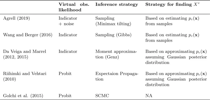
We give a brief overview of some alternative and related approaches to constrained GPs. For the approaches that rely on imposing constraints at a finite set of virtual observation locations, we recall that the constraint probability can be used in the search for a suitable set of virtual observation locations. The constraint probability is the probability that the constraint holds at an arbitrary input x, pc(x) given in (11). Some key characteristics of the approaches that make use of virtual observations are summarized in Table 1.
The related work most similar to the approach presented in this paper is that of Wang and Berger (2016) and Da Veiga and Marrel (2012, 2015). Wang and Berger (2016) make use of a similar sampling scheme for noiseless GP regression applied to computer code emulation. A Gibbs sampling procedure is used for inference and to estimate the constraint probability
pc(x) in the search for virtual observation locations. The approach of Da Veiga and Marrel (2012, 2015) is based on computation of the posterior mean and covariance of the constrained GP, using the equations that are also restated in this paper in Corollary 6. They make use of a Genz approximation for inference (Genz, 1992, 1997), and also introduce a crude but faster correlation-free approximation that can be used in the search for virtual observation locations. The approach of Da Veiga and Marrel (2012, 2015) is discussed further in the numerical experiments below, where we illustrate the idea in Example 1 and in Example 2 study an approximation of the posterior constrained GP using the constrained moments with a Gaussian distribution assumption. A major component in (Da Veiga and Marrel, 2012, 2015), (Wang and Berger, 2016) and this paper is thus computation involving the truncated multivariate Gaussian. Besides the choice of method for sampling from this distribution, the main difference with our approach is that we leverage Cholesky factorizations and noisy virtual observations for numerical stability.
Virtual obs. likelihood
Inference strategy Strategy for findingXv
Agrell (2019) Indicator Sampling Based on estimatingpc(x)
+ noise (Minimax tilting) from samples
Wang and Berger (2016) Indicator Sampling (Gibbs) Based on estimatingpc(x)
from samples
Da Veiga and Marrel Indicator Moment approxima- Based on approximatingpc(x)
(2012, 2015) tion (Genz) assuming Gaussian posterior distribution
Riihimki and Vehtari Probit Expectaion Propaga- Based on approximatingpc(x)
(2010) tion assuming Gaussian posterior distribution
Golchi et al. (2015) Probit SCMC NA
Table 1: Summary of alternative approaches that make use of virtual observations. The table compares the likelihood used for virtual observations, the method used for inference and to determine the set of virtual observation locationsXv.
2015; Riihimki and Vehtari, 2010), is that for practical applications in more than a few dimensions, such a strategy is essential to avoid numerical issues related to high serial correlation, and also to reduce the number of virtual observation locations needed. It is also worth noting that a strategy that decouples computation involving training data and virtual observation locations from inference at new locations is beneficial. For the approaches discussed herein that rely on sampling/approximation related to the truncated multivariate Gaussian, the samples/approximations can be stored and reused as discussed in Section 3.8.
There are also some approaches to constrained GPs that are not based on the idea of using virtual observations. An interesting approach by Maatouk and Bay (2017), that is also followed up by L´opez-Lopera et al. (2018), is based on modelling a conditional process where the constraints hold in the entire domain. They achieve this through finite-dimensional approximations of the GP that converge uniformly pathwise. With this approach, sampling from a truncated multivariate Gaussian is also needed for inference, in order to estimate the coefficients of the finite-dimensional approximation that arise from discretization of the input space. The authors give examples in 1D and 2D, but note that due to the structure of the approximation, the approach will be time consuming for practical applications in higher dimensions. There are also other approaches that consider special types of shape constraints, but where generalization seems difficult. See for instance (Abrahamsen and Benth, 2001; Yoo and Kyriakidis, 2006; Michalak, 2008; Kleijnen and Beers, 2013; Lin and Dunson, 2014; Lenk and Choi, 2017).
4.2. Numerical Experiments
• a0(x)≤f(x)≤b0(x)
• ai(x)≤∂f /∂xi(x)≤bi(x)
for all x in some bounded subset of Rnx, and i ∈ I ⊂ {1, . . . , nx}. Without loss of gen-erality we assume that the constrains on partial derivatives are with respect to the first k
components of x, i.e. I ={1, . . . , k}for somek≤nx.
As the prior GP we will assume a constant meanµ= 0 and make use of either the RBF or Mat´ern 5/2 covariance function. These are stationary kernels of the form
K(x,x0) =σK2k(r), r=
v u u t nx X i=1
xi−x0i
li
2
, (16)
with variance parameter σK2 and length scale parameters li for i = 1, . . . , nx. The radial basis function (RBF), also called squared exponential kernel, and the Mat´ern 5/2 kernel are defined through the function k(r) as
kRBF(r) =e−
1 2r
2
and kMat´ern 5/2(r) = (1 + √
5r+5 3r
2)e−√5r.
In general, the kernel hyperparameters σK2 and li are optimized together with the noise variance σ through MLE. In the examples that consider noiseless observations, the noise variance is not estimated, but set to a small fixed value as discussed in Section 3.8. With the above choice of covariance function, existence of the transformed GP is ensured. In fact, the resulting process is infinitely differentiable using the RBF kernel (see Adler, 1981, Theorem 2.2.2) and twice differentiable with the Mat´ern 5/2. These prior GP alternatives were chosen as they are the most commonly used in the literature, and thus a good starting point for illustrating the effect of including linear constraints. We note that although it is not in general possible to design mean and covariance functions that produce GPs that satisfy the constraints considered in this paper, one could certainly ease numerical computations by selecting a GP prior based on the constraint probability p(C|Y, θ) in (7), and for instance make us of a mean function that is known to satisfy the constraint.
If we let F0f = f, Fif = ∂f /∂x
i, and Xv,i be the set of Si virtual observations corresponding to thei-th operatorFi, then we can make use of the formulation in Section 3.5 and equations from Appendix C to obtain
Lµv = [µ1S0,0S[1,k]] T,
where1S1 is the vector [1, . . . ,1]T of lengthS1 and0S[1,k] is the vector [0, . . . ,0]
T of length
S[1,k]=−S0+PSi. Furthermore,
KX,XvLT =
h
KX,Xv,0,(K
1,0
Xv,1,X)
T, . . . ,(Kk,0
Xv,k,X)
Ti,
KX∗,XvLT =
h
KX∗,Xv,0,(K
1,0
Xv,1,X∗)T, . . . ,(K
k,0
Xv,k,X∗)T
i ,
LKXv,XvLT =
KXv,0,Xv,0 (K1,0
Xv,1,Xv,0)T . . . (K
k,0
Xv,k,Xv,0)T
KX1,0v,1,Xv,0 K
1,1
Xv,1,Xv,1 . . . K
1,k Xv,1,Xv,k
..
. ... . .. ...
KXk,0v,k,Xv,0 K
k,1
Xv,k,Xv,1 . . . K
k,k Xv,k,Xv,k
where we have used the notation
Ki,0(x,x0) = ∂
∂xi
K(x,x0) and Ki,j(x,x0) = ∂
2
∂xi∂x0i
K(x,x0).
The use of constraints related to boundedness and monotonicity is illustrated using three examples of GP regression. Example 1 considers a function f :R→Rsubjected to bound-edness and monotonicity constraints. In Example 2 a function f : R4 → R is estimated under the assumption that information on whether the function is monotone increasing or decreasing as a function of the first two inputs is known, i.e. sgn(∂f/∂x1) and sgn(∂f/∂x2)
are known. In Example 3 we illustrate how monotonicity constraints in multiple dimensions can be used in prediction of pressure capacity of pipelines.
4.2.1. Example 1: Illustration of Boundedness and Monotonicity in 1D
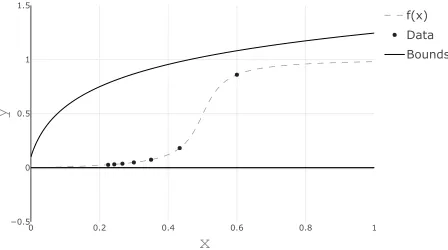
As a simple illustration of imposing constraints in GP regression, we first consider the function f :R→ Rgiven by f(x) = 13[tan−1(20x−10)−tan−1(−10)]. We assume that the function value is known at 7 input locations given by xi = 0.1 + 1/(i+ 1) for i= 1, . . . ,7. First, we assume that the observations are noiseless, i.e. f(xi) is observed for each xi. Estimating the function that interpolates at these observations is commonly referred to as emulation, which is relevant when dealing with data from computer experiments. Our function f(x) is both bounded and increasing on all ofR. In this example we will constrain the GP to satisfy the conditions that for x ∈ [0,1], we have that df/dx ≥ 0 and a(x) ≤
f(x)≤b(x) for a(x) = 0 and b(x) = 13ln(30x+ 1) + 0.1. The function is shown in Figure 1 together with the bounds and the 7 observations.
0 0.2 0.4 0.6 0.8 1
−0.5 0 0.5 1 1.5
f(x) Data Bounds
x
y
Figure 1: Function to emulate in Example 1
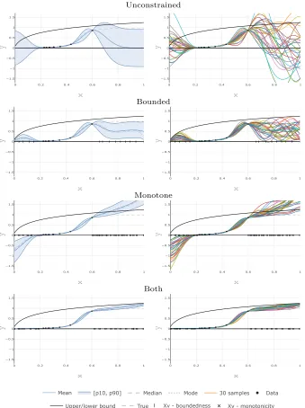
kernel density estimator over the samples generated in Algorithm 3. For both constraints, 17 locations was needed for monotonicity and only 3 locations was needed to impose bound-edness when the virtual locations for both constraints where optimized simultaneously. This is reasonable, as requiring f(0) > 0 is sufficient to ensure f(x) > 0 for x ≥ 0 when f is increasing, and similarly requiring f(xv) < b(xv) for some few points xv ∈ [0.6,1] should suffice. But note that Algorithm 7 finds the virtual observation locations for both con-straints simultaneously. Herexv = 0 for boundedness was first identified, followed by some few points for monotonicity, followed by a new pointxv for boundedness etcetera.
For illustration purposes none of the hyperparameters of the GP were optimized. More-over, for data sets such as the one in this example using plug-in estimates obtained from MLE generally not appropriate due to overfitting. Maximizing the marginal likelihood for the unconstrained GP gives a very poor model upon visual inspection (σK = 0.86, l= 0.26). However, it was observed that the estimated parameters for the constrained model (us-ing Eq. (8)) gives estimates closer to the selected prior which seems more reasonable (σK = 0.42, l = 0.17), and hence the inclusion of the constraint probability, p(C|Y, θ), in the likelihood seems to improve the estimates also for the unconstrained GP.
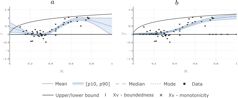
We may also assume that the observations come with Gaussian white noise, which in terms of numerical stability is much less challenging than interpolation. Figure 3 shows the resulting GPs fitted to 50 observations. The observations were generated by samplingxi ∈ [0.1,0.8] uniformly, andyifrom f(xi)+εiwhereεiare i.i.d. zero mean Gaussian with variance
0 0.2 0.4 0.6 0.8 1 −1.5 −1 −0.5 0 0.5 1 1.5 x y
0 0.2 0.4 0.6 0.8 1 −1.5 −1 −0.5 0 0.5 1 1.5 x y Unconstrained
0 0.2 0.4 0.6 0.8 1 −1.5 −1 −0.5 0 0.5 1 1.5 x y
0 0.2 0.4 0.6 0.8 1 −1.5 −1 −0.5 0 0.5 1 1.5 ss x y Bounded
0 0.2 0.4 0.6 0.8 1 −1.5 −1 −0.5 0 0.5 1 1.5 x y
0 0.2 0.4 0.6 0.8 1 −1.5 −1 −0.5 0 0.5 1 1.5 ty x y Monotone
0 0.2 0.4 0.6 0.8 1 −1.5 −1 −0.5 0 0.5 1 1.5 x y
0 0.2 0.4 0.6 0.8 1 −1.5 −1 −0.5 0 0.5 1 1.5 ss ty x y Both [p10, p90] Mean True Data
Xv - boundedness Xv - monotonicity Mode
Median 30 samples
Upper/lower bound
Figure 2: The GP with parameters σK = 0.5 (variance) andl = 0.1 (length scale) used in Example 1. The virtual observation locations are indicated by markers on the
0 0.2 0.4 0.6 0.8 1 −1.5
−1 −0.5 0 0.5 1 1.5
x
y
0 0.2 0.4 0.6 0.8 1
−1.5 −1 −0.5 0 0.5 1 1.5
ss ty
x
y
a b
[p10, p90]
Mean Data
Xv - boundedness Xv - monotonicity Mode
Median
Upper/lower bound
Figure 3: Unconstrained (a) and constrained (b) GPs fitted to 50 observations with Gaus-sian noise. The predictive distributions are shown, i.e. the distribution of f(x) wherey=f(x) +ε.
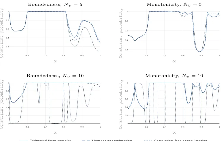
Da Veiga and Marrel (2015) propose to use estimates of the posterior mean and variance ofLf(x)|Y, C to estimate the constraint probabilitypc(x) assuming a Gaussian distribution. They also introduce the faster correlation-free approximation, where the parameters are estimated under the assumption that observations of Lf(x)|Y at different input locations
0.2 0.4 0.6 0.8 1 0.2 0.4 0.6 0.8 1 x Constraint probability
0.2 0.4 0.6 0.8 1 0.2 0.4 0.6 0.8 1 x Constraint probability
Boundedness,Nv = 5 Monotonicity,Nv= 5
0.2 0.4 0.6 0.8 1 0 0.2 0.4 0.6 0.8 1 x Constraint probability
0.2 0.4 0.6 0.8 1 0 0.2 0.4 0.6 0.8 1 x Constraint probability
Boundedness, Nv = 10 Monotonicity,Nv = 10
Figure 4: Constraint probabilitypc(x) computed using the estimate (13) together with the moment based approximations from Da Veiga and Marrel (2015). The constraint probability is shown for monotonicity and boundedness, where Nv is the total number of virtual observation locations used in the model.
4.2.2. Example 2: 4D Robot Arm Function
In this example we consider emulation of a function f : R4 → R, where we assume that the sign of the first two partial derivatives, sgn(∂f/∂x1) and sgn(∂f/∂x2), are known. The
function to emulate is
f(x) = m X
i=1
Li cos
i X j=1 τj ,
form= 2, andx= [L1, L2, τ1, τ2]. The function is inspired by the robot arm function often
used to test function estimation (An and Owen, 2001). Here f(x) is the y-coordinate of a two dimensional robot arm withm line segments of length Li ∈ [0,1], positioned at angle
τi ∈ [0,2π] with respect to the horizontal axis. The constraints on the first two partial derivatives thus implies that it is known whether or not the arm will move further away from the x-axis, as a function of the arm lengths,L1 andL2, for any combination ofτ1 and
τ2.
candi-date set of 1000 locations in the minimization of the constraint probability. We repeat this procedure 100 times and report performance using the predictivity coefficientQ2, predictive variance adequation (PVA) and the average width of 95% confidence intervals (AWoCI).
Given a set of tests y1, . . . , yntest and predictions ˆy1, . . . ,yˆntest,Q
2 is defined as
Q2 = 1−
ntest X
i=1
(ˆyi−yi)2/ ntest
X
i=1
(¯y−yi)2,
where ¯yis the mean of y1, . . . , yntest. In our experiments the predictions ˆyi are given by the
posterior mean of the GP. The PVA criterion is defined as
PVA =
log 1
ntest
ntest X
i=1
(ˆyi−yi)2 ˆ
σ2
i !
,
where ˆσ2i is the predictive variance. This criterion evaluates the quality of the predictive variances and to what extent confidence intervals are reliable. The smaller the PVA is, the better (Bachoc, 2013). In addition to this criterion, it is also useful to evaluate the size of confidence intervals. For this we compute the average width of 95% confidence intervals
AWoCI = 1
ntest
ntest X
i=1
(p(0i.)975−p(0i.)025),
wherep(0i.)975 and p0(i.)025 are the predicted 97.5% and 2.5% percentiles.
The result of 100 predictions for one single experiment is shown in Figure 5. As ex-pected, the estimated prediction uncertainty is reduced significantly using the constrained model, and single predictions given by the posterior mean are also improved. In Table 2 we summarize the results from running 100 of these experiments. In each experiment,Q2, PVA and AWoCI was computed from prediction at 1000 locations sampled uniformly in the domain. We also report the probability that the constraint holds in the unconstrained GP, p(C|Y) given in (7), and the CPU time in seconds used to generate 104 samples from the posterior on an IntelR CoreTMi5-7300U 2.6GHz CPU. For comparison, we also include
predictions from moment-based approximations using the approach of Da Veiga and Marrel (2012, 2015). We study in particular their approach for finding the set of virtual observation locations, as discussed in Section 3.7 and illustrated in the previous example. In total, the following alternatives are considered:
1. Unconstrained: The initial GP without constraints.
2. Constrained: The constrained GP using the approach presented in this paper. 3. Moment approx. 1: Using the sampling scheme of this paper for inference, but
where the moment based approximation is used in the search for virtual observation locations.
5. Correlation-free approx.: Same asMoment approx. 1but where the correlation-free approximation is used in the search for virtual observation locations.
−2 −1 0 1 2 −2
−1 0 1 2
Standard normal quantiles
Sample quantiles
−1 −0.5 0 0.5 1 −1.5
−1 −0.5 0 0.5 1 1.5
True value
Predicted
value
−1 −0.5 0 0.5 1 −1.5
−1 −0.5 0 0.5 1 1.5
True value
Predicted
value
a
b
c
Figure 5: Figure ashows a qq-plot with 95% confidence band of 100 normalized residuals (yi −µi)/(σi), where µi and σi2 are the mean and variance of the predictive distribution of the unconstrained GP. In Figureb, predictions vs the true function value is shown together with a [0.025,0.975] (95%) percentile interval for the unconstrained GP. The same type of figure is shown incfor the constrained GP.
In Table 2 we see that the use of constraints is beneficial in terms of both a higher Q2
p(C|Y) Ts PVA Q2 AWoCI
Unconstrained 3.03 0.7558 0.99
Constrained 4.1E-34 24.8 2.85 0.8842 0.54
Moment approx. 1 2.4E-36 25.2 2.84 0.8844 0.54
Moment approx. 2 2.4E-36 25.2 2.84 0.8844 0.83
correlation-free approx. 8.6E-37 21.1 2.91 0.8775 0.55
Table 2: Average values from 100 experiments of the robot arm function. Ts is the CPU time in seconds used to generate 104 samples.
Unconstrained Constrained Correlation free approx. Moment approx. 1 Moment approx. 2
0.4 0.5 0.6 0.7 0.8 0.9 1 1.1 1.2
AWoCI
Figure 6: Average width of confidence intervals (AWoCI) from 100 experiments of the robot arm function.
4.2.3. Example 3: Pipeline Pressure Capacity
In this example we consider a model for predicting the pressure capacity of a steel pipeline with defects due to corrosion. As corrosion is one of the major threats to the integrity of offshore pipelines, experiments are carried out to understand how metal loss due to corrosion affects a pipeline’s capacity with respect to internal pressure (Sigurdsson et al., 1999; Amaya et al., 2019). These include full scale burst tests and numerical simulation through Finite Element Analysis (FEA). Results from this type of experiments serve as the basis for current methodologies used in the industry for practical assessment of failure probabilities related to pipeline corrosion, such as ASME B31G or DNVGL-RP-F101. We consider experiments related to a single rectangular shaped defect, which is essential to these methodologies.
bursting is in the simplified equation given as
Pcap(σu, D, t, d, l) = 1.05
2tσu
D−t
1−d/t
1−d/tQ , Q=
r
1 + 0.31 l
2
Dt,
where σu ∈[450,550] (MPa) is the ultimate tensile strength of the material,D∈[10t,50t] (mm) and t∈ [5,30] (mm) are the outer diameter and wall thickness of the pipeline, and
d∈[0, t] (mm) and l∈[0,1000] (mm) are the depth and length of the rectangular defect. From the physical phenomenon under consideration, we know that the capacity of the pipeline will decrease if the size of the defect were to increase. Similarly, we know that the pipeline capacity increases with a higher material strength or wall thickness, and decreases as a function of the diameter, all else kept equal. In the form of partial derivatives we can express this information as: ∂Pcap
∂d <0, ∂Pcap
∂l <0, ∂Pcap
∂σu >0,
∂Pcap
∂t >0 and ∂Pcap
∂D <0. For convenience we will transform the input variables to the unit hypercube. Let x
denote the transformed input vector x= [x1, . . . , x5], where x1 = (σu−450)/(550−450),
x2 = (D/t−10)/(50−10),x3= (t−5)/(30−5), x4 =d/tand x5 =l/1000. We will make
use of the function
f(x) =Pcap(x) for x∈[0,1]5,
and assume that the burst capacity observed in an experiment is f(x) +ε, where ε is a zero mean Normal random variable with variance σ2 = 4. The constraints on the partial derivatives after the transformation becomes: ∂x1∂f > 0, ∂x2∂f < 0, ∂x3∂f > 0, ∂x4∂f < 0 and
∂f
∂x5 <0 for x∈[0,1]5.
In this example we thus have five constraints available, represented by bounds on the partial derivative of f(x) w.r.t. xi fori= 1, . . . ,5. Besides studying the effect of including all five constraints, we will test some different alternatives using a smaller number of con-straints, and also lower input dimensions. To simulate a lower dimensional version of the capacity equation, we can consider only the fistnx input variables and keep the remaining variables fixed. We consider nx= 3,4 and 5 where we fix xi = 0.5 for all i > nx. For each of these scenarios we will consider nx and nx−1 number of constraints. We letnc denote the number of constraints, where using nc constraints means that the bound on ∂f /∂xi is included fori= 1, . . . , nc.
In each experiment we start by generating a training set of N = 5nx or N = 10nx LHS samples from [0,1]nx. As in the previous example in Section 4.2.2, we fit a zero
mean GP using a Mat´ern 5/2 covariance function and plug-in hyperparameters by MLE. We search over a candidate set consisting of 2500 uniform samples from [0,1]nx iteratively
to update the set of virtual observation locations, until the constraint probability at all locations in the candidate set, and for each constraint, is at least 0.7. To check whether this is a reasonable stopping criterion we finish by minimizing the constraint probability for each constraint, using the differential evolution (Storn and Price, 1997) global optimization algorithm available in (SciPy Jones et al., 2001–).
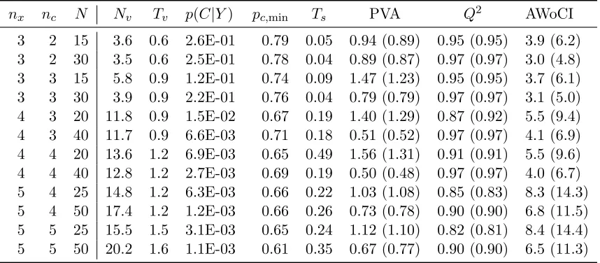
Table 3 shows the results for different combinations of input dimensionality nx, number of constraints nc and number of training samples N, where the results in each row is computed from 100 experiments. As in the previous example we report p(C|Y), PVA, Q2
nx nc N Nv Tv p(C|Y) pc,min Ts PVA Q2 AWoCI
3 2 15 3.6 0.6 2.6E-01 0.79 0.05 0.94 (0.89) 0.95 (0.95) 3.9 (6.2)
3 2 30 3.5 0.6 2.5E-01 0.78 0.04 0.89 (0.87) 0.97 (0.97) 3.0 (4.8)
3 3 15 5.8 0.9 1.2E-01 0.74 0.09 1.47 (1.23) 0.95 (0.95) 3.7 (6.1)
3 3 30 3.9 0.9 2.2E-01 0.76 0.04 0.79 (0.79) 0.97 (0.97) 3.1 (5.0)
4 3 20 11.8 0.9 1.5E-02 0.67 0.19 1.40 (1.29) 0.87 (0.92) 5.5 (9.4)
4 3 40 11.7 0.9 6.6E-03 0.71 0.18 0.51 (0.52) 0.97 (0.97) 4.1 (6.9)
4 4 20 13.6 1.2 6.9E-03 0.65 0.49 1.56 (1.31) 0.91 (0.91) 5.5 (9.6)
4 4 40 12.8 1.2 2.7E-03 0.69 0.19 0.50 (0.48) 0.97 (0.97) 4.0 (6.7)
5 4 25 14.8 1.2 6.3E-03 0.66 0.22 1.03 (1.08) 0.85 (0.83) 8.3 (14.3)
5 4 50 17.4 1.2 1.2E-03 0.66 0.26 0.73 (0.78) 0.90 (0.90) 6.8 (11.5)
5 5 25 15.5 1.5 3.1E-03 0.65 0.24 1.12 (1.10) 0.82 (0.81) 8.4 (14.4)
5 5 50 20.2 1.6 1.1E-03 0.61 0.35 0.67 (0.77) 0.90 (0.90) 6.5 (11.3)
Table 3: Average values from 100 experiments with input dimensionality nx, number of constraints nc and number of training samples N. Values in parenthesis corre-spond to the unconstrained model. Here pc,min is the minimum of the constraint
probability for any constraint over the entire domain after a total of Nv virtual observation locations have been included. Tv is the average CPU time in seconds used to find each of the Nv points using 103 samples, and Ts is the CPU time in seconds used to generate 104 samples of the final model for prediction.
the minimum constraint probability,pc,min = mini=1,...ncminx∈[0,1]nxpˆc,i(x) (13), computed
with differential evolution. Here we make use of 103samples to compute the estimate ˆpc,i(x), whereas 104 samples are used for the final prediction.
From Table 3 we first notice that the number of virtual observation locations (Nv) de-termined by the searching algorithm is fairly low. One might interpret this as an indication that the unconstrained GP produces samples that are likely to agree with the monotonicity constraints, except for at a few locations. As a result, computation that involve sampling from the truncated multivariate Gaussian is efficient. Still, we see that inclusion of the con-straints has an effect on uncertainty estimates as the AWoCI is reduced by a factor of around 1.6 in each experiment, whereas PVA andQ2 are fairly similar for the unconstrained and
constrained model overall. We also notice that the smallest constraint probability found in the domain using a global optimization technique is reduced when the number of constraints or dimensionality is increased. This is expected, as we only considered a finite candidate set and not the entire domain when searching for the location minimizing the constraint probability. Hence, if we really want to achieve a minimal constraint probability larger than 0.7 in 5 dimensions, more than 2500 samples in the candidate set would be needed with this strategy, or a global optimizer could be used to identify the remaining virtual observation locations needed.
make use of capacity predictions as the one illustrated in this example are usually derived in the context of Structural Reliability Analysis (SRA), where the capacity is combined with a probabilistic representation of load (in this case differential pressure) to estimate the probability of failure (Madsen et al., 2006).
Alternative methods based on conservative estimates to ensure sufficient safety margin between load and capacity are also common. For the application considered herein, this would typically mean using a lower percentile instead of the posterior mean in order to represent a conservative capacity. The inclusion of constraints can therefore help to avoid unnecessary conservatism due to unphysical scenarios, that are not realistic but have positive probability in the unconstrained model.
Finally, we note that the constraints used in this example are not from differentiating the equation used as stand-in for experiments, but from knowledge related to the underlying physical phenomenon. The constraints therefore remain applicable, were the experiments to come from physical full-scale tests. This naturally also holds in applications to computer code emulation, where we would set the noise term ε to zero in this example if we were to assume that the capacity experiments came from a numerical (FEA) simulation. With results from this type of numerical simulation, a noise parameter is usually added to the simulation output as well, to represent model uncertainty as the numerical simulation is not a perfect representation of the real physical phenomenon. Very often the model uncertainty is represented by a univariate Gaussian. An interesting alternative here is to instead account for the model uncertainty as observational noise in the GP, where the use of constraints may help to obtain a more realistic model uncertainty as well.
5. Discussion
suitable approximation-based algorithms. As for the simulation scheme in this paper, the only computational burden lies in sampling from a truncated multivariate Gaussian. As this is a fairly general problem, multiple good samplers exist for this purpose. We found the method of Botev (2017) to work particularly well for our applications, as it provides exact sampling in a relevant range of dimensions where many alternative sampling schemes fail. Based on a comparison made by L´opez-Lopera et al. (2018), we see that the method based on Hamiltonian Monte Carlo by Pakman and Paninski (2012) may also be appropriate.
As we discuss briefly in Section 3.3, estimation of hyperparameters becomes challenging when the termp(C|Y, θ) enters the likelihood. Moreover, as our approach is based on the use of virtual observation locations, we are aware that the task of estimating or optimiz-ing model hyperparameters in general is not well defined. This is because the likelihood depends both on the hyperparameters and the set of virtual observation locations (Eq. 8). This problem is neglected in the literature on shape-constrained GPs, where it is either assumed that the virtual observation locations are known a priori (for low input dimension selecting a space filling sufficiently dense design is unproblematic), or the hyperparameters are addressed independently of these. To our knowledge the problem of simultaneously estimating hyperparameters and virtual observation locations has not yet been addressed. A rather simplistic approach is to iterate between estimating hyperparameter and the set of virtual observation locations. However, for higher input dimensions this might be prob-lematic altogether, in which case sparse approximations may be needed to deal with a large set of virtual observation locations. In this setting, it might be more fruitful to view the virtual observation locations as additional hyperparameters, in a model approximating the posterior corresponding to an sufficiently dense set of virtual observation locations, e.g. as in the inducing points framework for scaling GPs to large data sets (de G. Matthews et al., 2016). This is a topic of further research.
With the approach in this paper, we make use of the probability p(C|Y), which is interesting in its own for investigating whether constraints such as e.g. monotonicity are likely to hold given a set of observations. Alternatively, inference on the constraint noise parameterσv can provide similar type of information. Ideally, we choose a small fixed value forσv to avoid numerical instability, as discussed in Section 3.8. But in extreme cases, with conflicting constraints or observations that contradict constraints with high probability, the model may still experience numerical issues. We argue that models that ’break’ under these circumstances are preferred as it reveals that either 1) there is something wrong with the observations, or 2) there is something wrong with the constraints and hence our knowledge of the underlying phenomenon (Agrell et al., 2018). It would nevertheless be better if more principled ways of investigating such issues were available. In our experiments we observed that the conditional likelihood, p(Y|C), in general is decreasing as a function of
σv, whereas this was not the case for an invalid constraint assuming a monotonicdecreasing function in Example 1. Hence, σv might provide useful information in this manner. The estimated partial constraint probabilities ˆpc,i(x) can also be useful for revealing such issues, for instance by monitoring the intermediate minimum values p∗i computed in Algorithm 7 as new virtual observation locations are added.
f :Rnx →Rny in a natural way. But for non-Gaussian likelihoods, or applications with large or high-dimensional data, other approximation based alternatives are needed.
Acknowledgments
This work has been supported by grant 276282 from the Norwegian Research Council and DNV GL Group Technology and Research. The research is part of an initiative on apply-ing constraints based on phenomenological knowledge in probabilistic machine learnapply-ing for high-risk applications, and the author would like to thank colleagues at DNV GL and the University of Oslo for fruitful discussions on the topic. A special thanks to Arne B. Huseby, Simen Eldevik, Andreas Hafver, and the editor and reviewers of JMLR for insightfull com-ments that have greatly improved the paper.
Appendix A. Proof of Lemma 1
Proof. We start by observing that (f∗,C, Ye ) is jointly Gaussian with mean and covariance
E([f∗,C, Ye ]T) = [µ∗,Lµv, µ]T, (17)
cov([f∗,C, Ye ]T) =
KX∗,X∗ KX∗,XvLT KX∗,X
LKXv,X∗ LKXv,XvLT +σ2
vINv LKXv,X
KX,X∗ KX,XvLT KX,X+σ2IN
. (18)
By first conditioning on Y we obtain
f∗
e C
Y ∼ N
µ∗+A2(Y −µ)
Lµv+A1(Y −µ)
,
B2 B3
B3T B1
, (19)
forA1= (LKXv,X)(KX,X+σ2IN)−1,A2 =KX∗,X(KX,X+σ2IN)−1,B1 =LKXv,XvLT + σv2INv−A1KX,XvLT,B2=KX∗,X∗−A2KX,X∗, and B3=KX∗,XvLT −A2KX,XvLT.
Conditioning on Ce then gives
f∗|Y,Ce∼ N
µ∗+A(Ce− Lµv) +B(Y −µ),Σ
, (20)
forA=B3B1−1,B =A2−AA1 and Σ =B2−AB3T.
Similarly, we may derive Ce|Y by observing that the joint distribution ofC, Ye is given by removing the first row in (17) and the first row and column in (18). Hence,
e
C|Y ∼ N(Lµv+A1(Y −µ), B1). (21)