Patchwork Kriging for Large-scale Gaussian Process Regression

Patchwork Kriging for Large-scale Gaussian Process

Regression

Chiwoo Park [email protected]

Department of Industrial and Manufacturing Engineering Florida State University

2525 Pottsdamer St., Tallahassee, FL 32310-6046, USA.

Daniel Apley [email protected]

Dept. of Industrial Engineering and Management Sciences Northwestern University

2145 Sheridan Rd., Evanston, IL 60208-3119, USA.

Editor:Neil Lawrence

Abstract

This paper presents a new approach for Gaussian process (GP) regression for large datasets. The approach involves partitioning the regression input domain into multiple local regions with a different local GP model fitted in each region. Unlike existing local partitioned GP approaches, we introduce a technique for patching together the local GP models nearly seamlessly to ensure that the local GP models for two neighboring regions produce nearly the same response prediction and prediction error variance on the boundary between the two regions. This largely mitigates the well-known discontinuity problem that degrades the prediction accuracy of existing local partitioned GP methods over regional boundaries. Our main innovation is to represent the continuity conditions as additional pseudo-observations that the differences between neighboring GP responses are identically zero at an appropri-ately chosen set of boundary input locations. To predict the response at any input location, we simply augment the actual response observations with the pseudo-observations and ap-ply standard GP prediction methods to the augmented data. In contrast to heuristic continuity adjustments, this has an advantage of working within a formal GP framework, so that the GP-based predictive uncertainty quantification remains valid. Our approach also inherits a sparse block-like structure for the sample covariance matrix, which results in computationally efficient closed-form expressions for the predictive mean and variance. In addition, we provide a new spatial partitioning scheme based on a recursive space par-titioning along local principal component directions, which makes the proposed approach applicable for regression domains having more than two dimensions. Using three spatial datasets and three higher dimensional datasets, we investigate the numerical performance of the approach and compare it to several state-of-the-art approaches.

Keywords: Local Kriging, Model Split and Merge, Pseudo Observations, Spatial Parti-tion

1. Introduction

Gaussian process (GP) regression is a popular Bayesian nonparametric approach for non-linear regression (Rasmussen and Williams, 2006). A GP prior is assumed for the unknown regression function, and the posterior estimate of the function is from this prior, combined

c

with noisy (or noiseless, for deterministic simulation response surfaces) response obser-vations. The posterior estimate can be easily derived in a simple closed form using the properties induced by the GP prior, and the estimator has several desirable properties, e.g., it is the best linear unbiased estimator under the assumed model and offers convenient quantification of the prediction error uncertainty. Its conceptual simplicity and attractive properties are major reasons for its popularity. On the other hand, the computational

expense for evaluating the closed form solution is proportional to N3, where N denotes

the number of observations, which can be prohibitively expensive for large N. Broadly

speaking, this paper concerns fast computation of the GP regression estimate for large N.

The major computational bottleneck for GP regression is the inversion of a N ×N

sample covariance matrix, which is also often poorly numerically conditioned. Different approaches for representing or approximating the sample covariance matrix with a more efficiently invertible form have been proposed. The approaches can be roughly categorized as sparse approximations, low-rank approximations, or local approximations. Sparse meth-ods represent the sample covariance with a sparse version, e.g. by applying a covariance tapering technique (Furrer et al., 2006; Kaufman et al., 2008), using a compactly supported covariance function (Gneiting, 2002), or using a Gaussian Markov approximation of a GP (Lindgren et al., 2011). The inversion of a sparse positive definite matrix is less computa-tionally expensive than the inversion of a non-sparse matrix of the same size, because its Cholesky decomposition is sparse and can be achieved more quickly.

Low-rank approximations of the sample covariance matrix can be performed in multiple ways. The most popular approach for the low-rank approximation introduces latent vari-ables and assume a certain independence conditioned on the latent varivari-ables (Seeger et al., 2003; Snelson and Ghahramani, 2006), so that the resulting sample covariance matrix has

reduced rank. The (pseudo)inversion of aN ×N matrix of rank M can be computed with

reducedO(N M2) expense. Titsias (2009) introduced a variational formulation to infer the

latent variables along with covariance parameters, and a variant of the idea was proposed using the stochastic variational inference technique (Hensman et al., 2013). The latent variable model approaches are exploited to develop parallel computing algorithms for GP regression (Chen et al., 2013). Another way for low rank approximation is to approxi-mate the sample covariance matrix with a product of a block diagonal matrix and multiple blocked low-rank matrices (Ambikasaran et al., 2016).

approach is to smooth out some of the discontinuity by using some weighted average across the local models or across multiple sets of local models via a Dirichlet mixture (Rasmussen and Ghahramani, 2002), a treed mixture (Gramacy and Lee, 2008), Bayesian model av-eraging (Tresp, 2000; Chen and Ren, 2009; Deisenroth and Ng, 2015), or locally weighted projections (Nguyen-Tuong et al., 2009). Other, related approaches use additive covariance functions consisting of a global covariance and a local covariance (Snelson and Ghahramani, 2007; Vanhatalo and Vehtari, 2008), construct a local model for each testing point (Gra-macy and Apley, 2015), or use a local partition but constrain the local models for continuity (Park et al., 2011; Park and Huang, 2016).

In this work we use a partitioned input domain like Park et al. (2011) and Park and Huang (2016), but we introduce a different form of continuity constraints that are more easily and more naturally integrated into the GP modeling framework. Both Park et al. (2011) and Park and Huang (2016) basically reformulated local GP regression as an op-timization problem, and the local GP models for neighboring regions were constrained to have the same predictive means on the boundaries of the local regions by adding some linear constraints to the optimization problems that infer the local GP models. Park et al. (2011) used a constrained quadratic optimization that constrains the predictive means for a finite number of boundary locations, and Park and Huang (2016) introduced a functional optimization formulation to enforce the same constraints for all boundary locations. The optimization-based formulations make it infeasible to derive the marginal likelihood and the predictive variances in closed forms, which were roughly approximated. In contrast, this paper presents a simple and natural way to enforce continuity. We consider a set of GPs that are defined as the differences between the responses for the local GPs in neighboring regions. Continuity implies that these differenced GPs are identically zero along the bound-ary between neighboring regions. Hence, we impose continuity constraints by treating the values of the differenced GPs at a specified set of boundary points as all having been “ob-served to be zero”, and we refer to these zero-valued differences as pseudo-observations. We can then conveniently incorporate continuity constraints by simply augmenting the actual set of response observations with the set of pseudo-observations, and then using standard GP modeling to calculate the posterior predictive distribution given the augmented set of

observations. We note that observing the differenced GPs to be zero at a set of boundary

points is essentially equivalent toassuming continuity at these points without imposing any

further assumptions on the nature of the GPs.

only applicable for one- or two-dimensional problems, while our new approach is applicable for higher dimensional regression problems. We view our approach as “patching” together a collection of local GP regression models using the boundary points as “stitches”, and,

hence, we refer to it aspatchwork kriging.

The remainder of the paper is organized as follows. Section 2 briefly reviews the general GP regression problem and notational convention. Section 3 presents the core methodology of the patchwork kriging approach, including the prior model assumptions, the pseudo-observation definition, the resulting posterior predictive mean and variance equations, and the detailed computation steps along with choice of tuning parameters. Section 4 shows how the patchwork kriging performs with a toy example for illustrative purpose. Section 5 investigates the numerical performance of the proposed method for different simulated cases and compares it with the exact GP regression (i.e., the GP regression without partitions, using the entire dataset to predict each point) and a global GP approximation method. Section 6 presents the numerical performance of the proposed approach for five real datasets and compares it with Park and Huang (2016) and other state-of-the-art methods. Finally, Section 7 concludes the paper with a discussion.

2. Gaussian Process Regression

Consider the general regression problem of estimating an unknown predictive function f

that relates addimensional predictorx∈Rd to a real responsey, using noisy observations

D={(xi, yi), i= 1, . . . , N},

yi =µ+f(xi) +i, i= 1, . . . , N,

wherei∼ N(0, σ2) is white noise, independent off(xi). We assume thatµ= 0. Otherwise,

one can normalizeyi by subtracting the sample mean of theyi’s fromyi. Notice that we do

not use bold font for the multivariate predictor xi and reserve bold font for the collection

of observed predictor locations,x= [x1, x2, . . . , xN]T.

In a GP regression for this problem, one assumes that f is a realization of a zero-mean

Gaussian process having covariance function c(·,·) and then uses the observations D to

obtain the posterior predictive distribution off at an arbitraryx∗, denoted byf∗=f(x∗).

Denotey= [y1, y2, . . . , yN]T. The joint distribution of (f∗,y) is

P(f∗,y) =N

0,

c∗∗ cTx∗

cx∗ σ2I +Cxx

,

where c∗∗=c(x∗, x∗), cx∗ = (c(x1, x∗), . . . , c(xN, x∗))T and Cxx is an N ×N matrix with

(i, j)thentryc(xi, xj). The subscripts onc∗∗,cx∗, andCxx indicate the two sets of locations

between which the covariance is computed, and we have abbreviated the subscript x∗ as∗.

Applying the Gaussian conditioning formula to the joint distribution gives the predictive

distribution of f∗ given y (Rasmussen and Williams, 2006),

P(f∗|y) =N(cx∗T (σ2I+Cxx)−1y, c∗∗−cTx∗(σ2I +Cxx)−1cx∗). (1)

The predictive mean cTx∗(σ2I +Cxx)−1y is taken to be the point prediction of f(x) at

location x∗, and its uncertainty is measured by the predictive variance c∗∗ −cTx∗(σ2I +

Cxx)−1cx∗. Efficient calculation of the predictive mean and variance for large datasets has

3. Patchwork Kriging

As mentioned in the introduction, for efficient computation we replace the GP regression by a set of local GP models on some partition of the input domain, in a manner that enforces a level of continuity in the local GP model responses over the boundaries separating their respective regions. Section 3.1 conveys the main idea of the proposed approach,

3.1 Inference with Boundary Continuity Constraints

To specify the idea more precisely, consider a spatial partition of the input domain off(x)

intoK local regions{Ωk:k= 1,2, ..., K}, and define fk(x) as the local GP approximation

of f(x) at x ∈ Ωk, where Ωk is the closure of Ωk. Temporarily ignoring the continuity

requirements, the local models are assumed to follow independent GP priors:

Assumption 1 Each fk(x) follows a GP prior distribution with zero mean and covariance

function ck(·,·), and the fk(x)’s are mutually independent a priori (prior to enforcing the

continuity conditions). The choice of the local covariance function(s) can differ depending on the specifics of the problem. If f(x) is expected to be a stationary process, then one could use the same ck(·,·) = c(·,·) for all k. In this case, the purpose of this local GP

approximation would be to approximatef(x)computationally efficiently. On the other hand, if one expects non-stationary behavior of the data, then different covariance functions should be used for each region.

It is important to note that the independence of the GPs in Assumption 1 is prior to enforcing the continuity conditions via the pseudo-observations, as described below. After

enforcing the continuity conditions, the GPs will no longer be independent a priori, since

the assumed continuity at the boundaries imposes a very strong prior dependence of the sur-faces. Since the pseudo-observations should also be viewed as additional prior information,

the independence condition in Assumption 1 might be more appropriately viewed as a

hy-perprior condition. In fact, we view the incorporation of the boundary pseudo-observations as an extremely tractable and straightforward way of imposing some reasonable form of

dependency of the fk(x) across regions (which is the ultimate goal), while still allowing

us to begin with an independent GP hyperprior (which results in the tractability of the

analyses).

Now partition the training set D into D_k = {(xi, yi) : xi ∈ Ωk} (k = 1,2, ..., K), and

denote xk = {xi : xi ∈ Ωk} and yk = {yi : xi ∈ Ωk}. By the independence part of

Assumption 1, the predictive distribution of fk(x) given D is equivalent to the predictive

distribution offk(x) givenDk, which gives the standard local GP solution with no continuity requirements. The primary problem with this formulation is that the predictive distributions of fk(x) and fl(x) are not equal on the boundary of their neighboring regions Ωk and Ωl.

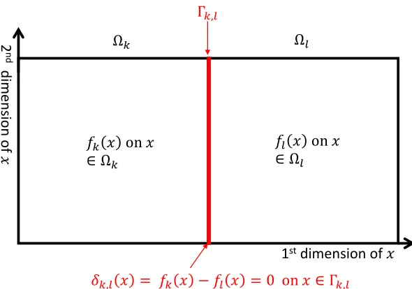
Our objective is to improve the local kriging prediction by enforcing fk(x) = fl(x) on their shared boundary. The key idea is illustrated in Figure 1 and described as follows. For

two neighboring regions Ωk and Ωl, let Γk,l = Ωk∩Ωl denote their shared boundary. For

each pair of neighboring regions Ωkand Ωl, we define the auxiliary processδk,l(x) to be the difference between the two local GP models,

Ω𝑘 Ω𝑙

𝑓𝑘 𝑥 on 𝑥

∈ Ω𝑘

Γ𝑘,𝑙

𝑓𝑙 𝑥 on 𝑥

∈ Ω𝑙

𝛿𝑘,𝑙 𝑥 = 𝑓𝑘 𝑥 − 𝑓𝑙 𝑥 = 0 on 𝑥 ∈ Γ𝑘,𝑙

1st_{dimension of 𝑥}

2

nd

d

ime

n

sion

of

𝑥

Figure 1: Illustration of the notation and concepts for defining the local models fk(x)

and fl(x). Ωk and Ωl represent two local regions resulting from some appropriate spatial

partition (discussed later) of the regression input domain. The (posterior distributions for the) GP functionsfk(x) and fl(x) represent the local approximations of the regression

function on Ωk and Ωl, respectively. The subset Γk,l represents the interfacial boundary

between the two regions Ωk and Ωl, and δk,l(x) is defined as the difference between fk(x) and fl(x), which is identically zero on Γk,l by the continuity assumption.

and it is only defined for k < l to avoid any duplicated definition of the auxiliary process.

By the definition and under Assumption 1, δk,l(x) is a Gaussian process with zero mean

and covariance functionck(·,·) +cl(·,·), and its covariance with fj(x) is

Cov(δk,l(x1), fj(x2)) =Cov(fk(x1)−fl(x1), fj(x2))

=Cov(fk(x1), fj(x2))−Cov(fl(x1), fj(x2)).

Since Cov(fk(x1), fl(x2)) =ck(x1, x2) for k=land zero otherwise under Assumption 1,

Cov(δk,l(x1), fj(x2)) =



 

 

ck(x1, x2) ifk=j −cl(x1, x2) ifl=j

0 otherwise.

(3)

Likewise,δk,l(x) and δu,v(x) are correlated with covariance

Cov(δk,l(x1), δu,v(x2)) =

          

         

ck(x1, x2) ifk=u, l6=v cl(x1, x2) ifl=v, k6=u

−ck(x1, x2) ifk=v, l6=u −cl(x1, x2) ifl=u, k6=v

ck(x1, x2) +cl(x1, x2) ifk=u, l=v

0 otherwise.

Boundary continuity betweenfk(x) andfl(x) can be achieved by enforcing the condition

δk,l(x) = 0 at Γj,k. We reiterate that fk(x) and fl(x) are no longer independent after conditioning on the additional informationδk,l(x) = 0. In fact, they are strongly dependent,

as they must be in order to achieve continuitya priori. Hence, the independence condition

in Assumption 1 is really ahyperprior independence.

Deriving the exact prior distribution of the surface conditioned onδk,l(x) = 0 everywhere on the boundaries appears to be computationally intractable, because there are uncountably

infinitely many x’s in Γj,k. Instead, we propose a much simpler continuity correction that

begins with the Assumption 1 prior (including the independencehyperprior) and augments

the observed data D with the pseudo observations δk,l(x) = 0 for a finite number of input

locations x ∈Γk,l. As the number of boundary pseudo-observations grows, we can better

approximate the theoretical ideal condition that δk,l(x) = 0 everywhere on the boundary.

The choice of the boundary input locations will be discussed later.

Notice that observing “δk,l(x) = 0” is equivalent to observing thatfk(x) =fl(x) without

observing the actual values of fk(x) and fl(x). Thus, if we augment D to include these

pseudo observations when calculating the posterior predictive distributions of fk(x) and

fl(x), it will force the posterior distributions of fk(x) and fl(x) to be the same at each

boundary input location x, because observing δk,l(x) = 0 means that we have observed

fk(x) and fl(x) to be the same (see (19) and (20), for a formal proof). This implies that their posterior means (which are the GP regression predictive functions) and their posterior variances (which quantify the uncertainty in the predictions) will both be equal.

Suppose that we place B pseudo observations on each Γk,l. Let xk,l denote the set

of B input boundary locations chosen in Γk,l, let δk,l denote a collection of the noiseless

observations ofδk,l(x) at the selected boundary locations, and let δdenote the collection of all δk,l’s in the following order,

δT = (δT_1,1,δT_1,2, . . . ,δT_1,K,δT_2,1, . . . ,δT_2,K, . . . ,δT_KK).

Note that the observed pseudo value of δ will be a vector of zeros, but its prior

distribu-tion (prior to observing the pseudo values or any response observadistribu-tions) is represented by the above covariance expressions. Additionally, let f∗(k) = fk(x∗) denote the value of the

responsefk(x) at anyx∗∈Ωk, and letyT = (yT1,yT2, . . . ,yTK). The prior joint distribution of f∗(k),y and δis





f∗(k)

y δ



∼ N 

  



0

0 0



, 

 

c∗∗ c(_∗Dk) c(_∗k_,δ)

c(_D∗k) CDD CD,δ

c(_δ,k_∗) Cδ,D Cδ,δ



 





, (5)

where the expressions of the covariance blocks are given byc∗∗=Cov(f∗(k), f∗(k)),

c_∗D(k)= (Cov(f∗(k),y1),Cov(f (k)

∗ ,y2), . . . ,Cov(f (k)

∗ ,yK)),

c_∗(k_δ)= (Cov(f∗(k),δ1,1),Cov(f∗(k),δ1,2), . . . ,Cov(f∗(k),δK,K)),

cDD= 

   

Cov(y1,y1) Cov(y1,y2) . . . Cov(y1,yK)

Cov(y2,y1) Cov(y2,y2) . . . Cov(y2,yK) ..

. ... . .. ...

Cov(yK,y1) Cov(yK,y2) . . . Cov(yK,yK)



   

CD,δ =



   

Cov(y1,δ1,1) Cov(y1,δ1,2) . . . Cov(y1,δK,K)

Cov(y2,δ1,1) Cov(y2,δ1,1) . . . Cov(y2,δK,K) ..

. ... . .. ...

Cov(yK,δ1,1) Cov(yK,δ1,2) . . . Cov(yK,δK,K)



   

, and

Cδ,δ =



   

Cov(δ1,1,δ1,1) Cov(δ1,1,δ1,2) . . . Cov(δ1,1,δK,K)

Cov(δ1,2,δ1,1) Cov(δ1,2,δ1,1) . . . Cov(δ1,2,δK,K) ..

. ... . .. ...

Cov(δK,K,δ1,1) Cov(δK,K,δ1,2) . . . Cov(δK,K,δK,K)



   

.

Note that joint covariance matrix is very sparse, because of the many zero values in (3) and (4).

From the standard GP modeling results applied to the augmented data, the posterior

predictive distribution of f∗(k) given y and the pseudo observationsδ=0 is Gaussian with

mean

E[f∗(k)|y,δ=0] = (c(_∗Dk)−c(_∗k_δ)C−_δ,δ1CTDδ)(CDD−CDδC−δ,δ1C T

Dδ)−1y. (6) and variance

Var[f∗(k)|y,δ] =c∗∗−c(_∗k_,δ)C−_δ,δ1c(_δk_∗)

−(c(_∗Dk)−c_∗(k_δ)C−_δ,δ1CTDδ)(CDD−CDδC−_δ,δ1CTDδ)

−1_(c(k)

D∗−CDδC_δ,δ−1c(_δk∗)).

(7)

The derivation of the predictive mean and variance can be found in Appendix A.

One implication of the continuity imposed by including the pseudo observations δ=0

is that the posterior predictive means and variances of f∗(k) and f∗(l) for two neighboring

regions Ωk and Ωl are equal at the specified input boundary locationsxk,l; see Appendix B

for details. The continuity imposed certainly does not guarantee that the posterior means and variances of f∗(k) and f∗(l) are equal for every x∗ ∈ Γk,l, including those not in the

locations of pseudo observationsxk,l. Our numerical experiments in Section 5 demonstrate

that as we place more pseudo inputs, the posterior means and variances of f∗(k) and f∗(l)

converge to each other.

From the preceding, our proposed approach enforces that the two local GP models for two neighboring local regions have the same posterior predictive means and variances (and they satisfy an even stronger condition, that the responses themselves are identical) at the chosen set of boundary points corresponding to the pseudo observations. We view this as patching together the independent local models in a nearly continuous way. The chosen sets of boundary points serve as the stitches when patching together the pieces, and the more boundary points are chosen, the closer the models are to being continuous over the

entire boundary. In light of this, we refer to the approach as patchwork kriging.

3.2 Hyperparameter Learning and Prediction

The hyperparameters of the covariance function(s)ck(·,·) determine the correlation among

the values of f(x), which has significant effect on the accuracy of a Gaussian process

different ck(·,·) are assumed for each region) using maximum likelihood estimation (MLE) by minimizing the negative log marginal likelihood,

N L(θ) =−logp(y,δ=0|θ)

=N

2 log(2π) + 1 2log

CDD CD,δ

Cδ,D Cδ,δ

+1

2[y T₀T_]

CDD CD,δ

Cδ,D Cδ,δ

−1

y

0

₍₈₎

Note that we have augmented the data to included the pseudo observationsδ=0in the

like-lihood expression, which results in a better behaved likelike-lihood by imposing some continuity across regions. This essentially allows data to be shared across regions when estimating the covariance parameters. Using the properties of a determinant for a partitioned matrix, the determinant part in the marginal likelihood becomes

CDD CD,δ

Cδ,D Cδ,δ

=|CDD||Cδ,δ−Cδ,DC−DD1CD,δ|,

which can be used to compute the log determinant term in N L(θ) as follows,

log

CDD CD,δ

Cδ,D Cδ,δ

= log|CDD|+ log

C_δ,δ−C_δ,DC−_DD1 CD,δ

.

Note that the log determinant of the block diagonal matrix CDD is equal to the sum of

the log determinants of its diagonal blocks, andCδ,δ−Cδ,DC−DD1CD,δ is very sparse, so the cholesky decomposition of the sparse matrix can be taken to evaluate their determinants; we will detail the sparsity discussion in the next section. Evaluating the quadratic term of the negative log marginal likelihood function involves the inversion of (CDD−CDδC−_δ,δ1CTDδ). The inversion can be effectively evaluated using

(CDD−CDδC−_δ,δ1CTDδ)−1 =C−DD1 +C −1

DDCDδ(Cδ,δ−CTDδC−DD1CDδ)−1CTDδC−DD1. (9)

After the hyperparameters were chosen by the MLE criterion, evaluating the predictive

mean and variance for the patchwork kriging model can be performed as follows. Let Q

denote the inversion result of (9), and letLdenote the cholesky decomposition ofCδ,δ such

that Cδ,δ = LLT. After the pre-computation of the two matrices and v = L−1CTDδ, the

predictive mean (6) and the predictive variance (7) can be evaluated for each x∗ ∈Ωk,

E[f∗(k)|y,δ=0] = (c(_∗Dk)−wT∗v)Qy

Var[f∗(k)|y,δ=0] =c∗∗−w∗Tw∗−(c∗D(k)−wT∗v)Q(c

(k)

∗D −wT∗v)T,

(10)

where w∗ = L−1(c(_∗k_δ))T. The computation steps of patchwork kriging were described in

Algorithm 1.

3.3 Sparsity and Complexity Analysis

Algorithm 1 Computation Steps for Patchwork Kriging

Require:

1: Decomposition of domain{Ωk;k= 1, . . . , K}; see Section 3.4 for a choice.

2: Locations of pseudo data{xk,l;k, l= 1, . . . , K}; see Section 3.4 for a choice.

3: Hyperparameters of covariance functionck(·,·); use the MLE criterion (8) for a choice.

Input: Data Dand test locationx∗

Output: E[f∗(k)|y,δ=0] and Var[f∗(k)|y,δ=0] 4: Evaluate Q= (CDD−CDδC_δ,δ−1CTDδ)−1 using (9).

5: Takethe Cholesky Decomposition ofCδ,δ=LLT.

6: Evaluatev =L−1CT_Dδ.

7: forx∗∈Ωk do

8: Evaluate w∗ =L−1(c(_∗k_δ))T . 9: _E[f∗(k)|y,δ=0] = (c(∗Dk)−wT∗v)Qy.

10: _Var[f∗(k)|y,δ=0] =c∗∗−wT∗w∗−(c_∗D(k)−wT∗v)Q(c

(k)

∗D −wT∗v)T. 11: end for

CDD. Note thatCDD is a block diagonal matrix with thekth block size equal to the size of

D_k. If the size of each D_k is M, evaluating C−_DD1 requires only invertingK matrices of size

M×M, and its expense isO(KM3). GivenC−_DD1, evaluatingC−_DD1 CDδ addsO(KBM2) to the computational expense.

The second part of the inversion (9) is to invert Cδ,δ −CTDδC

−1

DDCDδ. The matrix

is very sparse, because Cov(δk,l,δu,v)−PK_m=1Cov(δk,l,ym)Cov(ym,ym)−1Cov(ym,δu,v) is a zero matrix unless the tuple (k, l, u, v) satisfies the non-zero conditions listed in (4). The symmetric sparse matrix can be converted into a symmetric sparse banded matrix by the reverse Cuthill-McKee algorithm (Chan and George, 1980), and the computational complexity of the conversion algorithm is linearly proportional to the number of non-zero

elements in the original sparse matrix. Let df denote the number of neighboring local

regions of each local region, and B denote the number of pseudo observations placed per

boundary. The number of non-zero elements in the sparse matrix is O(dfBK), so the

time complexity of the reverse Cuthill-McKee algorithm is O(dfBK). The bandwidth of

the resulting sparse matrix is linearly proportional to dfB, and the size of the matrix

is proportional to dfBK. The complexity of taking the inverse of a symmetric banded

matrix with sizer and bandwidthp through Cholesky decomposition isO(rp2_{) (Golub and}

Van Loan, 2012, pp. 154). Therefore, the complexity of inverting Cδ,δ−CTDδC

−1

DDCDδ is

O(d3_fB3K). Note that df ∝ d if data are more densely distributed over the entire input

dimensions, and df ∝ d0 if data are a d0-dimensional embedding in d dimensional space.

The complexity becomes O(d3B3K) for the worst case scenario.

Therefore, the total computational expense of the inversion (9) is O(KM3+KBM2+

d3_fB3K). Typically,B M, in which case the complexity isO(KM3+d3_fB3K). Note that

M ≈ N/K, where the approximation error is due to rounding N/K to an integer value.

Therefore, the complexity can be written as O(N3/K2+d3_fB3K). Given a fixed data size

N, more splits of the regression domain will reduce the computation time due to the first

be shown later in Section 6. When data are dense in the input space, df ∝ d, for which

the complexity would increase in d3. For d < 10, the effect is pretty ignorable unless B

is very large, but it becomes significant when d >10. This computation issue related to

data dimensions basically suggests to limit the practical use of this method to d less than

100. We will later discuss more on this issue and how to chooseK andB to balance off the

computation and prediction accuracy in Section 5.2.

In addition to the computational expense of the big inverse, additional incremental

computations are needed per each test location x∗. The first part is to evaluate for the

predictive mean and variances,

(c(_∗Dk)−c_∗(k_δ)C−_δ,δ1CT_Dδ). (11)

Note that the elements in c(_∗Dk) are mostly zero except for the columns that correspond

to D_k (size M), and similarly most elements of c(_∗k_δ) are zero except for the columns that correspond toδk,l’s (sizedfB). The cost of evaluating (11) is O(M+dfB). Therefore, the

cost of the predictive mean prediction per a test location is O(M +dfB), and the cost for

the predictive variance is O((M +dfB)2). When data are dense in the input dimensions,

the costs becomeO(M +dB) andO((M+dB)2).

3.4 Tuning Parameter Selection

The performance of the proposed patchwork kriging method depends on the choice of tuning parameters, including the number of partitions (K) and the number (B) and locations (xk,l) of the pseudo observations. This section presents guidelines for these choices. Choosing the locations of pseudo observations is related to the choice of domain partitioning. In this section, we discuss the choices of the locations and partitioning together.

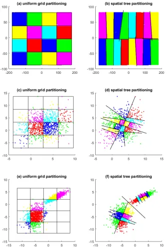
There are many existing methods to partition a large set of data into smaller pieces. The simplest spatial partitioning is a uniform grid partitioning that divides a domain into uniform grids and splits data accordingly (Park et al., 2011; Park and Huang, 2016). This is simple and effective if the data are uniformly distributed over a low dimensional space. However, if the input dimension is high, it would either generate too many regions or it would produce many sparse regions that contain very few or no observations, and the latter also happens when the data are non-uniformly distributed; see examples in Figure 2-(c) and Figure 2-(e). Shen et al. (2006) used a kd-tree for spatial partitioning of unevenly distributed data points in a high dimensional space. A kd-tree is a recursive partitioning scheme that recursively bisects the subspaces along one chosen data dimension at a time. Later, McFee and Lanckriet (2011) generalized it to the spatial tree. Starting with a level 0 space Ω(0)₁ equal to the entire regression domain, the spatial tree recursively bisects each of levelsspaces into two levels+ 1 spaces. Let Ω(_js)∈_Rd_{denote thejth region in the level}

sspace. It is bisected into two level s+ 1 spaces as

Ω(₂s_j+1)₋₁ ={x∈Ω(_js):vT_j,sx≤ν} and Ω₂(s_j+1)={x∈Ω_j(s) :vT_j,sx> ν}. (12) Each of Ω(₂s_j+1)₋₁ and Ω(₂s_j+1) will be further partitioned in the next level using the same

local data belonging to Ω(_js). For example, it can be the first principal component direction of the local data. The value forν is chosen so that Ω(₂s_j+1)₋₁ and Ω(₂s_j+1) have an equal number of observations. In this sense, the subregions at the same level are equally sized, which helps to level off the computation times of the local models. When the spatial tree is applied on data uniformly distributed over a rectangular domain, it produces a uniform grid partitioning; see examples in Figure 2-(b). The spatial tree is more effective than the grid partitioning when data is unevenly distributed; see examples in Figure 2-(d) and Figure 2-(f).

In this work, we use a spatial tree with the principal component (PC) direction forvj,s.

Bisecting a space along the PC direction has effects of minimizing the area of the interfacial boundaries in between the two bisected regions, so the number of the pseudo observations necessary for connecting the two regions can be minimized. The maximum level of the

recursive partitioning depends on the choice of K via smax = blog2Kc. The choices of K

and B will be discussed in the next section. Given B, the pseudo observations xk,l are

randomly generated from an uniform distribution over the intersection of the hyper-plane

vT_j,sx=ν and the level sregion Ω(_js).

4. Illustrative Example

To illustrate how patchwork kriging changes the model predictions (relative to a set of independent GP models over each region, with no continuity conditions imposed), we de-signed the following simple simulation study; we will present more comprehensive simulation comparisons and analyses in Section 5. We generated a dataset of 6,000 noisy observations

yi =f(xi) +i fori= 1, . . . ,6000,

from a zero-mean Gaussian process with an exponential covariance function of c(xi, xj) =

10 exp(−||xi−xj||2), where xi ∼Uniform(0,10) and i ∼ N(0,1) are independently

sam-pled, and f(xi) is simulated by the R package RandomField. Three hundred of the 6,000

observations were randomly selected as the training dataD, while the remaining 5,700 were

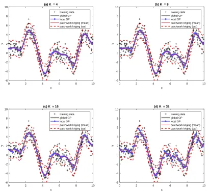
reserved for test data. Figure 3 illustrates how the patchwork kriging predictor changes for

differentK, relative to the global GP predictor and the regular local GP predictor with no

continuity conditions across regions. As the number of regions (K) increases, the regular

local GP predictor deviates more from the global GP predictor. The test prediction mean square error (MSE) for the regular local GP predictor at the 5,700 test locations is 0.0137

for K = 4, 0.0269 for K = 8, 0.0594 for K = 16, and 0.1268 for K = 32. In comparison,

patchwork kriging substantially improves the test MSE to 0.0072 for K = 4, 0.0123 for

K = 8, 0.0141 forK = 16, and 0.0301 forK = 32.

We also generated a synthetic dataset in 2-d using the R package RandomField, and we

denote this dataset by synthetic-2d. synthetic-2d consists of 8,000 noisy observations

from a zero-mean Gaussian process with the exponential covariance function ofc(xi, xj) =

10 exp(−||xi−xj||2),

yi =f(xi) +i fori= 1, . . . ,8000,

where xi ∼Uniform([0,6]×[0,6]) and i ∼ N(0,1) were independently sampled. We used

0 2 4 6 8 10

x

-6 -4 -2 0 2 4 6 8 10

y

(a) K = 4

training data global GP local GP

patchwork kriging (mean) patchwork kriging (var)

0 2 4 6 8 10

x

-6 -4 -2 0 2 4 6 8 10

y

(b) K = 8

training data global GP local GP

patchwork kriging (mean) patchwork kriging (var)

0 2 4 6 8 10

x

-6 -4 -2 0 2 4 6 8 10

y

(c) K = 16

training data global GP local GP

patchwork kriging (mean) patchwork kriging (var)

0 2 4 6 8 10

x

-6 -4 -2 0 2 4 6 8 10

y

(d) K = 32

training data global GP local GP

patchwork kriging (mean) patchwork kriging (var)

Figure 3: Example illustrating the patchwork kriging predictor, together with the global

GP predictor and the regular local GP predictor with no continuity constraints. K is the

number of local regions.

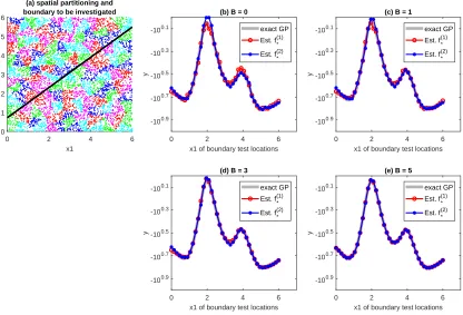
as B changes. We first partitioned the dataset into 128 local regions as shown in Figure

4-(a). For evaluation purposes, we considered test points that fell on the boundary cutting the entire regression domain into two (indicated by the black solid line in Figure 4-(a)), and sampled 201 test points uniformly over this boundary; the test locations do not coincide with the locations that pseudo observations placed. For each point, we get two mean predictions from the two local patchwork kriging models that straddle the boundary at that point.

We compared the two mean predictions to each other for different choices of B and also

compared them with the optimal global GP prediction, i.e., the prediction using the true GP covariance function and the entire dataset globally without spatial partitioning. Figure

4 shows the comparison. WhenB = 0, the two local models exhibited significant differences

0 2 4 6 x1 of boundary test locations -100.9

-100.7 -100.5 -100.3 -100.1

y

(b) B = 0

exact GP

Est. f(1)_*

Est. f(2)_*

0 2 4 6

x1 of boundary test locations -100.9

-100.7 -100.5 -100.3 -100.1

y

(c) B = 1

exact GP

Est. f(1)_*

Est. f(2)_*

0 2 4 6

x1 of boundary test locations -100.9

-100.7 -100.5 -100.3 -100.1

y

(d) B = 3

exact GP

Est. f(1)_*

Est. f(2)_*

0 2 4 6

x1 of boundary test locations -100.9

-100.7 -100.5 -100.3 -100.1

y

(e) B = 5

exact GP

Est. f(1)_*

Est. f(2)_*

0 2 4 6

x1 0

1 2 3 4 5 6

x2

(a) spatial partitioning and boundary to be investigated

Figure 4: Comparison of the patchwork kriging mean predictions of two local models over interfacial boundaries. Panel (a) shows how the entire regression domain was spatially partitioned into 128 local regions, which are distinguished by their colors. The black solid line cutting through the entire space is the interfacial boundary that we selected to study the behavior of the patchwork kriging at interfacial boundaries. Panels (b), (c), (d) and (e) compare the patchwork kriging mean predictions of the neighboring local models when

B = 0, 1, 3, and 5. In the panels, the horizontal axes represent the x1 coordinates of test

locations on the solid interfacial boundary line shown in panel (a). f∗(1) and f∗(2) denote

the mean predictions of the two local models on each side of the solid boundary line. As

B increases, the two local predictions converge to each other, and the converged values are

very close to the benchmark predictor achieved using the true GP model globally.

when B ≥5. The mean predictions were also very close to the exact GP predictions. The

similar results were observed in different simulated examples, which will be discussed in Section 5.

5. Evaluation with Simulated Examples

In this section, we use simulation datasets to understand how the patchwork kriging behaves

0 2 4 6 8 10 −8

−6 −4 −2 0 2 4 6 8 10

x

y

(a) short range

0 2 4 6 8 10

−5 0 5 10

x

y

(b) medium range

0 2 4 6 8 10

−12 −10 −8 −6 −4 −2 0 2

x

y

(c) long range

Figure 5: Illustrative Data with Short-range, Med-range and Long-range Covariances

5.1 Datasets and Evaluation Criteria

Simulation datasets are sampled from a Gaussian process with the squared exponential covariance function,

c(xi, xj) =τexp

−(xi−xj)

T_(x i−xj) 2ρ2

forxi, xj ∈Rd, (13)

where τ > 0 is the scale parameter, and ρ > 0 determines the range of covariance. We

randomly sampled 10,000 pairs of xi and yi. Each xi is uniformly from [0,10]d, and then

evaluate the sample covariance matrix with τ and ρ for the 10,000 sampled inputs, Cτ,ρ.

Allyi’s are jointly sampled fromN(0, σ2I+Cτ,ρ). We fixedτ = 10 andσ2= 1, but choseρ to 0.1 (short range), 1 (med range) or 10 (long range) to simulate datasets having different covariance ranges; see Figure 5 for illustrating simulated datasets for one dimensional input. In addition, the input dimension d was varied over {2,5,10,100}. In total, we considered

12 different combinations of different ρ and d values. For each combination, we drew 50

datasets, so there are 600 datasets in total.

For each of the datasets, we ran the patchwork kriging with different choices of K ∈

{16,32,64,128,256} and B ∈ {0,1,2,3,5,7,10,15,20,25}. For each run, we evaluate the computation time and prediction accuracy of patchwork kriging. For the prediction accu-racy, we first computed the predictive mean of the optimal GP predictor (i.e., using the true exponential covariance function) at test locations, and we used these optimal prediction values as a benchmark against which to judge the accuracy of the patchwork kriging predic-tions. One thousand test locations are uniformly sampled from the interior of local regions, denoted by{xt;t= 1, ..., TI}, and 200 additional test locations were uniformly sampled from the boundaries between local regions, which are denoted by {xt;t = TI+ 1, ..., TI +TB}.

Let µt denote the estimated posterior predictive mean at location xt, and let ˜µt denote

the benchmark predictive mean at the same location. We measure three performance met-rics for the mean predictions. The first two measures are the interior mean squared error (I-MSE) and the boundary mean squared error (B-MSE)

I-MSE = 1

TI TI

X

t=1

(˜µt−µt)2, and B-MSE = 1

TB TI+TB

X

t=TI+1

which measure the average accuracy of the mean prediction inside local regions and on the boundary of local regions. For each boundary point in {xt;t = TI + 1, ..., TI +TB}, we get two mean predictions from the two local patchwork kriging models that straddle the boundary at that point. In the B-MSE calculation, we took one of the two predictions following the rule: whenx∗ ∈Γkl, choose the prediction for f∗(k) ifk < l. Please note that

when a test location is at a corner where three or more local regions meet, we do have more than two predictions, which did not happen in all of our testing scenarios. We also evaluated the squared difference of the two mean predictions for each of 200 boundary points, and the mean squared mismatch (MSM) was defined as the average of the squared differences. We also measured the three performance metrics for the variance predictions, which were named ‘I-MSE(σ2)’, ‘B-MSE(σ2)’ and ‘MSM(σ2)’ respectively.

5.2 Analysis of the Outcomes and Choices of K and B

Figure 6 shows the I-MSE, B-MSE and MSM performance of the patchwork kriging for

different covariance ranges and different choices ofK and B when d= 100, and Appendix

C contains the plots of all six performance metrics for all simulation configurations. All of the performance metrics have shown the similar patterns:

• Covariance Ranges: All of the performance metrics became negligibly small for

medium-range and long-range covariances with largeB. This implies that the

patch-work kriging approximates the full GP very well for medium-range and longer-range covariances; please see Appendix for detailed plots. This result is opposite to our initial expectation that local-based approaches would have some deviations from the full GP for long-range covariances. As long as the underlying covariance is stationary, the proposed approach works well for long-range covariance cases.

• Effect ofB: All of the metrics decrease inB but does not change much forB above 8 for medium-range and long-range covariances. However, when the covariance range

is short, the improvement of the three metrics goes slower. This implies larger B is

required to achieve good accuracy for short-range covariances.

• Effect of K: All of the metrics increase in K when the other conditions are kept same. This is understandable, because the simulated data came from a stationary

process. However, the effect of K on the three metrics was relatively small when

B >7 and covariance ranges are medium or long. Since the computational complexity

of the proposed method decreases with increase of K, choosing a largeK withB >7

could be a computationally economic option with good prediction accuracy. See our

computation time analysis below for an additional discussion on the choices ofK and

B.

0 10 20 30 B 10-4 10-3 10-2 10-1 100 101 I-MSE d=100,short range K=16 K=32 K=64 K=128

0 10 20 30

B 10-4 10-3 10-2 10-1 100 101 I-MSE d=100,med range K=16 K=32 K=64 K=128

0 10 20 30

B 10-4 10-3 10-2 10-1 100 101 I-MSE d=100,long range K=16 K=32 K=64 K=128

0 10 20 30

B 10-4 10-3 10-2 10-1 100 101 B-MSE d=100,short range K=16 K=32 K=64 K=128

0 10 20 30

B 10-4 10-3 10-2 10-1 100 101 B-MSE d=100,med range K=16 K=32 K=64 K=128

0 10 20 30

B 10-4 10-3 10-2 10-1 100 101 B-MSE d=100,long range K=16 K=32 K=64 K=128

0 10 20 30

B 10-7 10-5 10-3 10-1 101 101.5 MSM d=100,short range K=16 K=32 K=64 K=128

0 10 20 30

B 10-7 10-5 10-3 10-1 101 101.5 MSM d=100,med range K=16 K=32 K=64 K=128

0 10 20 30

B 10-7 10-5 10-3 10-1 101 101.5 MSM d=100,long range K=16 K=32 K=64 K=128

Figure 6: Performance of Patchwork Kriging for Simulated Cases with 100 Input Dimen-sions.

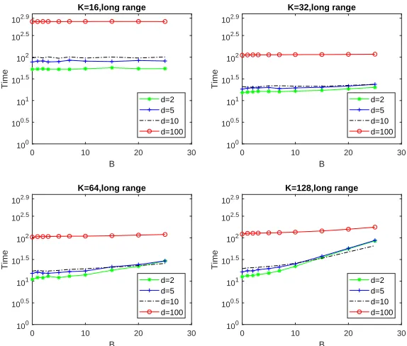
Figure 7 summarizes the total computation time of the patchwork kriging for different configuration.

• It appears that the input dimension is not a determining factor of the time if the input

dimension d ≤ 10, but for d > 10, it became a major factor to affect the time. As

we discussed in Section 3.3, the computational complexity of the patchwork kriging is

O(N3/K2 +d3_fB3K). When data are uniformly located over the regression domain,

df ∝dand the computation of the patchwork kriging is scaling proportionally tod3.

• Whend≤10, the deciding factor for the computation time wasK. In general, larger

0 10 20 30

B

100 100.5 101 101.5 102 102.5 102.9

Time

K=16,long range

d=2 d=5 d=10 d=100

0 10 20 30

B

100 100.5 101 101.5 102 102.5 102.9

Time

K=32,long range

d=2 d=5 d=10 d=100

0 10 20 30

B

100 100.5 101 101.5 102 102.5 102.9

Time

K=64,long range

d=2 d=5 d=10 d=100

0 10 20 30

B

100 100.5 101 101.5 102 102.5 102.9

Time

K=128,long range

d=2 d=5 d=10 d=100

Figure 7: Summary of Total Computation Times for Simulated Cases.

• With larger K, B becomes more influential to the total computation time. This

is due to the increase of the second term in the overall computational complexity,

O(N3/K2+d3_fB3K).

• To keep the total computation time lower, both of N/K and dfB should be kept

lower. On the other hand,N/K and dfB cannot be too small due to degradation of

prediction accuracy with a largeK and a small B.

Our numerical studies suggest to choose K so that N/K be in between 200 and 600 and

then choose B so that dfB is in between 15 and 400 to balance off the computation and

prediction accuracy; these were based on all of the simulation cases presented in this section as well as the six real data studies that will be presented in the next section. In order to

keep dfB ≤400 for efficient computation and B ≥7 for prediction accuracy, df ≤ 400/7.

Therefore, the proposed approach would benefit more for df ≤55. However, the proposed

approach still worked better than some existing approaches for the simulated cases with

d= 100; see the numerical results in Sections 5.3 and 5.4.

5.3 Comparison to a Global Approximation Method

We also used the simulated cases to compare the patchwork kriging to a global GP approx-imation method, the Fully Independent Training Conditional (FITC) algorithm (Snelson and Ghahramani, 2006, FITC). We decided to compare ours with the global GP approxi-mation method because we thought that the global GP approxiapproxi-mation would work better

when stationary covariances are used. For the patchwork kriging, we fixedB = 7 and varied

0 50 100 150 0 2 4 6 8 MSE time d=2,short range Ours FITC

0 50 100 150 200

0 2 4 6 8 10 MSE time d=5,short range Ours FITC

0 100 200 300

0 2 4 6 8 10 MSE time d=10,short range Ours FITC

0 500 1000 1500

0 2 4 6 8 10 MSE time d=100,short range Ours FITC

0 50 100 150

0 0.5 1 1.5 MSE time d=2,med range Ours FITC

0 50 100 150 200

0 0.5 1 1.5 2 2.5 MSE time d=5,med range Ours FITC

0 100 200 300

0 2 4 6 8 MSE time d=10,med range Ours FITC

0 500 1000 1500

0 2 4 6 8 MSE time d=100,med range Ours FITC

0 50 100 150 200

0 2 4 6 8x 10

−3 MSE time d=2,long range Ours FITC

0 50 100 150 200

0 0.002 0.004 0.006 0.008 0.01 MSE time d=5,long range Ours FITC

0 100 200 300

0 0.002 0.004 0.006 0.008 0.01 MSE time d=10,long range Ours FITC

0 500 1000 1500

0 0.5 1 1.5 MSE time d=100,long range Ours FITC

Figure 8: Comparison of Total Computation Times vs. MSE for Simulated Cases; triangles and stars represent the results of the patchwork kriging and FITC respectively.

the FITC performed better whend <10, but the patchwork kriging performed comparably

when d≥10.

The performance gap in between the FITC and the patchwork kriging can be explained by a more efficient computation of the patchwork kriging. Both of the FITC and patchwork kriging use pseudo inputs. Their accuracies depend on the total number of pseudo inputs

used. When Q pseudo inputs were applied for both of FITC and the patchwork kriging,

the computation of the FITC involves the inversion of a Q×Q dense matrix, while the

computation of the patchwork kriging involves the inversion of the sparse matrix of the same size that corresponds to equation (9). Therefore, when comparable computation times were invested, the patchwork kriging could place more pseudo inputs than the FITC, so it can give better accuracy. In addition, the locations of the pseudo inputs in the FITC need to be learned together with covariance hyperparameters, and the increase in the number of pseudo inputs would increase the computation time for hyperparameter learning.

5.4 Comparison to Local Approximation Methods

We also used the simulated cases to compare the patchwork kriging to two local GP approxi-mation methods, a robust Bayesian committee machine (Deisenroth and Ng, 2015, RBCM), and a partially independent conditional approach (Snelson and Ghahramani, 2007, PIC).

For the patchwork kriging, we fixed B = 7 and varied K ∈ {32,64,128}. For RBCM,

we used K ∈ {32,64,128}. For PIC, we used K ∈ {32,64,128} with the total number of

pseudo inputs fixed to 128. Figure 9 summarizes the comparison of MSE performance. The patchwork kriging performed very competitively for all simulated cases. The significant increase of computation time for the input dimension more than 10 was observed for all of the compared methods.

6. Evaluation with Real Data

In this section, we use five real datasets to evaluate the patchwork kriging and compare it with the state-of-the-art, including (Park and Huang, 2016, PGP), a Gaussian Markov random field approximation (Lindgren et al., 2011, GMRF), a robust Bayesian committee machine (Deisenroth and Ng, 2015, RBCM), and a partially independent conditional ap-proach (Snelson and Ghahramani, 2007, PIC). The comparison with one additional dataset is presented in Appendix D.

6.1 Datasets and Evaluation Criteria

We considered five real datasets: two spatial datasets in 2-d with different spatial distri-butions of observations, one additional spatial dataset with a very large data size, and three higher dimensional datasets, one with 9-dimension, another with 21-dimension and the other with 8-dimension.

The first spatial dataset,TCO.L2, 182,591 observations collected by the NIMBUS-7/TOMS

observa-0 20 40 time

0 1 2 3 4 5

MSE

d =2,short range

0 10 20

time 0

5 10

MSE

d =5,short range

0 10 20

time 0

1 2 3 4

MSE

d =10,short range

0 100 200

time 0

5 10

MSE

d =100,short range

0 20 40

time 0

0.5 1

MSE

d =2,med range

0 20 40

time 0

0.5 1

MSE

d =5,med range

0 20 40

time 0

0.5 1

MSE

d =10,med range

0 100 200

time 0

0.1 0.2 0.3 0.4

MSE

d =100,med range

0 10 20 30 40

time 0

0.005 0.01

MSE

d =2,long range

0 10 20 30 40

time 0

0.005 0.01 0.015 0.02

MSE

d =5,long range

0 10 20 30 40

time 0

0.005 0.01 0.015 0.02

MSE

d =10,long range

0 50 100 150 200

time 0

0.005 0.01 0.015 0.02

MSE

d =100,long range

Figure 9: Comparison of Total Computation Times vs. MSE for Simulated Cases; triangles, stars and circles represent data for the patchwork kriging, PIC and RBCM respectively. The number of circles are not always same because PIC could not produce outcomes for some simulated cases due to singularity in numerical inversion.

tions are uniformly spread over the range of the two predictors. The main analysis objective with this dataset is to predict the total column of ozone at unobserved locations.

The second dataset, ICETHICK, contains ice thickness measurements at 32,481 locations

on the western Antarctic ice sheet and is available at http://nsidc.org/. It has two

corresponding independent variable is the ice thickness measurement. The dataset has many sparse regions where there are very few observations. Regression analysis with this dataset would give the prediction of ice thickness at unobserved locations.

The third dataset,PROTEIN, has nine input variables that describe the tertiary structure

of proteins and one independent variable that describes the physiochemical property of

pro-teins. These data, which are available at https://archive.ics.uci.edu/ml/datasets,

consist of 45,730 observations. Like typical high dimensional datasets, the measurements are embedded on a low dimensional subspace of the entire domain. This dataset can be studied to relate the structure of a protein with the physiochemical property of the protein for predicting the property from the structure.

The fourth dataset, SARCOS, contains measurements from a seven degrees-of-freedom

SARCOS anthropomorphic robot arm. There are 21 predictors that describe the posi-tions, moving velocities and accelerations of seven joints of the robot arm, and the seven response variables are the corresponding torques at the seven joints. We only use the first

response variable for this numerical study. The dataset, which is available at http://www.

gaussianprocess.org/gpml/data/, contains 44,484 training observations and 4,449 test observations. The main objective of the regression analysis is to predict one of the joint torques in a robot arm when the values of the predictors are available.

The last dataset, FLIGHT, consists of 800,000 flight records randomly selected from

the database available at http://stat-computing.org/dataexpo/2009/. The same size

subset of the database was used as a benchmark dataset in literature (Hensman et al., 2013). Following the use in the literature, we used 8 predictors that include the age of the aircraft, distance that needs to be covered, airtime, departure time, arrival time, day of the week, day of the month and month, and the response variable is the arrival time delay. This dataset was studied to predict the flight delay time when the predictors are given.

Using the five datasets, we compare the computation time and prediction accuracy of patchwork kriging with other methods. We randomly split each dataset into a training set containing 90% of the total observations and a test set containing the remaining 10% of the observations. To compare the computational efficiency of methods, we measure total computation times. For comparison of prediction accuracy, we measure two performance metrics on the test data, denoted by {(xt, yt) : t = 1, . . . , T}, where T is the size of the

test set. Let µt and σt2 denote the estimated posterior predictive mean and variance at

location xt; when the testing location xt is in the domain boundary Γkl, we may have two

predictions, one forf(k)(xt) and the other for f(l)(xt), for which we choose one forf(k)(xt) if k < l. Please note that when a test location is at a corner where three or more local regions meet, we do have more than two predictions, which did not happen in all of our testing scenarios. We also evaluated the squared The first measure is the mean squared error (MSE)

MSE = 1

T

T

X

t=1

which measures the accuracy of the mean predictionµt at locationxt. The second measure is the negative log predictive density (NLPD)

NLPD = 1

T

T

X

t=1

(yt−µt)2

2σ2_t +

1

2log(2πσ

2

t)

. (16)

The NLPD quantifies the degree of fitness of the estimated predictive distributionN(µt, σt2) for the test data. These two criteria are used broadly in the GP regression literature. A smaller value of MSE or NLPD indicates better performance. All numerical experiments were performed on a desktop computer with Intel Xeon Processor W3520 and 6GB RAM. The comparison was made in between our method and the state-of-the-art previously listed. Note that the PGP and the GMRF approaches cannot be applied for more than two input dimensions, and so were only compared for the three spatial datasets. We tried two covariance functions, a squared exponential covariance function and an exponential covari-ance function. Note that the PIC method does not work with an exponential covaricovari-ance function because learning the pseudo inputs for the PIC method requires the derivative of a covariance function but an exponential covariance function is not differentiable. On the other hand, when an squared exponential covariance function is applied to the GMRF, the precision matrix construction is not straightforward. Therefore, we used a squared expo-nential covariance function for comparing the proposed approach with the PIC, RBCM, and PGP, while using an exponential covariance function for comparing it with the GMRF. For both of the cases, we assumed the same hyperparameters for local regions, and we used the entire training dataset to estimate the hyperparameters.

We chose and applied different partitioning methods for the compared methods. The choice of the partitioning schemes for the patchwork kriging and PGP is restrictive because every local region needs to be simply connected to minimize the area of the boundaries between local regions, so we used the spatial tree. The GMRF comes with a mesh generation scheme instead of a partitioning scheme, and following the suggestion by the GMRF’s authors, we used the voronoi-tessellation of training points for the mesh generation. We tested the k-means clustering and the spatial tree for PIC and RBCM, but the choice did not make much difference in their performance. The results reported in this paper were the ones with the k-means clustering.

We tried different numbers of the local regions that partition an input domain, and the numbers of the local regions were ranged so that the numbers of observations per local region would be approximately in between 80 and 600 for the proposed approach. The numbers were similarly ranged for the other compared methods with some variations to have the computation times of all the compared methods comparable; note that we like to compare the prediction accuracies of the methods when the computation times spent are comparable. For patchwork kriging, the locations of pseudo observation were selected using the rule described in Section 3.4. For PIC, the locations were regarded as hyperparameters and were optimized using marginal likelihood maximization.

6.2 Example 1: TCO.L2 Dataset

0 200 400 600 800 1000 1200 1400 1600 1800 40

60 80 100 120 140 160

computation time (sec)

MSE

Time v.s. MSE for TCO.L2 Dataset

0 200 400 600 800 1000 1200 1400 1600 1800 3.3

3.4 3.5 3.6 3.7 3.8 3.9 4 4.1 4.2

computation time (sec)

NLPD

Time v.s. NLPD for TCO.L2 Dataset PIC

PGP Our Method

PIC PGP Our Method

0 1000 2000 3000 4000 5000 6000 45

50 55 60 65 70 75 80 85 90

computation time (sec)

MSE

Time v.s. MSE for TCO.L2 Dataset

0 1000 2000 3000 4000 5000 6000 3

3.5 4 4.5 5 5.5

computation time (sec)

NLPD

Time v.s. NLPD for TCO.L2 Dataset PGP

Our Method GMRF

PGP Our Method GMRF

Figure 10: Prediction accuracy versus total computation time for theTCO.L2data.

The prediction accuracy of the PGP did not depend on the number of local regions K, so

we fixed K = 623, while the number of finite element meshes per local region was

var-ied from 5 to 25 with step size 5. For RBCM, we varvar-ied the number of local experts

K ∈ {100,150,200,250,300,600}. For PIC, K was varied over {100,200,300,400,600}, and the total number of pseudo inputs was also varied over{50,70,80,100,150,200,300}.

Figure 10 shows the main results. The shortest computation time of RBCM (2319 seconds) was much longer than the longest time of the other compared methods, while its MSE was not competitive as well. Therefore we did not plot its results in the figure. For both of the square exponential and the exponential covariance functions, our approach and the PGP approach had comparable MSE. However, our approach significantly outperformed the PGP and PIC approaches in terms of the NLPD. This implies that our approach provides more accurate variance estimations.

6.3 Example 2: ICETHICK Dataset

One characteristic of this dataset is the presence of many spatial voids where there are

no or very little data points. For patchwork kriging, we varied B ∈ {3,5,7} and K ∈

{64,128,256,512,1024}. For the PGP, we used K = 47, while the number of finite

0 50 100 150 200 250 300 350 400 450 103

104

105 106 107 108 109

computation time (sec)

MSE

Time v.s. MSE for ICETHICK Dataset

0 50 100 150 200 250 300 350 400 450 100

101

102 103 104 105 106

computation time (sec)

NLPD

Time v.s. NLPD for ICETHICK Dataset PIC

RBCM PGP Our Method

PIC RBCM PGP Our Method

50 100 150 200 250 300 350 400 0

5 10 15x 10

4

computation time (sec)

MSE

Time v.s. MSE for ICETHICK Dataset

50 100 150 200 250 300 350 400 5.4

5.6 5.8 6 6.2 6.4 6.6 6.8 7 7.2 7.4

computation time (sec)

NLPD

Time v.s. NLPD for ICETHICK Dataset PGP

Our Method GMRF

PGP Our Method GMRF

Figure 11: Prediction accuracy versus total computation time for the ICETHICK data. A

squared exponential covariance function was used for the results in the top panel, while an exponential covariance function was used for the results in the bottom panel.

varied the number of local experts K ∈ {50,100,150,200,250,300}. For PIC, M was

var-ied over {50,100,150,200}, and the total number of pseudo inputs was also varied over

{50,100,150,200,300,400,500,600,700}.

Figure 11 compares the MSE and NLPD performance of the methods. Again, the PGP approach and the proposed approach outperformed the other methods, and the proposed approach achieved the best accuracy with much less computation time than the PGP ap-proach. In addition, the proposed approach uniformly outperformed the other methods in terms of the NLPD. In other words, the proposed approach gives a predictive distribution that better fits the test data.

6.4 Example 3: PROTEIN Dataset

Different from the previous datasets, this dataset features nine input variables. We will use this dataset to see how the proposed approach works for input dimension more than two. For the patchwork kriging, we varied B ∈ {2,3,4} and varied K ∈ {64,128,256}; we have

not included the results for larger B because a larger B increased the computation times

0 500 1000 1500 2000 2500

101

102

103

104

105

computation time (sec)

MSE

Time v.s. MSE for PROTEIN Dataset

0 100 200 300 400 500 600 700

101.16

101.18

101.2

101.22

101.24

101.26

computation time (sec)

MSE

Time v.s. MSE for PROTEIN Dataset

0 100 200 300 400 500 600 700 0

5 10 15 20 25 30

computation time (sec)

NLPD

Time v.s. NLPD for PROTEIN Dataset

0 500 1000 1500 2000 2500 0

5 10 15 20 25 30

computation time (sec)

NLPD

Time v.s. NLPD for PROTEIN Dataset

PIC RBCM Our Method

PIC RBCM Our Method

PIC Our Method

PIC Our Method

Figure 12: Prediction accuracy versus total computation time for the PROTEIN data. The

upper panel compares all three methods. Since the performance of the PIC and our method was very close, the bottom panel provides a closer look of the PIC and our method.

PGP and GMRF approaches do not work with input dimensions more than two, and so were not included in this comparison. For RBCM, we varied the number of local experts

K ∈ {100,150,200,250,300}. For PIC,K was varied over{100,150,200,250,300}, and the total number of pseudo inputs (M) was also varied over {100,150,200,250,300}. In this comparison, we used a squared exponential covariance function for all three methods.

Figure 12 shows the main results. For this dataset, the PIC approach outperformed our method in terms of the MSE performance, providing more accurate mean predictions. On the other hand, our method provided better NLPD performance, which implies that the predictive distribution estimated by our method was better fit to test data than that of the PIC. Figure 13 compares the predictive distributions estimated by the two methods. In the

figure, the predicted mean±1.5 predicted standard deviations was plotted for 100 randomly

0 10 20 30 40 50 60 70 80 90 100 −20

0 20 40

(a) Our method

0 10 20 30 40 50 60 70 80 90 100

−20 0 20 40

(b) PIC

mean test data

mean± 1.5 std. dev.

mean test data

mean± 1.5 std. dev.

Figure 13: Comparison of the predictive distributions estimated by our method and by the

PIC method for thePROTEIN data.

normal random variable within±1.5σ is 86.64%. Clearly, our method provides a better fit

to the test data.

6.5 Example 4: SARCOS Dataset

This dataset has 21 input variables. For patchwork kriging, we varied B ∈ {3,5,7}, and

we varied K ∈ {128,256}. Again, the PGP and GMRF approaches do not work with high

dimensional inputs, and so were not included in this comparison. For the RBCM approach, we varied the number of local expertsK∈ {100,150,200,250,300}. For PIC,K was varied over {100,150,200,250,300}, and the total number of pseudo inputs (M) was also varied over{100,150,200,250,300}. In this comparison, we used a squared exponential covariance function for all three methods.

0 500 1000 1500 2000 2500 3000

computation time (sec)

10-2

10-1 100 101 102

MSE

Time v.s. MSE for SARCOS Dataset

PIC RBCM Our Method

0 500 1000 1500 2000 2500 3000

computation time (sec)

2 3 4 5 6 7

NLPD

Time v.s. NLPD for SARCOS Dataset

RBCM Our Method

Figure 14: Prediction accuracy versus total computation time for the SARCOS data. A

squared exponential covariance function was used. The PIC approach produced negative predictive variances, so its NLPD could not be computed. In the MSE plot, four triangles are supposed to show up. However, two of the four triangles are very closely located, so it looks like that there are only 3 triangles.

Methods MSE NLPD Computation Time (seconds)

Ours 1188.4 4.8917 11729

RBCM 9790.2 10.5630 13218

PIC (M = 1000) 1494.8 5.0742 1624

PIC (M = 1500) 1492.7 5.0731 2094

Table 1: Comparison of MSE and NLPD performance forFlight DelaysDataset.

6.6 Example 5: Flight Delays Dataset

This dataset has 800,000 records and eight input variables. For this dataset, due to memory limitation of our testing environment, we could not try various cases with different choices

of tuning parameters. For patchwork kriging, we fixed K = 1024 and B = 5. For the

RBCM, we set the number of local expertsK = 1024. For PIC, we setK = 1024, and the

total number of pseudo inputs (M) was chosen to 1000 or 1500, and the further increase

of M gave an out-of-memory error in our testing environment. Note that PIC requires to

precompute K dense covariance matrices of size N/K×M, which could be very large for

this scale of N and M.

Table 1 summarizes the MSE and NLPD performance of our method, RBCM and PIC. The proposed approach gave a better MSE than the RBCM with less use of computation time. PIC showed very competitive computation performance, but its MSE was not as good

as the MSE of our method. The increase ofM could improve the PIC’s MSE performance,