The Thirty-Third AAAI Conference on Artificial Intelligence (AAAI-19)
Data Fine-Tuning
Saheb Chhabra, Puspita Majumdar, Mayank Vatsa, Richa Singh
IIIT-Delhi, India{sahebc, pushpitam, mayank, rsingh}@iiitd.ac.in
Abstract
In real-world applications, commercial off-the-shelf systems are utilized for performing automated facial analysis includ-ing face recognition, emotion recognition, and attribute pre-diction. However, a majority of these commercial systems act as black boxes due to the inaccessibility of the model param-eters which makes it challenging to fine-tune the models for specific applications. Stimulated by the advances in adversar-ial perturbations, this research proposes the concept of Data Fine-tuning to improve the classification accuracy of a given model without changing the parameters of the model. This is accomplished by modeling it as data (image) perturbation problem. A small amount of “noise” is added to the input with the objective of minimizing the classification loss without af-fecting the (visual) appearance. Experiments performed on three publicly available datasets LFW, CelebA, and MUCT, demonstrate the effectiveness of the proposed concept.
Introduction
With the advancements in machine learning (specifically deep learning), ready to use Commercial Off-The-Shelf (COTS) systems are available for automated face analy-sis, such as face recognition (Ding and Tao 2018), emotion recognition (Fan et al. 2016), and attribute prediction (Hand, Castillo, and Chellappa 2018). However, often times the de-tails of the model are not released which makes it difficult to update it for any other task or datasets. This renders the model’s effectiveness as a black-box model only. To illus-trate this, letXbe the input data for a model with weights
Wand biasb. This model can be expressed as:
φ(WX+b) (1)
If the source of the model is available, model fine-tuning is used to update the parameters. However, as mentioned above, in black box scenarios, the model parameters,Wand
bcannot be modified, as the user does not have access to the model.
“Can we enhance the performance of a black-box system for a given dataset?” To answer this question, in this re-search, we present a novel concept termed as Data Fine-tuning (DFT), wherein the input data is adjusted corre-sponding to the model’s unseen decision boundary. To the
Copyright c2019, Association for the Advancement of Artificial
Intelligence (www.aaai.org). All rights reserved.
X-axis
Y
-a
xis
Class 1
Class 2
Model Fine-tuning
(a)
Pre-trained model’s decision boundary
Fine-tuned model’s decision boundary Data
Fine-tuning
X-axis
Y
-a
xis
Class 1
Class 2
(c)
X-axis
Class 1
Class 2
(b)
Y
-a
xis 𝜙(W’X+b’) 𝜙(WX+b)
𝜙(WZ+b)
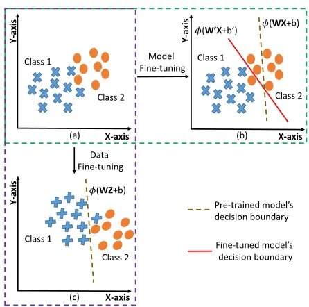
Figure 1: Illustration of model tuning and data fine-tuning: (a) represents the data distribution with two classes. (b) represents Model Fine-tuning where the model’s deci-sion boundary shifts corresponding to the input data, and (c) represents Data Fine-tuning where the input data shifts corresponding to model’s decision boundary (best viewed in color).
best of our knowledge, this is the first work towards data fine-tuning to enhance the performance of a given black box system. As shown in Figure 1, the proposed data fine-tuning adjusts the input dataXwhereas, in the model fine-tuning approach (MFT), the parameters (W,b) are adjusted for op-timal classification.
Mathematically, model fine-tuning is:
φ(WX+b)−−→MFT φ(W0X+b0) (2)
and data fine-tuning can be written as:
King penguin Perturbation chihuahua
Sophia Perturbation Sophia
Female, White
Male, Black
Attack on Deep learning models
Attribute Prediction Model
Classification accuracy x %
Attribute Prediction Model
Classification accuracy (x + y) %
Perturbation
Privacy Preservation (a)
(b)
Proposed: Data Fine-tuning
(c)
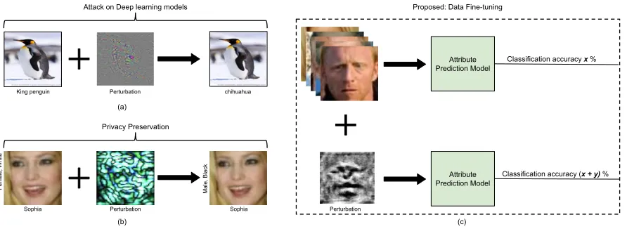
Figure 2: Comparing the concept of adversarial perturbation with data fine-tuning. (a) Adversarial perturbation: shows the application of perturbation in attacking deep learning models (Xie et al. 2017). (b) Privacy preservation: perturbation can be used to anonymize the attributes by preserving the identity of the input image (Chhabra et al. 2018). (c) Data Fine-tuning: illustrates the proposed application of perturbation in enhancing the performance of a model (best viewed in color).
where, MFT and DFT are model fine-tuning1and data
fine-tuning, respectively. (W0,b0) are the parameters after MFT
andZis the perturbed version of input Xafter data fine-tuning.
In this research, the proposed data fine-tuning is achieved using adversarial perturbation. For this purpose, samples in the training data are uniformly perturbed and the model is trained iteratively on this perturbed training data to mini-mize classification loss. After each iteration, optimization is performed over the perturbation noise and added to the training data. At the end of the training, a single uniform perturbation is learned corresponding to a dataset. As a case study, the proposed algorithm is evaluated for facial attribute classification. It learns a single universal perturbation for a given dataset to improve facial attribute classification while preserving the visual appearance of the images. Experiments are performed on three publicly available datasets and re-sults showcase enhanced performance of black box systems using data fine-tuning.
Related Work
In the literature, perturbation is studied from two perspec-tives: (i) privacy preservation and (ii) attacks on deep learn-ing models. For privacy preservation, several techniques uti-lizing data perturbation are proposed. (Jain and Bhandare 2011) proposed min max normalization method to perturb data before using in data mining applications. (Last et al. 2014) proposed a data publishing method using NSVDist. Using this method, the sensitive attributes of the data are published as the frequency distributions. Recently, (Chhabra et al. 2018) proposed an algorithm to anonymize multi-ple facial attributes in an input image while preserving the identity using adversarial perturbation. (Li and Zhou
1
Various data augmentation techniques have also been used for model fine-tuning (Salamon and Bello 2017; Um et al. 2017; Wu et al. 2018)
2018) proposed Random Linear Transformation with Con-densed Information-Support Vector Machine to convert the condensed information to another random vector space to achieve safe and efficient data classification.
(Szegedy et al. 2013) demonstrated that application of im-perceptible perturbation could lead to the misclassification of an image. (Papernot et al. 2016) created an adversarial attack by restrictingl0-norm of the perturbation where only
a few pixels of an image are modified to fool the classifier. (Carlini and Wagner 2017) introduced three adversarial at-tacks and showed the failure of defensive distillation (Carlini and Wagner 2016) for targeted networks. By adding pertur-bation, (Kurakin, Goodfellow, and Bengio 2016) replaced the original label of the image with the label of least likely predicted class by the classifier. This lead to the poor classi-fication accuracy of Inception v3. (Su, Vargas, and Kouichi 2017) proposed a one-pixel attack in which three networks are fooled by changing one pixel per image. Universal ad-versarial perturbation proposed by (Moosavi-Dezfooli et al. 2017) can fool a network when applied to any image. This overcomes the limitation of computing perturbation on every image. (Goswami et al. 2018) proposed a technique for auto-matic detection of adversarial attacks by using the abnormal filter response from the hidden layer of the deep neural net-work. Further, a novel technique of selective dropout is pro-posed to mitigate the adversarial attacks. (Goel et al. 2018) developed SmartBox toolbox for detection and mitigation of adversarial attacks against face recognition.
𝑿 = {𝑿𝟏, 𝑿𝟐, . . 𝑿𝒎} 𝑵
𝒁 = {𝒁𝟏, 𝒁𝟐, . . 𝒁𝒎}
Attribute Prediction
𝒁 Minimize Loss
𝓕(𝒚, 𝑃(𝑨|𝒁)) 𝑃(𝑨|𝒁)
True Labels
𝒚
Optimize over variable 𝑵
(a)
(b)
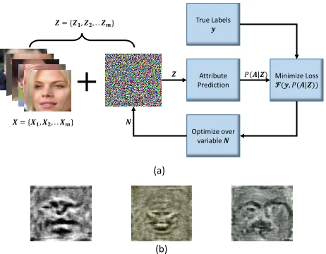
Figure 3: (a) Block diagram illustrating the steps of the pro-posed algorithm. In the first step, perturbation is initialized with zero image and added to the original training data. In the next step, perturbed training data is given as input to the (attribute prediction) model followed by the computation of loss. After that, optimization is performed over perturba-tion and added to the training data. (b) Some samples of the learned perturbation using the proposed algorithm. The first two visualizations correspond to the perturbation learned for ‘Smiling’ attribute of LFW and CelebA datasets, respec-tively. The third visualization corresponds to the ‘Gender’ attribute of the MUCT dataset (best viewed in color).
Proposed Approach: Data Fine-tuning
Considering a black-box system as a pre-trained model, the problem statement can be defined as “given the dataset Dand pre-trained modelM, learn a perturbation vectorNsuch that adding noiseNtoDimproves the performance of the model M on D”. There are two important considerations while performing data fine-tuning:
1. To learn a single universal perturbation noise for a given dataset.
2. The visual appearance of the image should be preserved after performing data fine-tuning.
The block diagram illustrating the steps involved in the proposed algorithm is shown in Figure 3. The optimiza-tion process for data fine-tuning using adversarial perturba-tion with applicaperturba-tions to facial attribute classificaperturba-tion is dis-cussed below. This same approach can be extended for other classification models.
Given the original training setXwithmnumber of im-ages where each image, Xk has pixel values in the range {0,1}, i.e.,Xk ∈ [0,1]. LetZ be the perturbed training set generated by adding model specific perturbation noise
Nsuch that the pixel values of each output perturbed image
Zkranges between0to1, i.e.,Zk∈[0,1]. Mathematically, it is written as:
Zk=f(Xk+N) (4)
such that f(Xk+N)∈[0,1]
where,f(.)represents the function to transform an image in the range of 0 to 1. In order to satisfy the above constraint, inspired by (Carlini and Wagner 2017), the following func-tion is used:
Zk=
1
2(tanh(Xk+N) + 1) (5) For each imageXkthere arennumber of attributes in the attribute set A, where each attribute Ai has Cj number of classes. For example, ‘Gender’ attribute has two classes namely {Male, Female} while ‘Expression’ attribute has three classes namely{Happy, Sad, Anger}. Mathematically, it is written as:
A={A1(C1),A2(C2), ...An(Cn)} (6) The pre-trained attribute prediction model for attributeAi is represented as φAi(Xk,W, b), where W is the weight matrix andb is the bias. The output attribute score of any imageXkis written as:
P(Ai|Xk) =φAi(Xk,W, b) (7)
where, P(Ai|Xk) represents the output attribute score of the input imageXkfor attributeAi. In order to perform data fine-tuning, perturbationNis added to each input imageXk to get the output perturbed imageZkusing Equation 5. Here,
N is the perturbation variable to be optimized. The output attribute score of the perturbed imageZkis represented as:
P(Ai|Zk) =φAi(Zk,W, b) (8)
In order to enhance the model’s performance for attribute
Ai, the distance between the true class and attribute pre-dicted score of the perturbed image is minimized which is expressed as:
min
N F(yi,k, P(Ai|Zk)) (9) where, F(., .)represents the function to minimize the dis-tance between the true class and the predicted class. yi,k represents the true class of attribute Ai in one hot encod-ing form of the original imageXk. To preserve the visual appearance of the output perturbed imageZk, the distance between original imageXk and the perturbed imageZk is minimized. Thus, the above equation is updated as:
min
N F(yi,k, P(Ai|Zk)) +H(Xk,Zk) (10) where,Hrepresents the distance metric to minimize the dis-tance betweenXkandZk. In this research, Euclidean dis-tance metric is used to preserve the visual appearance of the image. Therefore,
min
N F(yi,k, P(Ai|Zk)) +||Xk−Zk||
2
F (11)
Since the output class score ranges between 0 and 1, the objective function in Equation (9) is formulated as:
F(yi, P(Ai|Z)) = 1
m
m X
k=1
max(0,1−yTi,kP(Ai|Zk))
Dataset: 𝑫𝟏 Class 2 Class 1 (a) X-axis Y -a xi
s Input Image
Space Class 2 Class 1 (b) X-axis Y -a xi
s Output Class
Scores
Training on Dataset 𝑫𝟏
Attribute Prediction Model
Class 1 Class 2 Dataset: 𝑿
(c) X-axis Input Image Space Class 1 Class 2 (d) X-axis Output Class Scores Class 1 Class 2 (f) X-axis Output Class Scores
Class 1 Class 2
(e) X-axis
Input Image Space
Fine tuned Dataset: 𝒁
Pre-trained Attribute Prediction Model Pre-trained Attribute Prediction Model Add Perturbation Data fine-tuning Y -a xi s Y -a xi s Y -a xi s Y -a xi s
𝜙(W𝑫𝟏+b) 𝜙(WX+b) 𝜙(WZ+b)
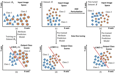
Figure 4: Illustration of the proposed DFT algorithm. Fig-ure (a)-(b) represents the training of attribute prediction model using datasetD1. (c)-(d) shows the performance of the trained attribute prediction model on dataset X. (e)-(f) shows the performance of the fine-tuned dataset Z by adding perturbation on trained attribute prediction model. (Best viewed in color).
where,i ∈ {1, ..., n}, and the termyT
i,kP(Ai|Zk)outputs the attribute score of the true class. As the above function F(yi, P(Ai|Z))is to be minimized, the termmax(0,1−
yTi,kP(Ai|Zk)) enforces the output attribute score of the true class of the perturbed imageZktowards one.
Figure 4 illustrates the proposed algorithm with an exam-ple. LetD1be the dataset with two classes in the input im-age space (Figure 4(a)) and it is used to train a model,M1.
ModelM1computes the decision boundary and projects the
output class scores corresponding to the input dataD1 as shown in Figure 4(b). It is observed that the output class scores are well separated across the decision boundary for the datasetD1. Now, the pre-trained modelM1is used for
projecting the input datasetX(Figure 4(c)). The decision boundary of the modelM1remains fixed. The projected
out-put class scores of the inout-put dataXare shown in Figure 4(d). It is observed that most of the data points of both the classes are projected on the same side of the decision boundary re-sulting in a high classification error. This is due to the change in the data distribution of the input datasetX. To overcome this problem, input datasetX is fine-tuned by adding per-turbation noise. Figure 4(e) shows the fine-tuned datasetZ
that is given as input to the modelM1. The projection of the
fine-tuned datasetZis shown in Figure 4(f). On comparing the output class scores of the projection of input dataXand fine-tuned data Z, it is observed that several misclassified samples fromXare correctly classified with the fine-tuned datasetZ.
Datasets Protocol and Experimental Details
The proposed algorithm is evaluated on three publicly avail-able datasets for facial attribute classification: LFW (Huang et al. 2008), CelebA (Liu et al. 2015), and MUCT (Mil-borrow, Morkel, and Nicolls 2010). A comparison has also been performed between Data tuning and ModelFine-Table 1: Details of the experiments to show the efficacy of the proposed data fine-tuning for facial attribute classifica-tion.
Experiment Data Fine-tuning Model Training
Attribute Database Database
Black Box Data Fine-tuning: Intra Dataset Gender MUCT MUCT LFW LFW CelebA CelebA Smiling, Bushy Eyebrows Pale Skin LFW LFW Smiling, Attractive,
Wearing Lipstick CelebA CelebA
Black Box Data Fine-tuning: Inter Dataset
Gender
MUCT LFW, CelebA LFW MUCT, CelebA CelebA MUCT, LFW Smiling, Bushy
Eyebrows, Pale Skin
LFW CelebA
Smiling, Attractive,
Wearing Lipstick CelebA LFW
tuning. The details of each dataset and its protocol are de-scribed below :
LFW dataset consists of 13,133 images of 5,749 sub-jects. Total 73 attributes are annotated with intensity values for each image. The attributes are binarized by considering positive intensity values as attribute present with label 1 and negative intensity values as attribute absent with label 0. The dataset is partitioned into 60% training set, 20% validation set, and 20% testing set.
CelebA datasetconsists of 202,599 face images of more than 10,000 celebrities. For each image, 40 binary attributes are annotated such as Male, Smiling, and Bushy Eyebrows. Standard pre-defined protocol is followed for experiments and the dataset is partitioned into 162,770 images in the training set, 19,867 into validation set, and 19,962 images in the testing set.
MUCT datasetconsists of 3,755 images of 276 subjects out of which 131 are male and 146 are female. Viola-Jones face detector is applied on all the images, and the detector failed to detect 49 face images. Therefore, only 3,706 im-ages are considered for further processing. These imim-ages are further partitioned into 60% training set, 20% validation set, and 20% testing set corresponding to each class.
To evaluate the performance of data fine-tuning, two ex-periments are performed, (i) Black Box Data Fine-tuning: Intra Dataset and (ii) Black Box Data Fine-tuning: Inter Dataset. Both the experiments are performed on all the three datasets. Classification performance of the attributes is en-hanced corresponding to the attribute classification model. To train the attribute classification model, pre-trained VG-GFace (Parkhi et al. 2015) + NNET is used. Experimental details are also shown in Table 1.
Implementation Details
The implementation details of training attribute classifica-tion model, perturbaclassifica-tion learning, and model fine-tuning are discussed below.
Misclassified: Before DFT
Correctly
classified: After
DFT
Smiling
attribute Bushy Eyebrows attribute
Pale Skin attribute
Not Smiling
Smiling Smiling
Not Smiling
Not Bushy Eyebrows
Bushy Eyebrows Bushy Eyebrows
Not Bushy Eyebrows
Not Pale Skin
Pale Skin Pale Skin
Not Pale Skin
Figure 5: Misclassified samples that are correctly classified after data fine-tuning. First row shows the images misclassified before data fine-tuning while the second row represents their correct classification after data fine-tuning. The first block of images correspond to the ‘Smiling’ attribute, second block corresponds to ‘Bushy Eyebrows’, while the third block corresponds to ‘Pale Skin’ of the LFW dataset. (Best viewed in color).
Table 2: Classification accuracy (in %) of before and af-ter Data Fine-tuning(DFT) for ‘Gender’ attribute on LFW, CelebA, and MUCT datasets.
Before DFT After DFT
LFW 87.94 91.17
CelebA 82.13 83.08
MUCT 91.67 94.31
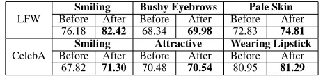
Table 3: Classification accuracy (in %) before and after per-forming data fine-tuning for three attributes on the LFW and CelebA datasets.
LFW
Smiling Bushy Eyebrows Pale Skin
Before After Before After Before After
76.18 82.42 68.34 69.98 72.83 74.81
CelebA
Smiling Attractive Wearing Lipstick
Before After Before After Before After
67.82 71.30 70.48 70.54 80.95 81.29
512 dimensions. Each model is trained for 20 epochs with Adam optimizer, and learning rate is set to 0.005.
Perturbation Learning: To learn the perturbation for a given dataset, learning rate is set to 0.001 and the batch size is 800. The number of iterations used for processing each batch is 16, and the number of epochs is 5.
Model Fine-tuning:To fine-tune the attribute classification model, Adam optimizer is used with learning rate set to 0.005. The model is trained for 20 epochs.
Performance Evaluation
The performance of the proposed algorithm is evaluated forBlack Box Data Fine-tuning: Intra Dataset Experiment, where the dataset used for data fine-tuning is same on which the pre-trained model is trained. On the other hand, inBlack Box Data Fine-tuning: Inter Dataset Experiment, the train-ing data used to perform data fine-tuntrain-ing is different from the training data used to train the pre-trained model.
Score
P
robab
ility
Dis
trib
u
tion
Figure 6: Smiling attribute score distribution pertaining to before and after performing data fine-tuning on the LFW dataset. The left graph represents the score distribution be-fore data fine-tuning and right graph represents the score dis-tribution after data fine-tuning. (Best viewed in color).
Black Box Data Fine-tuning: Intra Dataset
Experiment
The proposed algorithm is evaluated on LFW, CelebA, and MUCT datasets for enhancing the performance of black box models. ‘Gender’ is the common attribute among all three datasets. Table 2 shows the classification accuracy pertain-ing to before and after data fine-tunpertain-ing for ‘Gender’ at-tribute. For all three datasets, the classification accuracy im-proves by 1% to 3% using data fine-tuning. Specifically, the classification accuracy increases by 2.64% for MUCT dataset whereas, for LFW dataset, the accuracy increases by 3.21%.
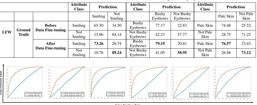
Table 4: Confusion matrix of the LFW dataset for three attributes: ‘Smiling’, ‘Bushy Eyebrows’, ‘Pale Skin’. Attribute
Class Prediction
Attribute
Class Prediction
Attribute
Class Prediction
Smiling SmilingNot EyebrowsBushy Not BushyEyebrows Pale Skin Not PaleSkin
LFW Ground
Truth
Before Data Fine-tuning
Smiling 65.50 34.50 Bushy
Eyebrows 77.17 22.83 Pale Skin 74.48 25.52
Not
Smiling 15.86 84.14
Not Bushy
Eyebrows 42.23 57.77
Not Pale
Skin 28.75 71.25
After Data Fine-tuning
Smiling 73.26 26.74 EyebrowsBushy 79.19 20.81 Pale Skin 76.57 23.43
Not
Smiling 10.76 89.24
Not Bushy
Eyebrows 41.05 58.95
Not Pale
Skin 26.88 73.12
False Positive Rate
Tr
ue
Posit
iv
e R
at
e
Figure 7: ROC plots showing before and after data fine-tuning results of Black box Data Fine-tuning: Inter Dataset Experiment. First three ROC curves shows the result on the LFW dataset using a model trained on the CelebA dataset. Last three ROC curves shows the result on the CelebA dataset using a model trained on the LFW dataset (best viewed in color).
Table 5: Classification accuracy(%) of Black box Data Fine-tuning: Inter Dataset experiment for ‘Gender’ attribute on the MUCT, LFW, and CelebA datasets.
Dataset used to train the model
MUCT LFW CelebA
Before After Before After Before After
Dataset
MUCT - - 57.84 83.65 80.27 92.84 LFW 63.09 80.45 - - 56.01 86.33 CelebA 49.14 74.73 67.53 76.59 -
-Figure 5 shows some misclassified samples of LFW dataset corresponding to ‘Smiling’, ‘Bushy Eyebrows’, and ‘Pale Skin’ attributes that are correctly classified after data fine-tuning. It is also observed that the visual appearance of the images is preserved. The score distribution of ‘Smiling’ attribute, before and after data fine-tuning is shown in Fig-ure 6. It is observed that the overlapping region between both the classes is reduced, and the confidence of predict-ing the true class scores is increased after data fine-tunpredict-ing. The confusion matrix corresponding to the three attributes of the LFW dataset is shown in Table 4 which indicates that the True Positive Rate (TPR) and True Negative Rate (TNR) is improved for all three attributes. For instance, the TPR of ‘Smiling’ attribute is increased by approximately 8% and TNR is increased by approximately 5% showcasing the effi-cacy of the proposed technique.
Black box Data Fine-tuning: Inter Dataset
Experiment
This experiment is performed considering the real world sce-nario associated with Commercial off-the-shelf (COTS) sys-tems where the training data distribution of the system is
un-Table 6: Classification accuracy(%) of Black box Data Fine-tuning: Inter Dataset experiment.
Pre-trained Model trained on CelebA
LFW
Smiling Bushy Eyebrows Pale Skin
Before After Before After Before After
55.29 78.61 45.40 68.91 56.62 84.21
Pre-trained Model trained on LFW
CelebA
Smiling Attractive Wearing Lipstick
Before After Before After Before After
49.07 66.97 49.71 66.60 60.25 77.15
fine-B
ef
o
re
Da
ta
Fi
n
e-tu
n
ing
Af
ter
Da
ta
Fi
n
e-tu
n
ing
Score
P
robab
ility
Dis
trib
u
tion
Figure 8: Score distributions pertaining to before and after performing data fine-tuning. Top three graphs from the left represent the distribution ofthe LFW dataset predicted using a model trained on the CelebA dataset. Bottom three graphs from the left represent its corresponding distribution after data fine-tuning. Similarly top three graphs from the right represent the score distribution on the CelebA dataset predicted using a model trained on the LFW dataset. Bottom three graphs from the right represent its corresponding distribution after data fine-tuning. (Best viewed in color).
80 82 84 86 88 90 92 94
MUCT LFW
Acc
ur
acy(%)
Model Fine-tuning Data Fine-tuning
Figure 9: Comparing Data tuning versus Model Fine-tuning for ‘Gender’ attribute on the MUCT and LFW datasets using a model trained on the CelebA dataset.
tuning, there is a huge overlap among the distributions of both the classes. For instance, the distribution of the attribute ‘Bushy Eyebrows’ before perturbation for both the classes is on the same side resulting in higher misclassification rate. After data fine-tuning, the distribution of both the classes is well separated. This illustrates that data fine-tuning is able to shift the data corresponding to the model’s unseen decision boundary.
Model Fine-tuning versus Data Fine-tuning
This experiment is performed to compare the performance of model fine-tuning, where the model acts as a white box versus data fine-tuning where the model is a black box. For the experiments related to data fine-tuning, the proce-dure of ‘Black Box Data Fine-tuning: Inter Dataset Experi-ment’ is followed. For model fine-tuning, the attribute clas-sification model trained on the CelebA dataset is fine-tuned with MUCT and LFW dataset. Figure 9 shows the compar-ison of data fine-tuning with model fine-tuning for ‘Gen-der’ attribute. In this experiment, the pre-trained model is
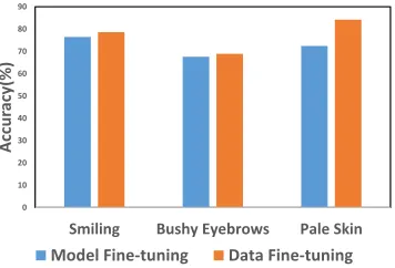
0 10 20 30 40 50 60 70 80 90
Smiling Bushy Eyebrows Pale Skin
Acc
ur
acy
(%)
Model Fine-tuning Data Fine-tuning
Figure 10: Comparing the results of Data Fine-tuning ver-sus Model Fine-tuning on the LFW dataset using a model trained on the CelebA dataset.
trained on the CelebA dataset. On comparing the results on MUCT and LFW datasets, it is observed that data fine-tuning performs better than model fine-fine-tuning for both the datasets. Experimental results obtained with other three at-tributes are shown in Figure 10, which also indicate that data fine-tuning outperforms model fine-tuning. Experiments are also performed by combining model fine-tuning with data fine-tuning. For this purpose, an iterative approach is fol-lowed, where data fine-tuning and model fine-tuning are per-formed iteratively. It is observed that the combination of model fine-tuning and data fine-tuning further enhances the results. However, such a combination is not useful for black-box systems where model fine-tuning is not possible.
Conclusion
is a challenging task. To address this situation, in this re-search a novel concept of data fine-tuning is proposed. Data fine-tuning refers to the process of adjusting the input data according to the behavior of the pre-trained model. The pro-posed data fine-tuning algorithm is designed using adver-sarial perturbation. Multiple experiments are performed to evaluate the performance of the proposed algorithm. It is observed that data fine-tuning enhances the performance of black box models. A comparison of data fine-tuning with model fine-tuning is also performed. We postulate that data tuning can be an exciting alternative to model fine-tuning, particularly for black-box systems.
Acknowledgements
Vatsa and Singh are partially supported through Infosys Center for AI at IIIT Delhi, India. The authors acknowledge Shruti Nagpal for her constructive and useful feedback.
References
Carlini, N., and Wagner, D. 2016. Defensive distillation is not
robust to adversarial examples.arXiv preprint arXiv:1607.04311.
Carlini, N., and Wagner, D. 2017. Towards evaluating the
robust-ness of neural networks. InIEEE Symposium on Security and
Pri-vacy, 39–57.
Chhabra, S.; Singh, R.; Vatsa, M.; and Gupta, G. 2018.
Anonymiz-ing k-facial attributes via adversarial perturbations. In
Interna-tional Joint Conference on Artificial Intelligence, 656–662. Ding, C., and Tao, D. 2018. Trunk-branch ensemble convolutional
neural networks for video-based face recognition. IEEE
transac-tions on Pattern Analysis and Machine Intelligence40(4):1002– 1014.
Fan, Y.; Lu, X.; Li, D.; and Liu, Y. 2016. Video-based emotion
recognition using cnn-rnn and c3d hybrid networks. In18th ACM
International Conference on Multimodal Interaction, 445–450. Goel, A.; Singh, A.; Agarwal, A.; Vatsa, M.; and Singh, R. 2018. Smartbox: Benchmarking adversarial detection and mitigation
al-gorithms for face recognition. IEEE International Conference on
Biometrics: Theory, Applications, and Systems.
Goswami, G.; Ratha, N.; Agarwal, A.; Singh, R.; and Vatsa, M. 2018. Unravelling robustness of deep learning based face
recog-nition against adversarial attacks. InAssociation for the
Advance-ment of Artificial Intelligence, 6829–6836.
Hand, E. M.; Castillo, C. D.; and Chellappa, R. 2018. Doing the best we can with what we have: Multi-label balancing with
selec-tive learning for attribute prediction. InAssociation for the
Ad-vancement of Artificial Intelligence, 6878–6885.
Huang, G. B.; Mattar, M.; Berg, T.; and Learned-Miller, E. 2008. Labeled faces in the wild: A database forstudying face
recogni-tion in unconstrained environments. InWorkshop on faces
in’Real-Life’Images: detection, alignment, and recognition.
Jain, Y. K., and Bhandare, S. K. 2011. Min max
normaliza-tion based data perturbanormaliza-tion method for privacy protecnormaliza-tion.
In-ternational Journal of Computer & Communication Technology 2(8):45–50.
Kurakin, A.; Goodfellow, I.; and Bengio, S. 2016. Adversarial
examples in the physical world.arXiv preprint arXiv:1607.02533.
Last, M.; Tassa, T.; Zhmudyak, A.; and Shmueli, E. 2014. Improv-ing accuracy of classification models induced from anonymized
datasets.Information Sciences256:138–161.
Li, X., and Zhou, Z. 2018. Secure support vector machines with
data perturbation. InChinese Control And Decision Conference,
1170–1175.
Liu, Z.; Luo, P.; Wang, X.; and Tang, X. 2015. Deep learning
face attributes in the wild. InIEEE International Conference on
Computer Vision, 3730–3738.
Milborrow, S.; Morkel, J.; and Nicolls, F. 2010. The MUCT
land-marked face database. Pattern Recognition Association of South
Africa201(0).
Moosavi-Dezfooli, S.-M.; Fawzi, A.; Fawzi, O.; and Frossard, P.
2017. Universal adversarial perturbations. InIEEE Conference on
Computer Vision and Pattern Recognition, 86–94.
Papernot, N.; McDaniel, P.; Jha, S.; Fredrikson, M.; Celik, Z. B.; and Swami, A. 2016. The limitations of deep learning in
adver-sarial settings. InIEEE European Symposium on Security and
Pri-vacy, 372–387.
Parkhi, O. M.; Vedaldi, A.; Zisserman, A.; et al. 2015. Deep
face recognition. InBritish Machine Vision Conference, volume 1,
41.1–41.12.
Salamon, J., and Bello, J. P. 2017. Deep convolutional neural networks and data augmentation for environmental sound
classifi-cation.IEEE Signal Processing Letters24(3):279–283.
Su, J.; Vargas, D. V.; and Kouichi, S. 2017. One pixel attack for
fooling deep neural networks. arXiv preprint arXiv:1710.08864.
Szegedy, C.; Zaremba, W.; Sutskever, I.; Bruna, J.; Erhan, D.; Goodfellow, I.; and Fergus, R. 2013. Intriguing properties of neural
networks.arXiv preprint arXiv:1312.6199.
Um, T. T.; Pfister, F. M.; Pichler, D.; Endo, S.; Lang, M.; Hirche, S.; Fietzek, U.; and Kuli´c, D. 2017. Data augmentation of wearable sensor data for parkinson’s disease monitoring using convolutional
neural networks. InACM International Conference on Multimodal
Interaction, 216–220.
Wu, E.; Wu, K.; Cox, D.; and Lotter, W. 2018. Conditional infilling
gans for data augmentation in mammogram classification. arXiv
preprint arXiv:1807.08093.
Xie, C.; Wang, J.; Zhang, Z.; Ren, Z.; and Yuille, A. 2017.
Mit-igating adversarial effects through randomization. arXiv preprint