The Thirty-Third AAAI Conference on Artificial Intelligence (AAAI-19)
Deep Video Frame Interpolation Using Cyclic Frame Generation
Yu-Lun Liu,
1,2,3Yi-Tung Liao,
1,2Yen-Yu Lin,
1Yung-Yu Chuang
1,21Academia Sinica,2National Taiwan University,3MediaTek
{yulunliu, queenieliaw}@cmlab.csie.ntu.edu.tw, [email protected], [email protected]
Abstract
Video frame interpolation algorithms predict intermediate frames to produce videos with higher frame rates and smooth view transitions given two consecutive frames as inputs. We propose that: synthesized frames are more reliable if they can be used to reconstruct the input frames with high qual-ity. Based on this idea, we introduce a new loss term, the
cycle consistency loss. The cycle consistency loss can bet-ter utilize the training data to not only enhance the inbet-terpo- interpo-lation results, but also maintain the performance better with less training data. It can be integrated into any frame inter-polation network and trained in an end-to-end manner. In ad-dition to the cycle consistency loss, we propose two exten-sions: motion linearity loss and edge-guided training. The motion linearity loss approximates the motion between two input frames to be linear and regularizes the training. By ap-plying edge-guided training, we further improve results by in-tegrating edge information into training. Both qualitative and quantitative experiments demonstrate that our model outper-forms the state-of-the-art methods. The source codes of the proposed method and more experimental results will be avail-able at https://github.com/alex04072000/CyclicGen.
Introduction
High-frame-rate videos with temporally coherent content are preferable, but acquiring such videos often requires higher power consumption and more storage. To compro-mise between the user experience and the acquiring cost,
video frame interpolation, e.g., (Liu et al. 2017; Niklaus, Mai, and Liu 2017b), has drawn increasing attention in the field of computer vision and video processing. It aims at upscaling video frame rates by synthesizing spatially and temporally consistent intermediate frames, and can produce high-quality videos with smooth view transition.
Convolutional neural networks (CNNs) (Krizhevsky, Sutskever, and Hinton 2012) have been employed in many modern methods for video frame interpolation (Niklaus, Mai, and Liu 2017a; 2017b; Liu et al. 2017; Long et al. 2016). These CNN-based methods often integrate motion prediction into video pixel generation, and can work with-out using hard-to-get dense flow fields as training data. Em-powered by CNNs, these methods show excellent abilities
Copyright c2019, Association for the Advancement of Artificial Intelligence (www.aaai.org). All rights reserved.
CNN
CNN
CNN
𝐼0.5′ 𝐼0
𝐼1
𝐼2
𝐼1.5′
𝐼1′′
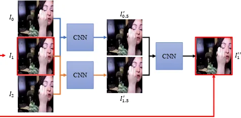
Figure 1: Given three consecutive frames,I0,I1, andI2, the proposed CNN-based model aims to produce high-quality interpolated frames, I00.5 andI10.5. To this end, the model maps the given frames to the interpolated frames and then map them back by constructingI100through interpolating be-tweenI00.5andI10.5. The proposed cycle consistency loss fa-cilitates model learning by enforcing the similarity between I1andI100.
to learn the mapping between two consecutive frames and the intermediate frame, and alleviate the problems caused by occlusions and varying lighting conditions. Despite the en-couraging progress, video frame interpolation still remains quite challenging: The interpolated frames are usually over-smoothed/blurred and have artifacts (Liang et al. 2017). This situation becomes even worse in image regions with large motions or rich textures.
This paper addresses the aforementioned issues. Our idea is built on thereverse mappingfrom the interpolated frames to the given frames. Consider a model that is derived to generate the interpolated frame by taking two consecu-tive frames as inputs. If the interpolated frames are over-smoothed or have artifacts, the reverse mapping is unlikely to be well performed by the same model. Inspired by this observation, we implement forward-backward consistency
problems of over-smoothed results and artifacts. In addition to improving performance, this loss constrains the training process, and makes the resultant model more robust even when fewer training data are available. Figure 1 illustrates the basic idea of the cycle consistency loss for video inter-polation.
Two extensions, motion linearity loss and edge guided training, are further proposed to address the difficulties of synthesizing frames in the regions with large motions and rich textures, respectively. The motion linearity loss assumes that the view transition is linear with respect to time over consecutive frames in a short period of time. The assumption effectively regularizes network training, and improves the interpolation results. Motivated by the quality degradation of the interpolated frames in highly textured areas, we aug-ment the input with edge information. The generated frames are then improved by better preserving the edge structure. The two extensions complement the cycle consistency loss, and result in considerable performance gains.
We evaluate the performance of our method on three benchmarks, including the UCF101 dataset (Soomro, Za-mir, and Shah 2012), a high-quality video, See You Again, (Niklaus, Mai, and Liu 2017b), and theMiddlebury optical flow dataset (Baker et al. 2011). The experimental results show that our method performs favorably against the state-of-the-art methods. We also conduct ablation studies to analyze the impact of the proposed cycle consistency loss, motion linearity loss, and edge guided training individually. Additionally, we demonstrate that the cycle consistency loss makes the most of training data, and results in a model ro-bust to the issue of few training data.
Related Work
This section reviews the topics relevant to this work. We first describe previous methods for video frame interpolation and contrast the proposed method with them. Next, we review the applications of the cycle constraint that the proposed cy-cle consistency loss roots from.
Video Frame Interpolation
Conventional methods (Baker et al. 2011; Werlberger et al. 2011; Yu et al. 2013) for frame interpolation usually es-timate dense motion correspondences between consecutive frames via stereo matching or optical flow prediction, and can synthesize intermediate frames based on the estimated correspondences. Inheriting from correspondence estima-tion, these methods induce computation-intensive optimiza-tion and are less efficient. Furthermore, these approaches tend to produce artifacts around object boundaries.
CNNs have been shown effective in optical flow estima-tion such as (Bailer, Taetz, and Stricker 2015; Dosovitskiy et al. 2015; Gadot and Wolf 2016; G¨uney and Geiger 2016; Teney and Hebert 2016; Tran et al. 2016; Weinzaepfel et al. 2013). These CNN-based methods for flow field predic-tion need training data in the form of dense correspondences, which are quite hard to annotate. Besides, since their goal is to generate optical flow, the interpolated frames based on optical flow often have artifacts.
Some frame synthesis methods leverage CNNs to directly generate images (Goodfellow et al. 2014) and videos (Von-drick, Pirsiavash, and Torralba 2016; Xue et al. 2016). Thus, they do not use dense correspondences as training data but the ground-truth intermediate frames. However, these methods still suffer from blurred results and artifacts. Liu et al. (Liu et al. 2017) addressed the problem of blurred results by referring to coherent regions of pixels in exist-ing frames and employexist-ing a network layer regardexist-ing optical flow. Their method makes the synthesized frames sharper, but the problem of artifacts remains unsolved. Other meth-ods (Niklaus, Mai, and Liu 2017a; 2017b) combine motion estimation and frame synthesis into a single convolution step. They estimate spatially-varying kernels for each out-put pixel, and apply them to inout-put frames for frame interpo-lation. Despite the effectiveness, these methods need pixel-specific kernel estimation, and consume high computation power and storage usage, especially for high-resolution frame synthesis.
The current state-of-the-art methods (Jiang et al. 2018; Niklaus and Liu 2018) employ CNNs to predict bi-directional optical flow between the input images, and use another CNN model to synthesize interpolated images based on the predicted flow. However, these methods either require additional training data for optical flow estimation or need substantial training time.
Unlike most existing methods that enhance frame inter-polation by designing more powerful deep features or ar-chitectures, our method mitigates the aforementioned draw-backs by utilizing the cycle consistency loss with two ex-tensions. The advantages of our method are three-fold. First, our method achieves superior performance to the state-of-the-arts by addressing the issues of blurry results and arti-facts. Second, while existing methods require more training data to learn powerful features or networks, we show that our method is more robust against the issue of insufficient training data. Third, using the cycle consistency loss does not increase the model parameters. Thus, both the training and inference costs remain almost unchanged. These nice properties distinguish our method from prior work.
Cycle Constraint
𝐹0→1
Warp
𝐹1→2
Warp
𝐹0.5→1.5 𝐼1′′
Warp
𝐼1
ℒ𝑐
𝐼0
𝐼1 𝐸1 𝐸0
𝐼1
𝐼2 𝐸2
𝐸1 𝐼0.5
′
𝐼1.5′ 𝐸1.5′ 𝐸0.5′
𝐼0
𝐼2
𝑓
𝐹0→2 𝐼1′
Warp
𝐼1
ℒ𝑟
𝐸0
𝐸2
HED
ℒ𝑚
(a) Stage 1 (b) Stage 2
: image : flow map : ground-truth : loss term : baseline model
𝑓
𝑓
𝑓
Figure 2: Approach overview. Our approach implements a two-stage optimization process. (a) At the first stage, the baseline modelf is pre-trained. (b) At the second stage, the baseline model is duplicated three times. The four models share weights and are fine-tuned by taking into account the proposed cycle consistency lossLc, motion linearity lossLm, and edge guided training. After training, the optimized modelfperforms video frame interpolation at the inference phase. See text for details.
To the best of our knowledge, this work makes the first attempt to improve video frame interpolation by leveraging cycle consistency. We design a two-stage optimization pro-cedure so that the interpolation model shared by both map-ping directions in the cycle constraint can be learned stably. It turns out that our method can greatly improve the quality of interpolation without incurring extra learnable parame-ters. In addition, the concept of cycle consistency is extended by taking application-specific knowledge into account, and can address the degraded performance in regions with large motions or rich textures.
Proposed Approach
Given a set of training data D = {In,0, In,1, In,2}Nn=1, each of which is a triplet containing three consecutive video frames, we aim to learn a deep model that takes two con-secutive frames as inputs and can predict their interme-diate frame of high quality. Applying the learned model to all consecutive frames of a video doubles its frame rate. Repeatedly applying the model k times upscales the frame rate by a factor of 2k. For example, given the in-put framesS = {I0, I1, I2, ..., IN}, our model first gener-ates framesS0 ={I0.5, I1.5, I2.5, ..., IN−0.5}for2× inter-polation. Then, it is applied again toS∪S0 and produces S00={I0.25, I0.75, ..., IN−0.25}for4×interpolation.
Our method implements a two-stage training process. Its network architecture is shown in Figure 2. Our method is featured with three newly proposed components, i.e., the cy-cle consistency loss, motion linearity loss, and edge guided training. The cycle consistency loss boosts the model to pro-duce plausible intermediate frames so that these frames can be used to reversely reconstruct the given frames. The mo-tion linearity loss regularizes the estimamo-tion of momo-tions in training. Edge guided training helps preserve the edge struc-ture. We will describe the three components below.
Cycle Consistency Loss
L
cConventional loss functions, such as the `1-norm loss, are not fully consistent with human perception when assess-ing the quality of interpolated frames. Minimizassess-ing the ` 1-norm loss often leads to over-smoothed frames or artifacts, as shown in Figures 3(a) and 3(b), since these unfavorable effects only yield subtle increase in the loss. Motivated by the observation that the over-smoothed interpolated frames with artifacts cannot well reconstruct the original frames via the same interpolation model, we propose the cycle consis-tency loss Lc, which ensures the quality of reverse frame generation, i.e., generating the original frames with the in-terpolated frames as input. In this way, these unfavorable effects can be alleviated implicitly by using the cycle con-sistency loss, as shown in Figure 3(c).
Consider a baseline interpolation model that takes two consecutive frames as inputs and synthesizes the interme-diate frame between them. The baseline model can be ap-plied to each tripletn,(In,0, In,1, In,2), in the training setD, whereIn,0andIn,2 serve as the input whileIn,1is the de-sired output. Since each triplet acts as the input to the model, we sometimes omit the indexnfor brevity in the paper. Sev-eral existing methods, such asAdaConv(Niklaus, Mai, and Liu 2017a) andSepConv(Niklaus, Mai, and Liu 2017b), can serve as the baseline model. In this work, we choosedeep voxel flow (DVF) (Liu et al. 2017) as the baseline for its simplicity and good performance. The DVF model learns to synthesize the in-between frame from the input frames by warping the input frames with the predicted flow map and mask. Refer to the original paper of DVF (Liu et al. 2017) for its details.
𝐼0
(a)
𝐼1
𝐼2
(b) (c)
𝐼0.5′
𝐼1′′
𝐼0.5′
𝐼1.5′ 𝐼1.5′
𝐼1′′
Figure 3: (a) Three input frames,I0,I1, andI2, for inter-polation. (b) Two interpolated frames,I00.5 andI10.5, by us-ing the`1-norm loss. The reconstructedI1, i.e.,I100, is ob-tained by applying the same interpolation model toI00.5and I10.5. As can be observed, the issues of artifacts (the region in the yellow box) and over-smoothed results (the region in the blue box) are present in both the interpolated frames and the reconstructed frame. (c) The same figures as those in (b) except the cycle consistence loss is integrated into the loss function for learning the interpolation model. The issues of artifacts and over-smoothed results are greatly alleviated.
each training triplet by using the`1-norm lossLrwherer stands forreconstruction, i.e.,
Lr= N
X
n=1
||f(In,0, In,2)−In,1||1= N
X
n=1
||In,0 1−In,1||1,
(1) wheref is the baseline model.
At the second stage, we duplicate the pre-trained model f three times as shown in Figure 2 for introducing the cycle consistency loss. For a triplet(I0, I1, I2), the first two dupli-cated models respectively take(I0, I1)and(I1, I2)as input, and generate intermediate frames,I00.5andI10.5, which then serve as the input to the third duplicated model to produce the reconstructed I1, i.e., I100. The cycle consistency loss minimizes the difference between the input framesI1and its reconstructed versionI100. Specifically, the learnable parame-ters of the baseline modelfand its three duplicated counter-parts areshared. At the second stage, the four shared-weight models are trained in an end-to-end manner with the follow-ing objective function:
L=Lr+Lc= N
X
n=1
||In,0 1−In,1||1+||In,001−In,1||1, (2)
whereIn,001 = f(In,0 0.5, In,0 1.5),In,0 0.5 = f(In,0, In,1)and
0 0.01 0.02 0.03 0.04 0.05
1 2 3 4 5 6 7 8 9 10
Me
an squa
re
d e
rr
or
(MS
E)
Gradient bins (low →high)
(a) (b)
0 1 2 3 4
1 2 3 4 5 6 7 8 9 10
Number
of pix
els
(10
6)
Gradient bins (low →high)
Figure 4: Interpolation errors of pixels on the DVF testing set. Pixels are divided into ten bins according to their gra-dient magnitudes. (a) Histogram of gragra-dient magnitudes. (b) Average interpolation error for pixels in each bin. The larger the gradient, the higher the interpolation error.
I0
n,1.5 =f(In,1, In,2)are the generated frames by the three shared-weight models, respectively.
Motion Linearity Loss
L
mRegions with large motions cause dramatic appearance change. Thereby, interpolation on such regions is quite dif-ficult. To address this issue, we assume the time interval be-tween two consecutive frames is short enough so that the motion is linear between the two frames. This assumption helps reduce the uncertainty of motion and alleviate approx-imation errors in most cases.
Based on the assumption, the motion linearity lossLmis developed to regularize the optical flow estimation in a self-supervised fashion. In the two-stage training process, the time intervals between consecutive frames at the first stage are twice as long as those at the second stage. With the mo-tion linearity assumpmo-tion, the model pre-trained at the first stage generates flow fields with magnitudes twice as large as the duplicated models at the second stage.
In Figure 2, blue blocks represent the estimated flow maps upon which the motion linearity lossLmis applied. Specif-ically, this loss is defined by
Lm= N
X
n=1
kFn,0→2−2·Fn,0.5→1.5k22, (3)
whereF denotes the flow map and its subscript indicates its data index and the time interval of its input frames.
Edge-guided Training
E
To compute the edge map of an image, we tried sev-eral algorithms, including (Canny 1986; Kanopoulos, Vas-anthavada, and Baker 1988; Marr and Hildreth 1980; Xie and Tu 2015). We ended up with using the CNN-based model, holistically-nested edge detection (HED) (Xie and Tu 2015), for its performance. In addition, by using CNN-based HED, our method remains end-to-end trainable. As shown in Figure 2, we obtain the edge maps for the two in-put frames to the modelf via HED, and augment them as part of the input to the model.
Implementation Details
Our method is built on the top of DVF (deep voxel flow) model (Liu et al. 2017) and shares the same setting with it. DVF employs a CNN model to estimate the motion between two consecutive frames and copies pixels from the two frames accordingly to reconstruct the intermediate frame. The optimization is performed with two stages, whose ob-jective functions are respectively specified below
Ls1 =LrandLs2=Lr+λcLc+λmLm, (4)
whereLr,Lc, andLmare defined in Eq. (1), Eq. (2), and Eq. (3), respectively. The weightsλcandλmare determined empirically using a validation set.λc= 1andλm= 0.1are used in all experiments. Every component of our network is differentiable. Thus, our model is end-to-end trainable. The optimization is performed by Adam optimizer (Kingma and Ba 2015). The batch size is set to8, while the learning rate is fixed to0.0001during the first stage and reduced to0.00001
during the second stage optimization.
We had tried to train the model in an end-to-end manner without the first stage. The performance of the network is less reliable due to the lack of the better initialization ob-tained in the first stage. The result reveals that the initializa-tion from the first stage is beneficial in our case. We had also tried the cycle consistency with a loop of three steps. How-ever, it only resulted in a subtle improvement but made the network much more complex during training. Thus, we only use the two-step cycle in this work.
Experiments
In this section, we report the datasets used in the experi-ments, ablation studies and comparisons with the state of the arts. We also discuss the limitations of the proposed method.
Datasets
We train our model using the training set of the UCF101 dataset (Soomro, Zamir, and Shah 2012). A training video is split into many triplets, each containing three consecu-tive frames. For each triplet, the middle frame serves as the ground truth while the other two are inputs. To have more challenging samples for training, we select the triplets with more obvious motion by choosing those with lower PSNR values between input frames. Approximately 280,000 triplets are selected to form the training set. For reducing memory consumption, all frames are scaled to the resolution of256×256.
PSNR SSIM
Baseline (DVF) 35.89 0.945
+ Cycle 36.71 (+0.82) 0.950 (+0.005)
+ Cycle + Motion 36.85 (+0.96) 0.950 (+0.005)
+ Cycle + Edge 36.86 (+0.97) 0.952 (+0.007) full model 36.96(+1.07) 0.953(+0.008)
Table 1: Ablation studies. The numbers in parenthesis indi-cate improvement against the baseline. (Cycle: cycle consis-tency loss;Motion: motion linearity loss;Edge: edge-guided training. )
Training size Baseline (DVF) Ours (Lc+Lm)
1 35.98 36.85
1/10 35.71 (-0.27) 36.83 (-0.02) 1/100 35.43 (-0.55) 36.70 (-0.15) 1/1000 34.42 (-1.56) 36.10 (-0.75)
Table 2: Evaluation of models with different training data sizes. The average PSNR (dB) for the UCF101 testing set is reported. The numbers in parenthesis indicate performance drop compared with the same model trained with full data.
We test the proposed network on several datasets, in-cluding UCF101 (Soomro, Zamir, and Shah 2012), Middle-bury flow benchmark (Baker et al. 2011), and a high-quality YouTube video:See You Againby Wiz Khalifa. For UCF101 andSee You Again, in every triple, the first and third frames are used as inputs to predict the second one. The UCF101 testing set consists of 379 sequences provided by (Liu et al. 2017). For the Middlebury flow benchmark, we submit our interpolation results of the eight test sequences to the eval-uation website. For quantitative evaleval-uation, we report both Peak Signal-to-Noise Ratio (PSNR) and Structural Similar-ity Index (SSIM) between the synthesized and real frames.
Ablation Studies
For understanding the performance of the proposed compo-nents, we conduct ablation studies on the UCF101 testing set provided by DVF. As our model is based on DVF, we consider it as the baseline and compare its results with the ones of applying the proposed components, including the cy-cle consistency loss, motion linearity loss, and edge-guided training, to investigate effectiveness of each component.
Inputs Ground truth(a) Baseline(b) (DVF)
(c)
+ Cycle + Cycle (d) + Motion
(e) + Cycle
+ Edge
(e) Full model
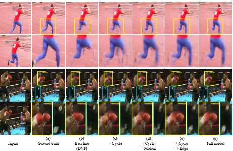
Figure 5: Visual comparisons for the ablation studies.
Inputs
(a) Ground truth
(b) Baseline
(DVF)
(c) + Cycle
(d) + Cycle + Motion
Figure 6: Visual comparisons for the motion linearity loss.
Motion Linearity LossLm Table 1 reports that the mo-tion linearity loss brings an addimo-tional 0.14dB gain on the top of cyclic generation. It is because the assumption of lin-ear motion helps restrict frame synthesis within the subspace with more plausible motion. Figure 5 and Figure 6 give vi-sual examples. As an example, the hand in Figure 6(d) looks sharper with the help of the motion linearity assumption.
Edge-Guided Training E As shown in Table 1, edge-guided training gains 0.15dB to further improve the perfor-mance of cyclic generation. It is because the information provided by edge maps helps guide interpolation and im-prove performance in the areas with strong gradients.
Fig-Inputs
(a) Ground truth
(b) Baseline
(DVF)
(c) + Cycle
(d) + Cycle
+ Edge
Figure 7: Visual comparisons for the edge-guided training.
ure 5 and Figure 7 show examples where edge-guided train-ing helps. For example, the dashed arc in the free throw lane becomes visible in Figure 7(d) with the help of edge-guided training.
Impact of the Number of Training Samples Our cyclic frame generation method uses the generated frames as train-ing data for the second-stage traintrain-ing. It has the potential to utilize the data more effectively. We conduct experiments to verify the point by varying the amount of training data. The full UCF101 training data contain approximately 280,000 triplets. We reduce the training data to 1/10, 1/100 and
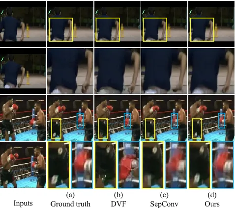
Inputs Ground truth(a) (b) DVF
(c) SepConv
(d) Ours
Figure 8: Visual comparisons for examples from UCF101.
UCF101 See You Again
PSNR SSIM PSNR SSIM
DVF 35.89 0.945 40.15 0.958
SepConv 36.49 0.950 41.01 0.968
Ours 36.96 0.953 41.67 0.968
Table 3: Quantitative comparisons on the UCF101 testing set and the high-quality videoSee You Again.
and our method (Lc+Lm) with different amounts of training data. It is clear that the proposed method maintains perfor-mance better with less training data. For example, when us-ing1/10of the training data, our method almost performs as well as the one using full data by only dropping 0.02dB. For the same amount of data, the baseline method has already dropped 0.27dB. When using only 1/1000of the training data (meaning merely 280 triplets for training), our method can still keep very good performance (36.10dB), even better than the baseline method trained with full data (35.98dB). The experiment shows that our method utilizes the training data very well. It suffers less from over-fitting and is robust even with little training data.
Comparisons with State-of-the-Art Methods
We compare our method mainly with two state-of-the-art methods, separable adaptive convolution (Sep-Conv) (Niklaus, Mai, and Liu 2017b) and deep voxel flow (DVF) (Liu et al. 2017), with publicly available executa-bles. While evaluating on the Middlebury flow benchmark, we also compare with the top performance methods listed in the benchmark website. The supplementary video shows interpolation results of our method for a8×frame rate.
UCF101 For UCF101, we compute both PSNR and SSIM using the motion masks provided by (Liu et al. 2017). As re-ported in Table 3, for UCF101, our method outperforms both
DVF and SepConv, by 1.07dB and 0.47dB in PSNR respec-tively. Figure 8 shows visual comparisons of these methods.
See You Again For testing generalization of the model, we apply the model trained on UCF101 to a high-quality YouTube video,See You Again. It has 5,683 frames with the resolution960×540. We take odd-number frames as inputs and synthesize the even-number frames. The right part of Ta-ble 3 reports PSNR and SSIM values of compared methods onSee You Again. Our method outperforms the others.
Middlebury To better accommodate the large appear-ance difference between UCF101 and Middlebury, we fine-tune our model using the training set provided by Mid-dlebury, which contains only 168 frames. Table 4 reports the interpolation errors (IE) of our model and five top-performance methods in Middlebury’s list on the eight test-ing sequences of the benchmark. The compared methods include (1) synthesis-based methods which directly gener-ate interpolgener-ated frames: CtxSyn (Niklaus and Liu 2018), SepConv (Niklaus, Mai, and Liu 2017b), and SuperSlomo (Jiang et al. 2018); and flow-based methods which utilize op-tical flows for frame interpolation: MDP-Flow2 (Xu, Jia, and Matsushita 2012) and DeepFlow (Weinzaepfel et al. 2013). At the time when the paper is submitted, CtxSyn ranks the first and all five compared methods are among top six. Our model achieves the best average performance and owns the best records for 5 out of all 8 sequences. Note that the last four sequences contain real images. It indicates that our method performs particularly well on real-scene sequences. Fine-tuning with 168 frames also shows that our approach performs well with little training data. Figure 9 shows visual comparisons on examples from the Middlebury benchmark.
Limitations
Although our method provides good improvement, it has some limitations. First, dealing with the areas with large mo-tions remains challenging to our method. As shown in Fig-ures 5 and 9, although the cycle consistency and motion lin-earity losses jointly alleviate the interpolation errors, there are still interpolation errors in the regions with large tions. Second, the motion linearity loss assumes linear mo-tion, but the linearity assumption may not hold in videos at very low frame rates, which likely would cause interpolation errors. In addition, our method performs repeated interpola-tion. Hence, it only upscales the frame rate by a factor of
2N, instead of an arbitrary frame rate that a user desires.
Conclusion
AVERAGE Mequon Schefflera Urban Teddy Backyard Basketball Dumptruck Evergreen
all disc. unt. all disc. unt. all disc. unt. all disc. unt. all disc. unt. all disc. unt. all disc. unt. all disc. unt. all disc. unt.
Ours 4.20 6.16 1.97 2.26 3.32 1.42 3.19 4.01 2.21 2.76 4.05 1.62 4.97 5.92 3.79 8.00 9.84 3.13 3.36 5.65 2.17 4.55 9.68 1.42 4.48 6.84 1.52
CtxSyn 5.28 8.00 2.19 2.24 3.72 1.04 2.96 4.16 1.35 4.32 3.42 3.18 4.21 5.46 3.00 9.59 11.9 3.46 5.22 9.76 2.22 7.02 15.4 1.58 6.66 10.2 1.69
SuperSlomo 5.31 8.39 2.12 2.51 4.32 1.25 3.66 5.06 1.93 2.91 4.00 1.41 5.05 6.27 3.66 9.56 11.9 3.30 5.37 10.2 2.24 6.69 15.0 1.53 6.73 10.4 1.66
SepConv 5.61 8.74 2.33 2.52 4.83 1.11 3.56 5.04 1.90 4.17 4.15 2.86 5.41 6.81 3.88 10.2 12.8 3.37 5.47 10.4 2.21 6.88 15.6 1.72 6.63 10.3 1.62
MDP-Flow2 5.83 9.69 2.15 2.89 5.38 1.19 3.47 5.07 1.26 3.66 6.10 2.48 5.20 7.48 3.14 10.2 12.8 3.61 6.13 11.8 2.31 7.36 16.8 1.49 7.75 12.1 1.69
DeepFlow 5.97 9.79 2.05 2.98 5.67 1.22 3.88 5.78 1.52 3.62 5.93 1.34 5.39 7.20 3.17 11.0 13.9 3.63 5.91 11.3 2.29 7.14 16.3 1.49 7.80 12.2 1.70
Table 4: Quantitative comparisons on the Middlebury benchmark. The table reports the interpolation errors.disc.: regions with discontinuous motion.unt.: textureless regions.
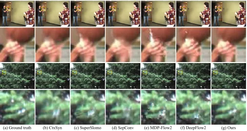
(a) Ground truth (b) CtxSyn (c) SuperSlomo (d) SepConv (e) MDP-Flow2 (f) DeepFlow2 (g) Ours
Figure 9: Visual comparisons of our method and five competing methods on examples from the Middlebury benchmark.
approach better utilizes the training data, not only enhanc-ing the interpolation results, but also reachenhanc-ing better perfor-mance with less training data.
Acknowledgments
This work was supported in part by Ministry of Science and Technology (MOST) under grants MOST 107-2628-E-001-005-MY3, MOST107-2221-E-002-147-MY3, and MOST Joint Research Center for AI Technology and All Vista Healthcare under grant 107-2634-F-002-007.
References
Bailer, C.; Taetz, B.; and Stricker, D. 2015. Flow fields: Dense correspondence fields for highly accurate large dis-placement optical flow estimation. InProceedings of IEEE ICCV.
Baker, S.; Scharstein, D.; Lewis, J.; Roth, S.; Black, M. J.; and Szeliski, R. 2011. A database and evaluation method-ology for optical flow. International Journal of Computer Vision92(1):1–31.
Brislin, R. W. 1970. Back-translation for cross-cultural re-search. Journal of cross-cultural psychology1(3):185–216. Canny, J. 1986. A computational approach to edge detec-tion. IEEE Transactions on Pattern Analysis and Machine Intelligence8(6):679–698.
Dosovitskiy, A.; Fischer, P.; Ilg, E.; Hausser, P.; Hazirbas, C.; Golkov, V.; van der Smagt, P.; Cremers, D.; and Brox, T. 2015. FlowNet: Learning optical flow with convolutional networks. InProceedings of IEEE ICCV.
Gadot, D., and Wolf, L. 2016. PatchBatch: a batch aug-mented loss for optical flow. InProceedings of IEEE CVPR. Godard, C.; Mac Aodha, O.; and Brostow, G. J. 2017. Un-supervised monocular depth estimation with left-right con-sistency. InProceedings of IEEE CVPR.
Goodfellow, I.; Pouget-Abadie, J.; Mirza, M.; Xu, B.; Warde-Farley, D.; Ozair, S.; Courville, A.; and Bengio, Y. 2014. Generative adversarial nets. InProceedings of NIPS. G¨uney, F., and Geiger, A. 2016. Deep discrete flow. In
Proceedings of ACCV.
Eleventh Eurographics/ACMSIGGRAPH Symposium on Ge-ometry Processing.
Jiang, H.; Sun, D.; Jampani, V.; Yang, M.-H.; Learned-Miller, E.; and Kautz, J. 2018. Super slomo: High quality estimation of multiple intermediate frames for video inter-polation. InProceedings of IEEE CVPR.
Kanopoulos, N.; Vasanthavada, N.; and Baker, R. L. 1988. Design of an image edge detection filter using the Sobel op-erator.IEEE Journal of Solid-State Circuits23(2):358–367. Kingma, D. P., and Ba, J. 2015. Adam: A method for stochastic optimization. InProceedings of ICLR.
Krizhevsky, A.; Sutskever, I.; and Hinton, G. E. 2012. Im-ageNet classification with deep convolutional neural net-works. InProceedings of NIPS.
Liang, X.; Lee, L.; Dai, W.; and Xing, E. P. 2017. Dual motion GAN for future-flow embedded video prediction. In
Proceedings of IEEE ICCV.
Liu, Z.; Yeh, R.; Tang, X.; Liu, Y.; and Agarwala, A. 2017. Video frame synthesis using deep voxel flow. InProceedings of IEEE ICCV.
Long, G.; Kneip, L.; Alvarez, J. M.; Li, H.; Zhang, X.; and Yu, Q. 2016. Learning image matching by simply watching video. InProceedings of ECCV.
Marr, D., and Hildreth, E. 1980. Theory of edge detection.
Proc. R. Soc. Lond. B207:187–217.
Niklaus, S., and Liu, F. 2018. Context-aware synthesis for video frame interpolation. InProceedings of IEEE CVPR. Niklaus, S.; Mai, L.; and Liu, F. 2017a. Video frame inter-polation via adaptive convolution. InProceedings of IEEE CVPR.
Niklaus, S.; Mai, L.; and Liu, F. 2017b. Video frame inter-polation via adaptive separable convolution. InProceedings of IEEE ICCV.
Soomro, K.; Zamir, A. R.; and Shah, M. 2012. UCF101: A dataset of 101 human actions classes from videos in the wild. Technical Report CRCV-TR-12-01, University of Cen-tral Florida.
Sundaram, N.; Brox, T.; and Keutzer, K. 2010. Dense point trajectories by GPU-accelerated large displacement optical flow. InProceedings of ECCV.
Teney, D., and Hebert, M. 2016. Learning to extract motion from videos in convolutional neural networks. In Proceed-ings of ACCV.
Tran, D.; Bourdev, L.; Fergus, R.; Torresani, L.; and Paluri, M. 2016. Deep end2end voxel2voxel prediction. In Pro-ceedings of IEEE CVPR Workshops.
Vondrick, C.; Pirsiavash, H.; and Torralba, A. 2016. Gener-ating videos with scene dynamics. InProceedings of NIPS. Wang, F.; Huang, Q.; and Guibas, L. J. 2013. Image co-segmentation via consistent functional maps. InProceedings of IEEE ICCV.
Weinzaepfel, P.; Revaud, J.; Harchaoui, Z.; and Schmid, C. 2013. DeepFlow: Large displacement optical flow with deep matching. InProceedings of IEEE ICCV.
Werlberger, M.; Pock, T.; Unger, M.; and Bischof, H. 2011. Optical flow guided TV-L1 video interpolation and restora-tion. InProceedings of IEEE CVPR Workshops.
Xie, S., and Tu, Z. 2015. Holistically-nested edge detection. InProceedings of IEEE ICCV.
Xu, L.; Jia, J.; and Matsushita, Y. 2012. Motion detail pre-serving optical flow estimation. IEEE Transactions on Pat-tern Analysis and Machine Intelligence34(9):1744–1757. Xue, T.; Wu, J.; Bouman, K.; and Freeman, B. 2016. Vi-sual dynamics: Probabilistic future frame synthesis via cross convolutional networks. InProceedings of NIPS.
Yu, Z.; Li, H.; Wang, Z.; Hu, Z.; and Chen, C. W. 2013. Multi-level video frame interpolation: Exploiting the inter-action among different levels. IEEE Transactions on Cir-cuits and Systems for Video Technology23(7):1235–1248. Zach, C.; Klopschitz, M.; and Pollefeys, M. 2010. Dis-ambiguating visual relations using loop constraints. In Pro-ceedings of IEEE CVPR.
Zhou, T.; Jae Lee, Y.; Yu, S. X.; and Efros, A. A. 2015. FlowWeb: Joint image set alignment by weaving consistent, pixel-wise correspondences. InProceedings of IEEE CVPR. Zhou, T.; Krahenbuhl, P.; Aubry, M.; Huang, Q.; and Efros, A. A. 2016. Learning dense correspondence via 3D-guided cycle consistency. InProceedings of IEEE CVPR.