The Thirty-Third AAAI Conference on Artificial Intelligence (AAAI-19)
Explicitly Imposing Constraints in Deep Networks via
Conditional Gradients Gives Improved Generalization and Faster Convergence
Sathya N. Ravi, Tuan Dinh, Vishnu Suresh Lokhande, Vikas Singh
{[email protected]},{tuandinh, lokhande, vsingh}@cs.wisc.eduAbstract
A number of results have recently demonstrated the benefits of incorporating various constraints when training deep ar-chitectures in vision and machine learning. The advantages range from guarantees for statistical generalization to bet-ter accuracy to compression. But support for general con-straints within widely used libraries remains scarce and their broader deployment within many applications that can benefit from them remains under-explored. Part of the reason is that Stochastic gradient descent (SGD), the workhorse for training deep neural networks,does not natively deal with constraints with global scope very well.In this paper, we revisit a clas-sical first order scheme from numerical optimization, Condi-tional Gradients (CG), that has, thus far had limited applica-bility in training deep models. We show via rigorous analysis how various constraints can be naturally handled by modifi-cations of this algorithm. We provide convergence guarantees and show a suite ofimmediate benefitsthat are possible — from training ResNets with fewer layers but better accuracy simply by substituting in our version of CG to faster train-ing of GANs with 50% fewer epochs in image inpainttrain-ing ap-plications to provably better generalization guarantees using efficiently implementable forms of recently proposed regular-izers.
Introduction
The learning or fitting problem in deep neural networks in the supervised setting is often expressed as the following stochastic optimization problem,
min
W (x,yE)∼D
L(W; (x, y)) (1)
whereW =W1× · · · ×Wldenotes the Cartesian product of the weight matrices of the network withllayers that we seek to learn from the data(x, y)sampled from the underly-ing distributionD. Here,xcan be thought of the “features” (or predictor variables) of the data andydenotes the “labels” (or the response variable). The variableWparameterizes the function that predicts the labels given the features whose ac-curacy is measured using the loss functionL. For simplic-ity, the specification above is intentionally agnostic of the activation function we use between the layers and the spe-cific network architecture. Most common instantiations of
Copyright c2019, Association for the Advancement of Artificial Intelligence (www.aaai.org). All rights reserved.
the above task are non-convex but results in the last 5 years show that good minimizers can be found via SGD and its variants. Recent results have also explored the interplay be-tween the overparameterization of the network, its degrees of freedom and issues related to global optimality (Soudry and Carmon 2016).
Regularizers.Independent of the architecture we choose to deploy for a given task, one may often want to impose additional constraints or regularizers, pertinent to the ap-plication domain of interest. In fact, the use of task spe-cific constraints to improve the behavioral performance of
neural networks, both from a computational and statisti-cal perspective, has a long history dating back at least to the 1980s (Platt and Barr 1988; Zhang and Constantinides 1992). These ideas are being revisited (Rudd, Di Muro, and Ferrari 2014) motivated by generalization, convergence or simply as a strategy for compression (Cheng and others 2017). However, using constraints on the types of archi-tectures that are common in modern AI problems is still being actively researched by various groups. For example, (Mikolov and others 2014) demonstrated that training Re-current Networks can be accelerated by constraining a part of the recurrent matrix to be close to identity. Sparsity and low-rank encouraging constraints have shown promise in a number of settings (Tai and others 2015). In an interesting paper, (Pathak, Krahenbuhl, and Darrell 2015) showed that linear constraints on the output layer improves the accuracy on a semantic image segmentation task. (M´arquez-Neila, Salzmann, and Fua 2017) showed that hard constraints on the output layer yield competitive results on the pose estima-tion task and (Oktay and others 2017) used anatomical con-straints for cardiac image analysis. This suggests that while there are some results demonstrating the value of specific
constraints forspecificproblems, the development is still in a nascent stage. It is, therefore, not surprising that the exist-ing software libraries for deep learnexist-ing (DL) offer little to no support for hard constraints. For example, Keras only offers support for simple bound constraints.
param-eters using a few training examples. It mitigates the cost of running back propagation over the full dataset and comes with various guarantees as well (Hardt, Recht, and Singer 2016). The reader will notice that part of the reason that constraints have not been intensively explored may have to do with the interplay between constraints and the SGD al-gorithm (M´arquez-Neila, Salzmann, and Fua 2017). While some regularizers and “local” constraints are easily handled within SGD, some others require a great deal of care and can adversely affect convergence and practical runtime (Bengio 2012). There are also a broad range of constraints where SGD isunlikely to work well based on theoretical results known today— and it remains an open question in optimiza-tion (Johnson and Zhang 2013). We note that algorithms other than the standard SGD have remained a constant focus of research in the community since they offer many theo-retical advantages that can also be easily translated to prac-tice (Dauphin, de Vries, and Bengio 2015). These include adaptive sub-gradient methods such as Adagrad, the RM-Sprop algorithm, and various adaptive schemes for choosing learning rate including momentum based methods (Good-fellow, Bengio, and Courville 2016). However, notice that these methods only impose constraints in a “local” fashion since the computational cost of imposing global constraints using SGD-based methods becomes extremely high (Pathak, Krahenbuhl, and Darrell 2015).
Do we need to impose constraints?
The question of why constraints are needed for statistical learning models in vision and machine learning can be re-stated in terms of the need for regularization while learning models. Recall that regularization schemes in one form or another go nearly as far back as the study of fitting mod-els to observations of data (Wahba 1990). Broadly speaking, such schemes can be divided into two related categories: al-gebraic and statistical. Thefirstcategory may refer to prob-lems that are otherwise not possible or difficult to solve, also known as ill-posed problems (Tikhonov, Goncharsky, and Bloch 1987). For example, without introducing some addi-tional piece of information, it is not possible to solve a linear system of equationsAx=bin which the number of obser-vations (rows ofA) is less than the number of degrees of freedom (columns ofA). In thesecondcategory, one may use regularization as a way of “explaining” data using sim-ple hypotheses rather than comsim-plex ones, for examsim-ple, the minimum description length principle (Rissanen 1985). The rationale is that, complex hypotheses are less likely to be ac-curate on the unobserved samples since we need more data to train complex models. Recent developments on the theo-retical side of DL showed that imposing simple butglobalconstraints on the parameter space is an effective way of analyzing the sample complexity and generalization error (Neyshabur, Tomioka, and Srebro 2015). Hence we seek to solve,
min
W (x,yE)∼D
L(W; (x, y)) +µR(W) (2)
whereR(·)is a suitable regularization function for a fixed
µ >0. We usually assume thatR(·)is simple, in the sense
that the gradient can be computed efficiently. Using the La-grangian interpretation, Problem (2) is the same as the fol-lowing constrained formulation,
min
W (x,yE)∼D
L(W; (x, y))s.t.R(W)≤λ (3)
whereλ > 0. Note that when the loss functionL is con-vex, both the above problems are equivalent in the sense that givenµ >0in (2), there exists aλ >0in (3) such that the
optimal solutions to both the problems coincide(see Sec 1.2 in (Bach and others 2012)). In practice, both λandµ are chosen by standard procedures such as cross validation.
Finding Pareto Optimal Solutions:On the other hand, when the loss function is nonconvex as is typically the case in DL, formulation (3) is more powerful than (2). Let us see why.
For a fixedλ >0, there might be solutionsWλ∗of (3) for which there existsnoµ > 0such thatWλ∗ = Wµ∗whereas any solution of problem (2) can be obtained for someµin (3) (Section 4.7 in (Boyd and Vandenberghe 2004)). It turns out that it is easier to understand this phenomenon through Mul-tiobjective Optimization (MO). In MO, care has to be taken to even define the notion of optimality of feasible points (let alone computing them efficiently). Among various notions of optimality, we will now argue that Pareto optimality is the most suited for our goal.
Recall that our goal is to findW’s that achieve low train-ing error and are at the same time “simple” (as measured by
R). In this context, a Pareto optimal solution is a pointW
such that none ofL(W)orR(W)in (3) or (2) can be made better without making the other worse, thus capturing the essence of overfitting effectively. In practice, there are many algorithms to find Pareto optimal solutions and this is where problem (3) dominates (2). Specifically, formulation (2) falls under the category of “scalarization” technique whereas (3) is -constrained technique. It is well known that when the problem is nonconvex,-constrained technique yields pareto optimal solutions whereas scalarization technique does not (Boyd and Vandenberghe 2004)!
Finally, we should note that even when the problems (2) and (3) are equivalent, in practice, algorithms that are used to solve them can be very different.
First Order Methods: Two Representatives
To setup the stage for our development we first discuss the two broad strategies that are used to solve problems of the form shown in (3). First, a natural extension of gradient descent (GD) also known as Projected GD (PGD) may be used. Intuitively, we take a gradient step and then compute the point that is closest to the feasible set defined by the reg-ularization function. Hence, at each iteration PGD requires the solution of the following optimization problem or the so-called Projection operator,WtP GD+1 ←arg min W:R(W)≤λ
1
2kW−(Wt−ηgt)k
2 F (4)
wherekWkFis the Frobenius norm ofW,gtis (an estimate of) the gradient ofLatWtandη is the step size. In prac-tice, we computegtby using only a few training samples (or minibatch) and running backpropagation. Note that the objectiveE(x,y)∼DL(W)is smooth inW for any
probabil-ity distributionDwith a density function and is commonly referred to asstochastic smoothing. Hence, for our descrip-tions, we will assume that the derivative is well defined. Fur-thermore, when there are no constraints, (4) is simply the standard SGD method that requires optimizing a quadratic function on the feasible set. So, the main bottleneck in ex-plicitly imposing constraints with PGD is the complexity of solving (4). Even though manyR(·)do admit an efficient procedure in theory, using them for applications in training deep models has been a challenge since they may be com-plicated or not easily amenable to a GPU implementation (Taylor and others 2016; Frerix and others 2017).
So, a natural question to ask is whether there are meth-ods that are faster in the following sense: can we solve sim-pler problems at each iteration and also explicitly impose the constraints effectively? An assertive answer is provided by a scheme that falls under the second general category of first order methods: the Conditional Gradient (CG) al-gorithm (Reddi and others 2016). Recall that CG methods solve the followinglinear minimization problem at each it-erationinstead of a quadratic one
st∈arg min W g
T
tW s.t.R(W)≤λ (5)
and updateWCG
t+1 ← ηWt+ (1−η)st. While both PGD and CG guarantee convergence with mild conditions onη, it may be the case (as we will see shortly) that problems of the form (5) can bemuch simplerthan the form in (4) and hence highly suitable for training deep learning models. An additional bonus is that CG algorithms also offer nice space complexity guarantees that are also attainable in practice, making it a very promising choice for explicitlyconstrained
training of deep models.
Remark 1. Note that in order for CG algorithm (5) to be well defined, we need the feasible set to be bounded whereas this is not required for PGD (4).
To that end, we will see how the CG algorithm behaves for the regularization constraints that are commonly used.
Remark 2. Note that although the loss functionEL(W)is
nonconvex, the constraints that we need for almost all appli-cations are convex, hence, all our algorithms are guaranteed
to converge by design (Lacoste-Julien 2016; Reddi and oth-ers 2016) to a stationary point.
Categorizing “Generic” Constraints for CG
We now describe how a broad basket of “generic” con-straints broadly used in literature, can be arranged into a hi-erarchy — ranging from cases where a CG scheme is perfect and expected to yield wide-ranging improvements to situa-tions where the performance is only satisfactory and addi-tional technical development is warranted. For example, the`1-norm is often used to induce sparsity. The nuclear norm (sum of singular values) is used to induce a low rank regu-larization, often for compression and/or speed-up reasons.
So, how do we know which constraints when imposed using CG are likely to work well?In order to analyze the qualitative nature of constraints suitable for CG algorithm, we categorize the constraints into three categories based on how the updates will, computationally, and learning-wise, compare to a SGD update.
Category 1 constraints are excellent
We categorize constraints as Category 1 if both the SGD and CG updates take a similar form algebraically. The reason we call this category “excellent” is because it is easy to trans-fer the empirical knowledge that we obtained in the uncon-strained setting, specifically, learning and dropout rates to the regime where we want to explicitly impose these addi-tional constraints. Here, we see that we get quantifiable im-provements in terms of both computation and learning.
Two types of generic constraints fall into this category:1)
the Frobenius norm and2)the Nuclear norm (Ruder 2017). We will now see how we can solve (4) and (5) by comparing and contrasting them.
Frobenius Norm.WhenR(·)is the Frobenius norm, it is easy to see that (4) corresponds to the following,
WtP GD+1 =
(
Wt−ηgt if kWt−ηgtkF ≤λ
λ· Wt−ηgt
kWt−ηgtkF otherwise,
(6)
and (5) corresponds tost=−λkggt
tkF which implies that,
WtCG+1 =Wt−(1−η)
Wt+λ
gt kgtkF
. (7)
It is easy to see that both the update rules essentially take the same amount of calculation which can be easily done while performing a backpropagation step. So, the actual change in any existing implementation will be minimal but CG will automatically offer an important advantage, notably scale invariance, which several recent papers have found to be advantageous (Lacoste-Julien and Jaggi 2015).
Nuclear norm.On the other hand, whenR(·)is the nu-clear norm, the situation where we use CG (versus not) is quite different. All known projection (or proximal) algo-rithms require computing at each iteration the full singu-lar value decompositionofW, which in the case of deep learning methods becomes restrictive (Recht, Fazel, and Par-rilo 2010). In contrast, CG only requires computing the
in this case, if the number of edges in the network is|E|we get anear-quadratic speed up, i.e., fromO(|E|3)for PGD to
O(|E|log|E|)making it practically implementable (Golub and Van Loan 2012) in the very large scale settings (Yu, Zhang, and Schuurmans 2017). Furthermore, it is interest-ing to observe that the rank ofW after runningT iterations of CG is at mostTwhich implies that we need to only store
2T vectors instead of the whole matrixW making it a viable solution for deployment on devices with memory constraints (Howard and others 2017). The main takeaway is that, since projections are computationally expensive,projected SGD is not a viable option in practice.
Category 2 constraints are potentially good
As we saw earlier, CG algorithms are alwaysat leastas effi-cient as the PGD updates: in general, any constraint that can be imposed using the PGD algorithm can also be imposed by CG algorithm, if not faster. Hence, generic constraints are defined to be Category 2 constraints for CG if the em-pirical knowledge cannot be easily transferred from PGD. Two classical norms that fall into this category:kWk1and kWk∞. For example, PGD on the`1ball can be done in lin-ear time (see (Duchi and others 2008)) and forkWk∞using
gradient clipping (Boyd and Vandenberghe 2004). So, let us evaluate the CG step (5) for the constraintkWk1≤λwhich corresponds to,
sjt=
−λ if j∗= arg max
j g
j t
0 otherwise.
(8)
That is, we assign −λ to the coordinate of the gradient
gtthat has the maximum magnitude in the gradient matrix which corresponds to adeterministicdropout regularization in which at each iteration we only update oneedge of the network. While this might not be necessarily bad, it is now common knowledge that a high dropout rate (i.e., updating very few weights at each iteration) leads to underfitting or in other words, the network tends to need a longer training time (Srivastava and others 2014). Similarly, the update step (5) for CG algorithm withkWk∞takes the following form,
sjt=
+λ if gtj<0
−λ otherwise. (9)
In this case, the CG update uses only the sign of the gradient and does not use the magnitude at all. In both cases, one issue is that information about the gradients is not used by the standard form of the algorithm making it not so efficient for practical purposes. Interestingly, even though the update rules in (8) and (9) use extreme ways of using the gradient information, we can, in fact, use a group norm type penalty to model the trade-off. Recent work shows that there are very efficient procedures to solve the corresponding CG updates as well (5).
Remark 3. The main takeaway from the discussion is that Category 2 constraints surprisingly unifies many regulariza-tion techniques that are tradiregulariza-tionally used in DL in a more methodical way.
Category 3 constraints need more work
There is one class of regularization norms that do not nicely fall in either of the above categories, but is used in several problems in vision: the Total Variation (TV) norm. TV norm is widely used in denoising algorithms to promote smooth-ness of the estimated sharp image (Chambolle and Lions 1997). The TV norm on an imageIis defined as a certain type of norm of its discrete gradient field(∇iI(·),∇jI(·))
i.e.,
kIkpT V := ((k∇iIkp+k∇jIkp) p
. (10)
Note that forp ∈ {1,2}, this corresponds to the classical anisotropic and isotropic TV norm respectively. Motivated by the above idea, we can now define the TV norm of a Feed Forward Deep Network. TV norm, as the name suggests, captures the notion of balanced networks, shown to make the network more stable (Neyshabur, Salakhutdinov, and Srebro 2015). Let A be the incidence matrix of the network: the rows of A are indexed by the nodes and the columns are indexed by the (directed) edges such that each column con-tains exactly two nonzero entries: a+1,−1in the rows cor-responding to the starting nodeuand ending nodev respec-tively. Let us also consider the weight matrix of the network as a vector (for simplicity) indexed in the same order as the columns of A. Then, the TV norm of the deep neural net-work is,
kWkT V :=kAWkp. (11)
It turns out that whenR(W) = kWkT V, PGD isnot triv-ial to solve and requires spectriv-ial schemes (Fadili and Peyr´e 2011) with runtime complexity of O(n4) where n is the number of nodes — impractical for most deep learning ap-plications. In contrast, CG iterations only require a special form of maximum flow computation which can be done ef-ficiently (Harchaoui, Juditsky, and Nemirovski 2015).
Lemma 4. An-approximate CG step(5)can be computed inO(1/)time (independent of dimensions ofA).
Proof. (Sketch)We show that the problem is equivalent to solving the dual of a specific linear program which can be efficiently done using (Johnson and Zhang 2013).
Remark 5. The above discussion suggests that conceptu-ally, Category 3 constraints can be incorporated and will immensely benefit from CG methods. However, unlike Cat-egory 1-2 constraints, it requires specialized implementa-tions to solve subproblems from (11) which are not currently available in popular libraries. So, additional work is needed before broad utilization may be possible.
Algorithm 1 Path-CG iterations
Pick a starting pointW0:kW0kπ≤λandη ∈(0,1).
fort= 0,1,2,· · ·, T iterationsdo forj= 0,1,2,· · ·, llayersdo
g←gradient of edges fromj−1tojlayer. Computeγe∀efromj−1tojlayer (eq (13)) Setsjt←arg minWgTWs.t.kΓWk2≤λ(eq(14)) UpdateWtj+1←ηWtj+ (1−η)sjt
end for end for
Definition 6. (Neyshabur, Salakhutdinov, and Srebro 2015) The`2-path regularizer is defined as :
kWk2 π=
X
vin[i] e1
−→v1
e2
−→···vout[j]
l Y
k=1
Wek 2
. (12)
Hereπdenotes the set of paths,vincorresponds to a node in the input layer,eicorresponds to an edge between a node
(i−1)-th layer andi-th layer that lies in the path between
vin andvout in the output layer. Therefore, the path norm measuresnorm of all possible pathsπin the network up to the output layer.
Why do we need path norm?One of the basic properties of ReLu (Rectified Linear Units) is that it isscaling invari-antin the following way: multiplying the weights of incom-ing edges to a nodeiby a positive constant and dividing the outgoing edges from the same nodeidoes not changeLfor any(x, y). Hence, an update scheme that isscaling invariant
will significantly increase the training speed. Furthermore, the authors in (Neyshabur, Salakhutdinov, and Srebro 2015) showed how path regularization converges to optimal solu-tions that can generalize better compared to the usual SGD updates — so apart from computational benefits, there are clear statistical generalization advantages too.
How do we incorporate the path norm constraint? Re-call from Remark 1 that the feasible set has to be bounded, so that the step (5) is well defined. Unfortunately, this is not the case with the path norm. To see this, consider a simple line graph with weights W1 andW2. In this case, there is only one path and the path norm constraint isW2
1W22 ≤1 which is clearly unbounded. Further, we are not aware of an efficient procedure to compute the projection for higher di-mensions since there is no known efficient separation oracle. Interestingly, we take advantage of the fact that if we fixW1, then the feasible set is bounded. This intuition can be gener-alized, that is, we can update one layer at a time which we will describe now precisely.
Path-CG Algorithm:In order to simplify the presenta-tion, we will assume that there are no biases noting that the procedure can be easily extended to the case when we have individual bias for every node. Let us fix a layerj and the vectorized weight matrix of that layer beW that we want to update and as usual,g corresponds to the gradient. Let the number of nodes in the(j −1)andj-th layers ben1 and
n2respectively. For each edge between these two layers we
will compute the scaling factorsγedefined as,
γe=
X
vin[i]···−→e ···vout[j]
Y
ek6=e
Wek 2
. (13)
Intuitively, γe computes the norm of all paths that pass through the edgeeexcluding the weight of e. This can be efficiently done using Dynamic Programming in timeO(l)
where l is the number of layers. Consequently, the com-putation of path norm also satisfies the same runtime, see (Neyshabur, Salakhutdinov, and Srebro 2015) for more de-tails. Now, observe that the path norm constraint when all of the other layers are fixed reduces to solving the following problem,
min
W g
TW s.t.kΓWk
2≤λ (14)
where Γ is a diagonal matrix with Γe,e = γe, see (13). Hence, we can see that the problem again reduces to a simple rescaling and then normalization as seen for the Frobenius norm in (7) and repeat for each layer.
Remark 7. The starting pointW0such thatkW0kπ ≤λcan be chosen simply by randomly assigning the weights from the Normal Distribution with mean0.
Complexity of Path-CG 1:From the above discussion, our full algorithm is given in Algorithm 1. The main com-putational complexity in Path-CG comes from computing the matrixΓfor each layer, but as we described earlier, this can be donebybackpropagation –O(1)flops per example. Hence, the complexity of Path-CG for runningT iterations is essentiallyO(lBT)whereBis a size of the mini-batch.
Scale invariance of Path-CG 1:Note that CG algorithms satisfy a much general property called as Affine Invariance (Jaggi 2013), which implies that it is also scale invariant. Scale invariance makes our algorithm more efficient (in wall clock time) since it avoids exploring parameters that corre-spond to the same prediction function.
Experimental Evaluation
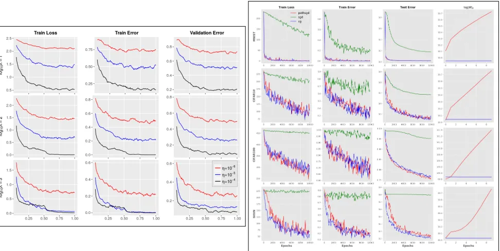
Figure 1: (Left) Performance of CG on ResNet-32 on CIFAR10 dataset (x-axis denotes the fraction ofT): asλincreases, the training error, loss value and test error all start to decrease simultaneously. (Right) Performance of Path-CG vs SGD on a 2-layer fully connected network on four datasets (x-axis denotes the#iterations). Observe that across all datasets, Path-CG is much faster than SGD (first three columns). Last column shows that SGD is not stable with respect to the path norm.
iterates, hence to decrease the effect of random initialization, the training scheme consists of two phases: (i) burn-in phase in which the CG algorithm is run with a constant stepsize; (ii) decay phase in which the stepsize is decaying accord-ing to 1/t. This makes sure that the effect of randomness from the initialization is diminished. We use1epoch for the burn-in phase, hence we can conclude that the algorithm is guaranteed to converge to a stationary point (Lacoste-Julien 2016).
Improve ResNets using Conditional Gradients
We start with the problem of image classification, detection and localization. For these tasks, one of the best perform-ing architectures are variants of the Deep Residual Networks (ResNet) (He and others 2016). For our purposes, to ana-lyze the performance of CG algorithm, we used the shal-lower variant of ResNet, namely ResNet-32 (32 hidden lay-ers) architecture and trained on the CIFAR10 (Krizhevsky, Sutskever, and Hinton 2012) dataset. ResNet-32 consists of5residual blocks and2fully connected, one each at the input and output layers. Each residual block consists of 2 convolu-tion, ReLu (Rectified Linear units), and batch normalization layers, see (He and others 2016) for more details. CIFAR10 dataset contains60000 color images of size32×32with
10different categories/labels. Hence, the network contains approximately0.46Mparameters.
To make the discussion clear, we present results for the case where the total Frobenius norm of the network param-eters is constrained to be less thanλand trained using the CG algorithm. To see the effect of the parametersλand step
sizes η on the model, we ran 80000 iterations, see Figure 1. The plots essentially show that ifλis chosen reasonably big, then the accuracy of CG is very close to the accuracy of ResNet-164 (5.46%top-1 test error, see (He and others 2016)) that hasmany more parameters(approximately 5 times!). In practice, sinceλis a constraint parameter, we can initially chooseλto be small and gradually increase it, thus avoiding complicated grid search procedures.Thus, figure 1 shows that CG can be used to improve the performance of
existing architecturesby appropriately choosing constraints (see supplement for more experiments).
Takeaway:CG offers fewer parameters and higher accu-racy on a standard network with no additional change.
Path-CG vs Path-SGD: Which is better?
In this case study, the goal is to compare Path-CG with the Path-SGD algorithm (Neyshabur, Salakhutdinov, and Srebro 2015) in terms of both accuracy and stability of the algo-rithm. To that end, we considered image classification prob-lem with a path norm constraint on the network:kWtkp ≤λ for varyingλas before. We train a simple feed-forward net-work which consists of2fully-connected hidden layers with
4000units each, followed by the output layer with10nodes. We used ReLu nonlinearity as the activation function and cross entropy as the loss, see (Neyshabur, Salakhutdinov, and Srebro 2015) for more details.
Figure 2:Left:Illustrates the task of image inpainting overall pipeline.Right:CG-trained DC-GAN performs as good as (or better than) SGD-based DC-GAN but with50%epochs.
Figure 3: From left: show MSE/SSIM/FID on thefull im-age.
Figure 1 (right) shows the result forλ = 10−5 (after tun-ing), it can achieve the same accuracy as that of Path-SGD.
Path-CG has one main advantage over Path-SGD: Our results in the supplement show that Path-CG is more sta-ble while the path norm of Path-SGD algorithm increases rapidly. This shows that Path-SGDdoes noteffectively reg-ularize the path norm whereas Path-CG keeps the path norm less thanλas expected.
Takeaway: All statistical benefits of path norm are possi-ble via CG while being computationally stapossi-ble.
Image Inpainting using Conditional Gradients
Finally, we illustrate the ability of our CG framework on an exciting and recent application of image inpainting using Generative Adversarial Networks (GANs). We now briefly explain the overall experimental setup. GANs using game theoretic notions can be defined as a system of 2 neural networks called Generator and the Discriminator competing with each other in a zero-sum game (Arora and others 2017). Image inpainting/completion can be performed using the following two steps (Amos ): (i) Train a standard GAN as a normal image generation task, and (ii) use the trained gener-ator and then tune the noise that gives the best output. Hence, our hypothesis is that if the generator is trained well, then the follow-up task of image inpainting benefits automatically.Train DC-GAN faster for better image inpainting:We used the state of the art DC-GAN architecture in our exper-iments and we impose a Frobenius norm constraint on the
parameters butonlyon the Discriminator to avoid mode col-lapse issues and trained using the CG algorithm. In order to verify the performance of the CG algorithm, we used 2 stan-dard face image datasets from CelebA and LWF and con-ducted two experiments: trained on the CelebA dataset with LFW being the test dataset and vice-versa. We found that the generator generates very high quality images after be-ing trained with LFW images in comparison to the original DC-GANin just10epochs(reducing the computationalcost by50%). Quantitatively, we provide numerical evidence in Figure 3 with2intrinsic metrics viz.,Structural Similarity (SSim), Mean Squared Error (MSE)and1extrinsic met-ric,Frechet Inception Distance (FID). All the three metrics are standard in GAN literature. We calculated the intrinsic metricsafterthe image completion phase. We can see that onall the three metrics, CG outperforms SGD clearly.
Takeaway: GANs can be trained faster with no change in accuracy.
Conclusions
AcknowledgementsThis work is supported by NSF CA-REER RI 1252725 (VS), and UW CPCP (U54 AI117924).
References
Abadi, M., et al. 2016. Tensorflow: Large-scale machine learning on heterogeneous distributed systems.
arXiv:1603.04467.
Amos, B. Image Completion with Deep Learning in Tensor-Flow. http://bamos.github.io/2016/08/09/deep-completion. Accessed: [09/05/2018].
Arora, S., et al. 2017. Generalization and equilibrium in generative adversarial nets (gans). InICML.
Bach, F., et al. 2012. Optimization with sparsity-inducing penalties.Foundations and TrendsR in Machine Learning. Bengio, Y. 2012. Practical recommendations for gradient-based training of deep architectures. In Neural networks: Tricks of the trade.
Boyd, S., and Vandenberghe, L. 2004.Convex optimization. Chambolle, A., and Lions, P.-L. 1997. Image recovery via to-tal variation minimization and related problems. Numerische Mathematik.
Cheng, Y., et al. 2017. A survey of model compression and acceleration for deep neural networks.arXiv:1710.09282. Dauphin, Y.; de Vries, H.; and Bengio, Y. 2015. Equilibrated adaptive learning rates for non-convex optimization. InNIPS. Duchi, J., et al. 2008. Efficient projections onto the l 1-ball for learning in high dimensions. InICML.
Fadili, J. M., and Peyr´e, G. 2011. Total variation projection with first order schemes. IEEE Transactions on Image Pro-cessing.
Frerix, T., et al. 2017. Proximal backpropagation.
arXiv:1706.04638.
Golub, G. H., and Van Loan, C. F. 2012. Matrix computa-tions.
Goodfellow, I.; Bengio, Y.; and Courville, A. 2016. Deep Learning.
Harchaoui, Z.; Juditsky, A.; and Nemirovski, A. 2015. Condi-tional gradient algorithms for norm-regularized smooth con-vex optimization.Mathematical Programming.
Hardt, M.; Recht, B.; and Singer, Y. 2016. Train faster, gener-alize better: Stability of stochastic gradient descent. InICML. He, K., et al. 2016. Deep residual learning for image recog-nition. InCVPR.
Howard, A. G., et al. 2017. Mobilenets: Efficient con-volutional neural networks for mobile vision applications.
arXiv:1704.04861.
Jaggi, M. 2013. Revisiting frank-wolfe: projection-free sparse convex optimization. InICML.
Johnson, R., and Zhang, T. 2013. Accelerating stochastic gradient descent using predictive variance reduction. InNIPS. Krizhevsky, A.; Sutskever, I.; and Hinton, G. E. 2012. Ima-genet classification with deep convolutional neural networks. InNIPS.
Lacoste-Julien, S., and Jaggi, M. 2015. On the global linear convergence of frank-wolfe optimization variants. InNIPS.
Lacoste-Julien, S. 2016. Convergence rate of frank-wolfe for non-convex objectives. arXiv:1607.00345.
M´arquez-Neila, P.; Salzmann, M.; and Fua, P. 2017. Imposing hard constraints on deep networks: Promises and limitations.
arXiv:1706.02025.
Mikolov, T., et al. 2014. Learning longer memory in recurrent neural networks. arXiv:1412.7753.
Netzer, Y., et al. Reading digits in natural images with unsu-pervised feature learning.
Neyshabur, B.; Salakhutdinov, R. R.; and Srebro, N. 2015. Path-sgd: Path-normalized optimization in deep neural net-works. InNIPS.
Neyshabur, B.; Tomioka, R.; and Srebro, N. 2015. Norm-based capacity control in neural networks. InCOLT. Oktay, O., et al. 2017. Anatomically constrained neural net-works (acnn): Application to cardiac image enhancement and segmentation.arXiv:1705.08302.
Pathak, D.; Krahenbuhl, P.; and Darrell, T. 2015. Con-strained convolutional neural networks for weakly supervised segmentation. InICCV.
Platt, J. C., and Barr, A. H. 1988. Constrained differential optimization. InNIPS.
Recht, B.; Fazel, M.; and Parrilo, P. A. 2010. Guaranteed minimum-rank solutions of linear matrix equations via nu-clear norm minimization. SIAM review.
Reddi, S. J., et al. 2016. Stochastic frank-wolfe methods for nonconvex optimization. In54th Annual Allerton Conference. Rissanen, J. 1985.Minimum description length principle. Rudd, K.; Di Muro, G.; and Ferrari, S. 2014. A constrained backpropagation approach for the adaptive solution of partial differential equations. IEEE transactions on neural networks and learning systems.
Ruder, S. 2017. An overview of multi-task learning in deep neural networks. arXiv:1706.05098.
Soudry, D., and Carmon, Y. 2016. No bad local minima: Data independent training error guarantees for multilayer neural networks. arXiv:1605.08361.
Srivastava, N., et al. 2014. Dropout: a simple way to prevent neural networks from overfitting.JMLR.
Tai, C., et al. 2015. Convolutional neural networks with low-rank regularization. arXiv:1511.06067.
Taylor, G., et al. 2016. Training neural networks without gradients: A scalable admm approach. InICML.
Tikhonov, A. N.; Goncharsky, A.; and Bloch, M. 1987. Ill-posed problems in the natural sciences.
Wahba, G. 1990. Spline models for observational data. SIAM.
Yu, Y.; Zhang, X.; and Schuurmans, D. 2017. Generalized conditional gradient for sparse estimation. The Journal of Machine Learning Research.