Matrix Completion for Graph-Based Deep Semi-Supervised Learning

The Thirty-Third AAAI Conference on Artificial Intelligence (AAAI-19)

Matrix Completion for Graph-Based Deep Semi-Supervised Learning

Fariborz Taherkhani, Hadi Kazemi, Nasser M. Nasrabadi

West Virginia University

[email protected], [email protected], [email protected]

Abstract

Convolutional Neural Networks (CNNs) have provided promising achievements for image classification problems. However, training a CNN model relies on a large number of labeled data. Considering the vast amount of unlabeled data available on the web, it is important to make use of these data in conjunction with a small set of labeled data to train a deep learning model. In this paper, we introduce a new iterative Graph-based Semi-Supervised Learning (GSSL) method to train a CNN-based classifier using a large amount of unla-beled data and a small amount of launla-beled data. In this method, we first construct a similarity graph in which the nodes repre-sent the CNN features corresponding to data points (labeled and unlabeled) while the edges tend to connect the data points with the same class label. In this graph, the missing label of unsupervised nodes is predicted by using a matrix comple-tion method based on rank minimizacomple-tion criterion. In the next step, we use the constructed graph to calculate triplet regular-ization loss which is added to the supervised loss obtained by initially labeled data to update the CNN network parameters.

Introduction

CNN models require vast amounts of labeled data to be trained properly; however, providing reliable annotated data to train the CNN models tends to be expensive. There are es-sentially two principal solutions that are usually used to deal with this challenge: 1) Transfer Learning (TL) and 2) Semi-Supervised Learning (SSL). In TL methods (Weiss, Khosh-goftaar, and Wang 2016), we enhance new task learning via transfer of knowledge from a related task which has already been learned. In SSL methods (Zhu 2005), however, we are motivated by the fact that in a lot of applications, there are a vast amount of unlabeled data but only a small amount of labeled data and we essentially aim to learn discriminative learning methods that can make use of the information about the input distribution that is given by a large amount of unla-beled data. The SSL is a broad research field which has been used in variety of applications such as image search (Fergus, Weiss, and Torralba 2009) and natural language processing (Liang 2005). Among the recent SSL approaches, the GSSL methods have received a lot of attention and have become popular due to their flexibility in practical applications and

Copyright c2019, Association for the Advancement of Artificial Intelligence (www.aaai.org). All rights reserved.

low computational complexity. In GSSL methods, one as-sumes that the data points (both labeled and unlabeled) are embedded in a low-dimensional manifold which might be reasonably represented by a graph. In GSSL methods, each data point is expressed as a node in a graph and weights be-tween nodes provide a measure of similarity bebe-tween them. In GSSL, we inject seed labels on a subset of the nodes and then we infer labels on the unlabeled nodes in the graph. The intuition behind the similarity graph is that it captures the information from the labeled samples which is then propa-gated through to the unlabeled samples within the graph.

In this paper, we propose a novel iterative GSSL algo-rithm to train a CNN-based classifier. Our GSSL algoalgo-rithm uses a new method to construct a similarity graph by lever-aging matrix completion method based on rank minimiza-tion criteria. Once the similarity graph is constructed, we use it to regularize the fully supervised loss (i.e., given by initially labeled data points) to force that connected data points in the graph (i.e., data points which belong to the same class) share similar feature representations while dis-connected ones have different representations.

The entire framework is trained end to end such that in each training iteration, the feature representations computed from the CNN are used to construct the similarity graph, then the graph is used to calculate triplet regularization loss which is added to the supervised loss to update the parame-ters of the network which provides new feature representa-tions for the next iteration.

Related Work

trained jointly as in typical GAN framework. The first net-work is a generative model that generates new samples while the other network is the discriminative network. The main problem of this method is training instability, and extra time and memory cost spent to train the two deep networks. Ras-mus et al. (RasRas-mus et al. 2015) merge supervised with unsu-pervised learning methods using a deep learning model. The model is trained to minimize the sum of supervised and un-supervised cost functions by using back propagation, and at the same time prevents the need for layer-wise pre-training. The main problem of this method is the lack of a clear path to generalize it to other network topologies, such as recurrent or residual networks. The probabilistic formulation of CNN models proposed in (Patel, Nguyen, and Baraniuk 2016) na-tively supports SSL introduced by using a new family of hi-erarchical generative models. However, the main concern of these methods is that the activation function requires to be ReLU and that the overall network topology follow a CNN. There are some other methods which extend the generative models for the SSL; for example, Maaløe et al. (Maaløe et al. 2016a) extend GANs with auxiliary variables to learn better variational approximations and more expressive variational distribution. Tobias et al. (Springenberg 2015) propose cate-gorical GAN (CatGAN) which replaces the binary discrim-inator in the standard GAN with a multi-class classifier, and trains the generator and the discriminator using mutal infor-mation on unlabeled samples. Kingma et al. (Kingma et al. 2014) use conditional Variational Autoencoders (VAEs) to treat labels as conditions of generative models to describe the input data; they make posterior inference of labels given unlabeled samples to generate a particular class of samples. Graph-Based Semi-Supervised Learning. The GSSL approaches generally contains two main steps. In the first step, the graph is constructed from all the data points (both labeled and unlabeled data) to represent the relationship be-tween them while in the second step, the information from the labeled data is propagated to the unlabeled data over the graph. Among the different GSSL methods which formulate the information propagation step by using different objec-tive functions such as low-rank minimization (Zheng et al. 2013), k-nearest neighbor methods (Anastasiu and Karypis 2015), structured sparsity (Zhou, Lu, and Peng 2013) min-cut (Blum and Chawla 2001), energy minimization (Blum et al. 2004) and Laplacian spectral method (Fergus, Weiss, and Torralba 2009), there is one common assumption which states that the data points on the same structure (i.e., man-ifold, cluster or subspace) more likely have the same label. In fact, GSSL methods tend to model the structural density among the data points by measuring the proximity (similar-ity) between data points in the graph and then propagate in-formation of labeled data to the unlabeled data in a way that the missing labels in the graph are predicted based on the closest labeled data points (e.g, k-nearest neighbors classi-fier). Since normally there is no explicit solution to model the underlying structures of the data in the feature space, a graph created from the data usually serves as an approxima-tion of the real structure. As a result, constructing a proper graph that best captures the main structure of the data point is important to all GSSL approaches (Berton and de

An-drade Lopes 2015).

Matrix Completion Based on Rank Minimization. The problem of completing a low-rank matrix from a few sam-pled entries has been successfully applied in a variety of applications such as the Netflix challenge. A major break-through by Candes et al. (Cand`es and Recht 2009) states that minimizing a matrix rank subject to some constrains can be recast as minimizing the nuclear norm (sum of singular values) of the matrix. Since nuclear norm minimization of a matrix has characteristic of a Semidefinite Programming (SDP), many approaches have been proposed to solve this minimization problem effectively (Fazel 2002). In the field of computer vision and machine learning, nuclear norm min-imization has been applied to many problems such as robust PCA (Wright et al. 2009) and subspace segmentation (Liu, Lin, and Yu 2010).

Similarity Graph Construction

In this section, we describe our method to construct the similarity graph via the matrix completion method. Let g(x1), ..., g(xn) ∈ Rd be the features captured by the

CNN model corresponding tonsamples; each of these sam-ples is represented by a node in the similarity graph. Let X= [g(x1), g(x2), ..., g(xn)]be ad×nfeature matrix

con-structed by stacking samples column wise. Suppose thatcis the number of classes;y1, ..., ynare one hot encoding label

of samples, andY= [y1, ..., yn]indicates ac×nlabel

ma-trix which is obtained by a linear model fromX(i.e.,yi =

Wg(xi) +b, whereWis ac×nweight matrix). In our

prob-lem, all the entries in feature matrixXare known and ob-servable; however, entries corresponding to unlabeled sam-ples in the label matrixYare missed and we essentially aim to predict them. We note that by assumingXas a low rank matrix, the combined(c+d)×nmatrixZ= [X;Y]produces a low rank matrix too (i.e., rank([X;Y])≤rank(X)+c); and predicting the missing entries in this matrix can be cast as a matrix completion problem (Cai, Cand`es, and Shen 2010; Cabral et al. 2011). Here, we take advantage of the matrix completion method to predict missing labels in the graph.

which minimizes the nuclear norm ||Z||∗ = Pnk=1σk(Z)

(the sum of the singular values) under the constraint set over the observed entries; whereσk(Z)denotes the kth largest

singular value ofZ. The nuclear norm of matrixZis the dual norm of the spectral norm of the matrixZwhich is convex, and it can be solved by variety of convex optimization al-gorithms (Fazel 2002). The relationship between rank and nuclear norm is similar to that of`0norm and`1norm for

vectors. Since we can not minimize the rank of the matrix, we choose the nuclear norm as an alternative optimization problem which is the tightest convex relaxation to the rank.

Predicting Missing Labels via Matrix Completion

In this section, we provide an optimization problem to pre-dict missing entries of the data matrixZ= [X;Y]such that the nuclear norm ofZis minimized and entries inZmatch the observed entries ( i.e., labels of supervised data and fea-ture matrixX). LetΩXbe the index set of observed entries

in the feature matrixX, where(i, j)∈ΩXif and only ifXij

is observed. Likewise, letΩY be the index set of observed

entries in the label matrixYand(i, j)∈ ΩYif and only if

yj is a labeled sample. In this problem|ΩX| = d×n( no

missing entries inX), and1 <|ΩY| < c×n(some

miss-ing entries inY). The optimization problem for predicting missing entries inZis defined as follow:

argmin

Z

µ||Z||∗+

1

|ΩX|

X

i,j∈ΩX

cx(zij, xij)+

λ

|ΩY|

X

i,j∈ΩY

cy(z(i+d)j, yij).

(1)

We shift row index of the stacked matrix Z in the cy(z(i+d),j, yij) because we want to skip X part in the

Z. Apart from minimizing the nuclear norm ofZ, we pe-nalize the cost function in (1) by adding cy(.) and cx(.)

losses to avoid trivial solutions and large distortions of Z from the observed entries in X and Y matrices. The served label data type is of a different type than the ob-served feature data; thus we define two different losses. The cx(zij, xij) = ₂1(zij−xij)2is defined as the squared loss,

while the cy(z(i+d)j, yij) = log(1 + exp(−z(i+d)j.yij))

is the logistic loss which accentuates the error on entries switching labels as is different from their absolute numerical deviation. The parametersµ, λare the weights which create a balance between errors for better label error correction and feature adaptation.

Optimization Method The loss defined in (1) is a con-vex optimization problem. We use the soft-impute algorithm (Mazumder, Hastie, and Tibshirani 2010) which is a simple and effective algorithm for nuclear norm regularized matrix completion. This algorithm iteratively restore the missing entries with those attained from a soft-thresholded SVD. We first define a projection operatorPΩon the observed setΩ

as follows:

[PΩ(Z)]ij =

zij (i, j)∈Ω

0 (i, j)6∈Ω (2)

thus, the optimization problem in (3) can be rewritten as fol-lows:

f(Z) =µ||Z||∗ | {z } G(Z)

+ 1 2|ΩX|

||PΩ(X)−PΩ(Zx)||2F

| {z }

H(Zx)

+

λ

|ΩY|

log(1 +exp(−PΩ(Zy)◦PΩ(Y)))

| {z }

U(Zy)

, (3)

where, Zx andZy are sub-matrices ofZ for parts Xand

Y, respectively (i.e.,Z = [X;Y]), and symbol◦ indicates Hadamard or element wise product between PΩ(Zy) and

PΩ(Y). In this set of formulation, we call the second and

third parts H(Zx), U(Zy), respectively which are convex

and smooth, and the first partG(Z)which is also convex but not smooth. Therefore, we can think about three ingredients needed for proximal gradient descent:

•The first is∇H(Zx); here subgradient is just the

gradi-ent:

∇H(Zx) =−

1

|ΩX|

(PΩ(X)−PΩ(Zx)), (4)

where, the gradient ofH(zij)is−_|Ω1

X|(xij−zij).

• The second is∇U(Zy); here, subgradient is also just

the gradient:

∇U(Zy) =

λ

|ΩY|

−PΩ(Y)

1 +exp(PΩ(Zy)◦PΩ(Y))

, (5)

where, the gradient ofU(z(i+d)j)is|ΩλY|

−yij

1+exp(z(i+d)jyij).

•The third is theproxoperator:

proxt(Z) =arg min

C

1

2t||Z−C||

2

F+µ||C||∗. (6)

It can be proved that proxt(Z) = Sλt(Z) (Mazumder,

Hastie, and Tibshirani 2010) which is thematrix soft thresh-olding at the levelλ; whereSλ(Z)is defined by

Sλ(Z) =UΣλV>, (7)

where,Z = UΣλV> is an SVD, and Σλ is diagonal with

(Σλ)ii = max{Σii−λ,0}. This matrix soft-thresholding

is an element-wise soft-thresholding of the matrix. By using a soft-threaded singular matrixΣλ, this returns a low-rank

proxresult.

Therefor, the Proximal Gradient update step is written as follows:

Z+=proxt(Z−t(∇H(Zx) +∇U(Zy)))

=Sλt(Z−t(∇H(Zx) +∇U(Zy)).

(8)

Note that (∇H(Zx) +∇U(Zy)) is Lipschitz continuous

withL = 1, thus we can choose fixed step sizet = 1and then the update step in this case is expressed as follows:

Z+=Sλ(Z−(∇H(Zx) +∇U(Zy)). (9)

Supervised Task Regularization via the

Constructed Graph

In this section, we provide a new approach based on the triplet loss function to leverage the constructed graph for training the CNN model. In this approach, we aim to reg-ularize the supervised task by adding a semi-supervised loss term as an auxiliary task to the CNN. In other words, we concentrate mostly on the classifier regularization learned in a supervised fashion with few labeled data. To regularize the supervised task using unsupervised data, we apply the triplet loss function using a triplet of data on the graph as follows;

Ltrip(g(xa), g(xp), g(xn), A) =

max(||g(xa)−g(xp)||2− ||g(xa)−g(xn)||2+α,0),

(10) whereAis the adjacency matrix of the graph in which en-tries in the matrix indicate if pairs of the nodes are adjacent or not in the graph; the α parameter is the margin in the triplet loss andg(xa), g(xp), g(xn)are the output of CNN

for the imagesxa, xpandxn, respectively. In triplet loss, we

look at the three data point on the graph at the same time; in our case we choose labeled samples in the graph as the anchor (i.e., samplexain (10)) and samplexpas a positive

sample ifA(xa, xp) = 1and samplexnas a negative

sam-ple ifA(xa, xn) = 0; we want to bring positive and anchor

pairs (i.e., two images which are connected in the graph) close to each other while push away the negative and anchor pairs (i.e., two images which are not connected in the graph) simultaneously. The triplet loss is added to the total network loss function to regularize the supervised classification loss with an auxiliary semi-supervised loss term.

Deep Semi Supervised Loss Function

Now, we have all the loss terms including the supervised loss and semi-supervised loss to set up the total CNN loss function. Our SSL loss function for updating the CNN pa-rameters is defined as follows:

L(w,x,y) = X

xi∈xs

Lc(w, g(xi), yi)

| {z }

supervised

+

γ X

xa∈xs;{xp,xn}∈x

Ltrip(w, g(xa), g(xp), g(xn), A)

| {z }

semi-supervised

!

,

(11) wherex andy are the training batch and samples labels in the training batch (i.e., real labels and predicted labels);

Lcis supervised classification loss (softmax loss is used, but

can be chosen other type of losses such as center loss, con-trastive center loss);xsis the supervised samples in training

batchx. Thewis the parameters of the CNN andγis the balancing term between two supervised and semi-supervised losses. The batch set is created such that number of similar (i.e., anchor and positive) and dissimilar (i.e., anchor and negative) pairs to be roughly balanced. In each triplet, the labeled data (not predicted labels) are chosen as the anchor

and predicted labeled data are considered only as positive and negative samples in the batch.

Experiments

Datasets and Pre-Processing. We conducted our experi-ments on the widely used MNIST (LeCun et al. 1998), SVHN (Netzer et al. 2011), small NORB (LeCun, Huang, and Bottou 2004) and CIFAR 10 (Krizhevsky and Hinton 2009) datasets. For each of these datasets, we split the train-ing set to two different sets of labeled and unlabeled sam-ples. We ensure that all the classes are balanced such that each class should have the same number of labeled samples. We ran our model for 10 times with different random splits of the labeled and unlabeled data for each dataset, and we report the mean and standard deviation of the error rate.

MNIST is handwritten digits of 10 different classes dataset which contains a training set of 60,000 samples, and a test set of 10,000 samples. The digits have been size-normalized and centered in a fixed-size (28×28) images. We select 100 samples in the training set as labeled and re-maining of it as unlabeled.

SVHN is another digit dataset similar to MNIST with 32×32color images centered around a single character. The task is to classify the center digits in the images; we follow (Sermanet, Chintala, and LeCun 2012; Goodfellow et al. 2013) methods to split the dataset to 598,388 train-ing data and 26,032 testtrain-ing data. For this dataset, we choose randomly 1000 samples as labeled and rest of it, is used as unlabeled.

CIFAR-10is a collection of32×32RGB images of 10 classes including airplane, automobile, bird, cat, deer, dog, frog, horse, ship and trucks. This dataset contains 50,000 number of images for training and 10,000 for testing; we select 4,000 samples in the training set as labeled and rest as unlabeled.

NORB contains gray scale images of 5 general classes including animal, human, airplane, truck and car. The ob-jects were imaged by two cameras under different lighting conditions, elevations and azimuths. This dataset contains 24,300 images for both training and testing sets. In our ex-periments, we resize the images to32×32as it is in (Maaløe et al. 2016b); we select 1,000 samples in the training set as labeled and remaining is considered as unlabeled.

Figure 1: The labels of unsupervised nodes in the graph are predicted and then the graph is used to train the network.

Methods MNIST(100) SVHN(1000) NORB(1000) CIFAR-10(4000) Matrix Completion 1.98(±0.03) 10.06(±0.08) 9.11(±0.11) 19.91(±0.23)

GSCNN+No Reg 1.14(±0.09) 8.41(±0.22) 8.71(±0.18) 18.03(±0.31) GSCNN 0.84(±0.12) 5.13(±0.39) 7.01(±0.53) 15.49(±0.64)

Table 1: Comparing GSCNN error rate in different scenarios on MNIST, SVHN, NORB and CIFAR-10 datasets.

(a) (b)

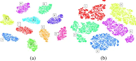
Figure 2: Visualizations of training data which are partially labeled for (a) MNIST and (b) NORB datasets using our GSSL method.

potentially helps to achieve faster learning as well as higher overall accuracy. Furthermore, batch normalization allows us to use a higher learning rate, which potentially provides another boost in speed. The parameters of the network are initialized by sampling randomly fromN(0,0.001)except for the bias parameters which are initialized as zero. We im-plemented our framework in TensorFlow and performed our experiments on two GeForce GTX TITAN X 12GB GPUs. We use Adam optimizer (Kingma and Ba 2014) with the default hyper-parameters values ( = 10−3 , β1 = 0.9,

β2= 0.999) in our experiments. The batch size in all

exper-iments is fixed to 128, and we setγto 0.1 experimentally to create a balance between supervised loss and unsupervised loss in the total network loss function.

Hyper-Parameter Tuning.We used 10-fold cross vali-dation in each experiment to tune hyper-parameters in our model. For λin (1), we randomly divide the labeled data into ten disjoint subsets; next we run the matrix comple-tion over ₁₀9 and we calculate the performance on the re-maining ₁₀1; then we average the results over the 10 folds (We note that we used label error as performance criterion to select parameters because our goal in MC is to predict

label of unlabeled data points). The range ofλ values are

{10−3,10−2,10−1,1}. For µin (1), we initialize it to be 0.25σ1, whereσ1is the largest singular value of the matrix

[X;Y]and decrease it gradually until10−5as it is suggested in (Mazumder, Hastie, and Tibshirani 2010).

Matrix Completion.We use SoftImput algorithm imple-mented in fancyimput package in python to predict missing labels in the graph. We set shrinkage value which is the value by which we shrink singular values on each iteration to the maximum singular value of the initialized matrix (zeros for missing values) divided by 100; the maximum number of SVD iteration is set to 1000. In matrix completion, we stop the algorithm by defining a convergence threshold (0.001 in our experiments) which is the minimum ration difference be-tween iterations (as a fraction of the Frobenius norm of the current solution). In SoftImput algorithm, a sequence of so-lutions are produced for which the criterion decreases to the optimal solution with every iteration. Convergence thresh-old can be given to the SoftImput algorithm implemented in fancyimput package.

Triplet Mining on the Graph. In our experiments, we concentrate on the online triplet mining strategy to gen-erate useful triplets for data on the graph. Considering a batch ofbsamples, we extract CNN features for each sam-ple, and we then can create a maximum ofb3_{triplets even}

though most of these triplets are not valid (i.e., triplet ex-cept two positive and one negative). This technique pro-vides us more triplets for a single batch of samples during the network training. We use all the valid triplets in the training and we average the loss on the hard triplet (i.e., d(g(xn), g(xa) < d(g(xp), g(xa))) and semi-hard triplet

(i.e.,d(g(xa), g(xp))< d(g(xa), g(xp)) +α); we disregard

the easy triplets ( triplets with zero loss) because averaging on them makes the overall loss very small.

Samples Per Class 100 200 400 800 NORB 9.88(±0.54) 7.01(±0.53) 6.12(±0.41) 5.07(±0.19) CIFAR-10 18.98(±0.62) 16.82(±0.47) 15.49(±0.64) 14.51(±0.34)

Table 2: GSCNN error rate by given number of initially labeled data per class. Results are averaged on 10 times randomly split.

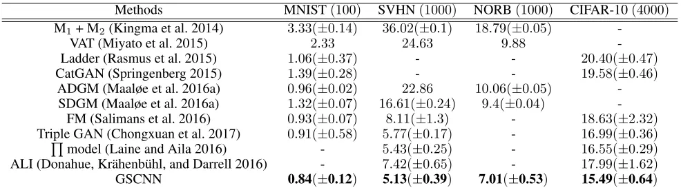
Methods MNIST(100) SVHN(1000) NORB(1000) CIFAR-10(4000) M1+ M2(Kingma et al. 2014) 3.33(±0.14) 36.02(±0.1) 18.79(±0.05)

-VAT (Miyato et al. 2015) 2.33 24.63 9.88

-Ladder (Rasmus et al. 2015) 1.06(±0.37) - - 20.40(±0.47) CatGAN (Springenberg 2015) 1.39(±0.28) - - 19.58(±0.46)

ADGM (Maaløe et al. 2016a) 0.96(±0.02) 22.86 10.06(±0.05) -SDGM (Maaløe et al. 2016a) 1.32(±0.07) 16.61(±0.24) 9.4(±0.04)

-FM (Salimans et al. 2016) 0.93(±0.07) 8.11(±1.3) - 18.63(±2.32) Triple GAN (Chongxuan et al. 2017) 0.91(±0.58) 5.77(±0.17) - 16.99(±0.36)

Q

model (Laine and Aila 2016) - 5.43(±0.25) - 16.55(±0.29) ALI (Donahue, Kr¨ahenb¨uhl, and Darrell 2016) - 7.42(±0.65) - 17.99(±1.62) GSCNN 0.84(±0.12) 5.13(±0.39) 7.01(±0.53) 15.49(±0.64)

Table 3: Comparing SSL models on MNIST, SVHN, NORB and CIFAR-10 datasets

which indicates the case where we remove the triplet regu-larization loss in (11) and use all the labeled and unlabeled data with true and completed labels directly in the softmax classifier loss, b) GSCNN which indicates the case where we use the triplet regularization loss in (11) in training of our CNN model. Table.1 shows the performance of our model in two different scenarios (i.e., a) GSCNN+No Reg and b) GSCNN); the results show that our regularization loss based on the triplet can improve the model performance by 0.3%, 3.28%, 1.7% and 2.54% on the MNIST, SVHN, NORB and CIFAR-10 datasets, respectively. This improvement is be-cause the softmax classifier loss only forces the CNN fea-tures of different classes to stay apart, while the triplet loss not only does this, but also efficiently brings the CNN fea-tures of the same class close to each other. Therefore, by considering triplet regularization in the training, not only the inter-class features differences are enlarged, but also the intra-class features variations are reduced. Moreover, since our method is an iterative process of two steps (i.e., the first step uses matrix completion to predict the labels, and the next step uses the predicted results to train a CNN), we re-ported in Table.1 the matrix completion error rates to pro-vide an empirical analysis showing that matrix completion has significant influence on training the CNN model. Accu-racy of the matrix completion indicates those unlabeled data predicted correctly by matrix completion, are then used in the regularizer to improve the CNN performance.

Constructed Graph Properties. The graph in our model is constructed dynamically while the CNN network is trained; this is because the graph in our model needs the network output to be constructed. In our SSL method, the graph is created online in a local scope (over a few samples of training set) which is virtually similar to the concept of training batch in the CNN models. In each training batch, the labels of the unsupervised data are predicted based on all the labeled data using our matrix completion method. In-deed, we take a batch of training data and then we predict the

class label of unsupervised data to construct the graph for the batch. Our graph construction method is an Expectation Maximization (EM) like algorithm in a sense that in forward pass, the graph is constructed for a batch (including labeled and unlabeled data), and later on it is used as a regularizer in the network loss calculation to update the network parame-ters by back propagation in the backward pass. This property enables us to create a robust graph through the training step; because the graph is constructed by better set of CNN fea-tures as we train the CNN through several training epochs. This factor makes the graph construction method more ro-bust in comparison to the offline based graph construction methods with static data embedding.

Most of graph construction algorithms are usually expen-sive in terms of time complexity. For example, graph con-struction using offlinek-NN method in brute-force fashion isO(n2_{)wherenis number of training data. Even though}

there are other efficient methods (Zhang et al. 2013) to im-provek-NN method in terms of time complexity, in most of the offline construction methods the time complexity usu-ally makes graph construction step unpractical speciusu-ally for the large scale datasets. However, splitting the data to small chunks of data with equal size which in our case is the batch makes the graph construction step more efficient, and also feasible for online computation and simultaneous with CNN training; because in this case, only a small portion of the training data is used to construct the graph. Our method is online and use small part of the whole data. The computa-tionally demanding part of our graph construction algorithm is the equation (9) where we take SVD from a low-rank ma-trixZto predict missing label of unsupervised nodes in the graph. For example, it takes around 6 (secs) to complete a 100×100 matrix in each iteration of our algorithm.

(a)

(b)

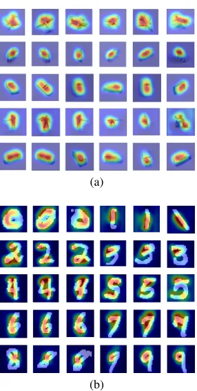
Figure 3: Example of Grad-CAM generated for (a) NORB and (b) MNIST datasets from our GSSL; it is shown that highlighted regions are activated by Grad-CAM algorithm for different classes.

labeled data points on the final performance. In this exper-iment, we selected 100 samples per each class and grad-ually increased the number of samples to 200, 400, and 800, respectively; the results in Table.2 indicate that the model performance increases as the number of initially la-beled data points in the regularizer increases. The trend of improvement is reported in Table.2. The results on the CIFAR-10 dataset show the model is improved by around 2.16%, 1.33% and 0.98% when we increase the number of labeled samples from 100 −→ 200 , 200 −→ 400 and 400 −→ 800, respectively, while on the NORB dataset, the model performance is improved by around 2.87%, 0.89% and 1.05% when we increase the number of labeled samples from100−→200,200−→400and400−→800, respectively. Evaluation and Discussion. We compare our GSSL model with a large body of previous models on MNIST, SVHN, NORB and CIFAR-10 datasets using 100, to , 4000labeled samples, respectively. Experimental results in Table.3 show that our method is competitive to the state-of-the-art results for all these datasets; given 100 labeled samples on the MNIST dataset, our method still is com-parable to the outstanding generative models including FM (Salimans et al. 2016) and Triplet GAN (Chongxuan et al. 2017); Table.3 also shows Semi-Supervised results on the more challenging datasets including SVHN, NORB and CIFAR-10 datasets. Following previous models (Maaløe et al. 2016a; Kingma et al. 2014; Miyato et al. 2015), we use

1,000 labeled samples on SVHN and NORB datasets to compare our method with other methods. The results show that our method outperforms the previous state-of-the-art.

Inspired by the Grad-CAM (Selvaraju et al. 2016) on class activation map, we can interpret the classification decision made by our method. We can see that our model is trig-gered by different semantic regions of the image for different classes of classification. Fig. 3 shows that our GSSL method by using Grad-CAM method provides ”visual explanations” for decisions from the all classes of the CNN models. The Fig. 3 indicate the class activation of the model for MNIST and NORB dataset where we use 100 and 1,000 labeled samples to train the model and use the remaining as test; the result shows the outstanding result of the model in object lo-calization using Grad- CAM technique. We also used T-SNE (Maaten and Hinton 2008) to visualize the CNN features for training data which are partially supervised. Fig. 2 indicates that the model has acceptable discriminative ability; we ap-plied this method on MNIST and NORB datasets using 100 and 1,000 labeled samples in the training step. The figure shows that our model can discriminate the training data in the embedded space using partially supervised samples.

Conclusion

In this paper, we proposed a new Graph-based Semi-Supervised Learning method to train a CNN model using a vast amount of unsupervised data in conjunction with a small amounts of supervised data. In this model, we make structural assumption about the data point to predict the missing labels on the graph and then we leverage the con-structed graph as regularizer to train the CNN model. Ex-perimental results show that our model is comparable to the state of the art for Semi-Supervised image classification.

References

Anastasiu, D. C., and Karypis, G. 2015. L2knng: Fast exact k-nearest neighbor graph construction with l2-norm prun-ing. InProceedings of the 24th ACM International on Con-ference on Information and Knowledge Management, 791– 800. ACM.

Arjovsky, M.; Chintala, S.; and Bottou, L. 2017. Wasserstein gan. arXiv preprint arXiv:1701.07875.

Berton, L., and de Andrade Lopes, A. 2015. Graph construc-tion for semi-supervised learning. InIJCAI, 4343–4344. Blum, A., and Chawla, S. 2001. Learning from labeled and unlabeled data using graph mincuts.

Blum, A.; Lafferty, J.; Rwebangira, M. R.; and Reddy, R. 2004. Semi-supervised learning using randomized mincuts. In Proceedings of the twenty-first international conference on Machine learning, 13. ACM.

Cabral, R. S.; Torre, F.; Costeira, J. P.; and Bernardino, A. 2011. Matrix completion for multi-label image classifica-tion. In Advances in Neural Information Processing Sys-tems, 190–198.

Cand`es, E. J., and Recht, B. 2009. Exact matrix comple-tion via convex optimizacomple-tion.Foundations of Computational mathematics9(6):717.

Chistov, A. L., and Grigor’Ev, D. Y. 1984. Complexity of quantifier elimination in the theory of algebraically closed fields. InInternational Symposium on Mathematical Foun-dations of Computer Science, 17–31. Springer.

Chongxuan, L.; Xu, T.; Zhu, J.; and Zhang, B. 2017. Triple generative adversarial nets. InAdvances in Neural Informa-tion Processing Systems, 4091–4101.

Donahue, J.; Kr¨ahenb¨uhl, P.; and Darrell, T. 2016. Adver-sarial feature learning.arXiv preprint arXiv:1605.09782. Fazel, M. 2002.Matrix rank minimization with applications. Ph.D. Dissertation, PhD thesis, Stanford University. Fergus, R.; Weiss, Y.; and Torralba, A. 2009. Semi-supervised learning in gigantic image collections. In Ad-vances in neural information processing systems, 522–530.

Goodfellow, I. J.; Warde-Farley, D.; Mirza, M.; Courville, A.; and Bengio, Y. 2013. Maxout networks. arXiv preprint arXiv:1302.4389.

Kingma, D. P., and Ba, J. 2014. Adam: A method for stochastic optimization.arXiv preprint arXiv:1412.6980.

Kingma, D. P.; Mohamed, S.; Rezende, D. J.; and Welling, M. 2014. Semi-supervised learning with deep generative models. InAdvances in Neural Information Processing Sys-tems, 3581–3589.

Krizhevsky, A., and Hinton, G. 2009. Learning multiple layers of features from tiny images.

Laine, S., and Aila, T. 2016. Temporal ensembling for semi-supervised learning. arXiv preprint arXiv:1610.02242. LeCun, Y.; Bottou, L.; Bengio, Y.; and Haffner, P. 1998. Gradient-based learning applied to document recognition. Proceedings of the IEEE86(11):2278–2324.

LeCun, Y.; Huang, F. J.; and Bottou, L. 2004. Learning methods for generic object recognition with invariance to pose and lighting. InComputer Vision and Pattern Recogni-tion, 2004. CVPR 2004. Proceedings of the 2004 IEEE Com-puter Society Conference on, volume 2, II–104. IEEE. Liang, P. 2005. Semi-supervised learning for natural lan-guage. Ph.D. Dissertation, Massachusetts Institute of Tech-nology.

Liu, G.; Lin, Z.; and Yu, Y. 2010. Robust subspace seg-mentation by low-rank representation. InProceedings of the 27th international conference on machine learning (ICML-10), 663–670.

Maaløe, L.; Sønderby, C. K.; Sønderby, S. K.; and Winther, O. 2016a. Auxiliary deep generative models.arXiv preprint arXiv:1602.05473.

Maaløe, L.; Sønderby, C. K.; Sønderby, S. K.; and Winther, O. 2016b. Auxiliary deep generative models.arXiv preprint arXiv:1602.05473.

Maaten, L. v. d., and Hinton, G. 2008. Visualizing data using t-sne. Journal of machine learning research9(Nov):2579– 2605.

Mazumder, R.; Hastie, T.; and Tibshirani, R. 2010. Spectral regularization algorithms for learning large incomplete ma-trices.Journal of machine learning research11(Aug):2287– 2322.

Miyato, T.; Maeda, S.-i.; Koyama, M.; Nakae, K.; and Ishii, S. 2015. Distributional smoothing with virtual adversarial training. arXiv preprint arXiv:1507.00677.

Netzer, Y.; Wang, T.; Coates, A.; Bissacco, A.; Wu, B.; and Ng, A. Y. 2011. Reading digits in natural images with unsu-pervised feature learning. InNIPS workshop on deep learn-ing and unsupervised feature learnlearn-ing, volume 2011, 5. Patel, A. B.; Nguyen, M. T.; and Baraniuk, R. 2016. A probabilistic framework for deep learning. InAdvances in neural information processing systems, 2558–2566. Rasmus, A.; Berglund, M.; Honkala, M.; Valpola, H.; and Raiko, T. 2015. Semi-supervised learning with ladder net-works. InAdvances in Neural Information Processing Sys-tems, 3546–3554.

Salimans, T.; Goodfellow, I.; Zaremba, W.; Cheung, V.; Rad-ford, A.; and Chen, X. 2016. Improved techniques for train-ing gans. In Advances in Neural Information Processing Systems, 2234–2242.

Selvaraju, R. R.; Cogswell, M.; Das, A.; Vedantam, R.; Parikh, D.; and Batra, D. 2016. Grad-cam: Visual expla-nations from deep networks via gradient-based localization. See https://arxiv. org/abs/1610.02391 v37(8).

Sermanet, P.; Chintala, S.; and LeCun, Y. 2012. Convolu-tional neural networks applied to house numbers digit clas-sification. InPattern Recognition (ICPR), 2012 21st Inter-national Conference on, 3288–3291. IEEE.

Springenberg, J. T. 2015. Unsupervised and semi-supervised learning with categorical generative adversarial networks. arXiv preprint arXiv:1511.06390.

Weiss, K.; Khoshgoftaar, T. M.; and Wang, D. 2016. A survey of transfer learning. Journal of Big Data3(1):9. Wright, J.; Ganesh, A.; Rao, S.; Peng, Y.; and Ma, Y. 2009. Robust principal component analysis: Exact recovery of cor-rupted low-rank matrices via convex optimization. In Ad-vances in neural information processing systems, 2080– 2088.

Zhang, Y.-M.; Huang, K.; Geng, G.; and Liu, C.-L. 2013. Fast knn graph construction with locality sensitive hashing. In Joint European Conference on Machine Learning and Knowledge Discovery in Databases, 660–674. Springer. Zheng, Y.; Zhang, X.; Yang, S.; and Jiao, L. 2013. Low-rank representation with local constraint for graph construction. Neurocomputing122:398–405.