The Thirty-Third AAAI Conference on Artificial Intelligence (AAAI-19)
Efficient Data Point Pruning for One-Class SVM
Yasuhiro Fujiwara,
†‡\Sekitoshi Kanai,
†Junya Arai,
†Yasutoshi Ida,
†Naonori Ueda
‡]†NTT Software Innovation Center, 3-9-11 Midori-cho Musashino-shi, Tokyo, 180-8585, Japan
‡NTT Communication Science Laboratories, 2-4 Seika-Cho Soraku-gun, Kyoto, Japan
\Osaka University, 1-5 Yamadaoka, Suita-shi, Osaka, Japan
]RIKEN Center for AIP, 1-4-1 Nihonbashi, Chuo-ku, Tokyo, 103-0027, Japan
{fujiwara.yasuhiro, kanai.sekitoshi, arai.junya, ida.yasutoshi, ueda.naonori}@lab.ntt.co.jp
Abstract
One-class SVM is a popular method for one-class classifica-tion but it needs high computaclassifica-tion cost. This paper proposes
Quixas an efficient training algorithm for one-class SVM.
It prunes unnecessary data points before applying the SVM solver by computing upper and lower bounds of a parame-ter that deparame-termines the hyper-plane. Since we can efficiently check optimality of the hyper-plane by using the bounds, it guarantees the identical classification results to the original
approach. Experiments show that it is up to6800times faster
than existing approaches without degrading optimality.
Introduction
Due to the rapid development of Internet and database tech-nologies, we can improve the effectiveness of applications by using knowledge from big data (Fujiwara et al. 2017a; Mishima and Fujiwara 2015; Nakatsuji and Fujiwara 2014). Machine learning approaches play important role in ex-tracting knowledge from big data (Fujiwara et al. 2017b; Tanaka et al. 2016; Nakatsuji et al. 2014). One-class SVM is a popular machine learning approach to achieving one-class one-classification (Sch¨olkopf et al. 2001). It computes a hyper-plane that separates data points of the target class. Data points are called support vectors if they are representa-tive of the hyper-plane, and they are called outliers if they are not labeled as the target class. One-class SVM offers the ad-vantage of the desirable properties of traditional SVMs. For instance, it has a unique solution in computing the hyper-plane since its optimization problem is convex. However, its computation cost is excessive especially for large-scale data since it needs to solve a quadratic programming prob-lem withnconstraints wherenis the number of data points. The shrinking approach is a popular method to reduce the computation cost of SVM (Joachims 1999). Although it can compute the optimal hyper-plane, it needs high computa-tion cost in checking the optimality. The Nystr¨om method approximates a kernel matrix used in the solver by select-ing data points as landmarks (Drineas and Mahoney 2005). Specifically, it computes a small matrix of landmarks where all data points are projected by using kernel similarities be-tween landmarks and data points. Random Fourier features
Copyright c2019, Association for the Advancement of Artificial
Intelligence (www.aaai.org). All rights reserved.
can reduce the computational cost of SVM by constructing a random mapping into a low-dimensional feature space for kernel functions (Rahimi and Recht 2007). However, these approaches need the high computation cost since they apply the solver to all the data points. Note that, since the origi-nal approaches of the Nystr¨om method and random Fourier features use simple algorithms (Drineas and Mahoney 2005; Rahimi and Recht 2007), they are more effective in reduc-ing computation cost comparreduc-ing to the recent approaches of the Nystr¨om method and random Fourier features (Li et al. 2016; Musco and Musco 2017; Wu et al. 2016). Noumir et al. proposed an online learning approach based on the coherence criterion (Noumir, Honeine, and Richard 2012). The approach computes the hyper-plane by updating the Gram matrix and its inverse matrix by exploiting the Wood-bury matrix identity. In terms of efficiency, this approach outperforms the adaptive approach (G´omez-Verdejo et al. 2011). Gao proposed the active-set method based online ap-proach for one-class SVM to improve the efficiency (Gao 2015). It applies the solver to data points only if their dis-tance to the center of the hyper-plane is not less than the ra-dius of the hyper-plane. However, they can erroneously re-move data points that are actually support vectors for the optimal hyper-plane; they sacrifice the optimality of the hyper-plane to increase the efficiency. Note that there ex-ists a gap between the performance of approximate and the optimal approaches in terms of accuracy (Li et al. 2016; Fujiwara et al. 2015; 2013; Yang et al. 2012).
Preliminaries
In one-class SVM, vectorxi= (xi[1],xi[2],. . . ,xi[m]) cor-responds to thei-th data point inmdimensional space and can be represented as thei-th row vector of data matrixX
whose column vectors are standardized (C¸ eker and Upad-hyaya 2016; Fisher, Camp, and Krzhizhanovskaya 2016). Letw,ξi, andρbe anm-dimensional vector, a slack vari-able, and an offset, respectively, it solves the following quadratic programming problem:
min
w∈F,ξ∈Rn,ρ∈R
1
2kwk
2+ 1
nν
Pn
i=1ξi−ρ (1)
Subject to (w·Φ(xi))≥ρ−ξi,ξi ≥0 (2)
In Equation (2),Φis a kernel map X → F which trans-forms the training data points into a high-dimensional fea-ture space. We have the following dual problem by intro-ducing the Lagrange function:
min
α 1 2
Pn
i,j=1αiαjK(xi,xj) (3)
subject to0≤αi≤nν1 ,P n
i=1αi= 1 (4) Here, α is a vector whose i-th elementαi is a Lagrange multiplier of data pointxi, andK(xi,xj)is a kernel func-tion such as the Gaussian kernel given as e−γkxi−xjk2
. In Equation (3), the data points that have αi > 0 and αi = nν1 are called support vectors and outliers, respec-tively, andνis a lower bound of the fraction of support vec-tors and an upper bound on the fraction of outliers. This in-dicates that training accuracy should be at least1−ν. Let
z=Pn
i=1αiK(x,xi)−ρbe a parameter for data pointx, the decision function is given as follows:
f(x) = sgn(z) = sgn(Pn
i=1αiK(x,xi)−ρ) (5) Since the dual problem is convex, we can compute the op-timal hyper-plane by applying the solver. We can compute offsetρasρ=Pn
i=1αiK(xi,xj)wherexjis the data point for which0< αj <nν1 .
However, one-class SVM has a drawback; its computation cost is high in obtaining the hyper-plane. This is because it needs to solve a quadratic programming problem withn
constraints. Even though Sequential Minimal Optimization (SMO) is known to be an efficient SVM solver to obtain the optimal hyper-plane, its computation cost is quadratic to the number of data points.
Proposed method
Main ideas
The original algorithm applies the solver to all data points. Our approach exploits the property of one-class SVM that the hyper-plane is determined only by support vectors (Sch¨olkopf et al. 2001); we select data points to apply the solver by upper and lower bounds of parameterz.
This approach has several advantages. First, the hyper-plane obtained by our approach is guaranteed to be op-timal unlike the previous approaches for SVM (Drineas and Mahoney 2005; Gao 2015; G´omez-Verdejo et al. 2011; Noumir, Honeine, and Richard 2012; Rahimi and Recht
2007). This is because our approach checks whether the ob-tained hyper-plane is theoretically identical to the optimal hyper-plane by exploiting the upper and lower bounds. Sec-ond, our approach can efficiently check the optimality of the hyper-plane since we can efficiently compute the bounds used in the optimality check. Although the shrinking ap-proach selects data points similar to our apap-proach, it needs high computation cost to check the optimality of the hyper-plane by computing kernel functions (Joachims 1999). Ifs
is the number of support vectors, the shrinking approach re-quiresO(snm)time while our approach needs at mostO(n) time in checking the optimality from the bounds. Finally, the proposed approach does not require any user-defined inner-parameter other than parameter ν. Note that param-eter ν is also required by the original algorithm of one-class SVM. By contrast, the previous approaches (Drineas and Mahoney 2005; Noumir, Honeine, and Richard 2012; Rahimi and Recht 2007) need to set parameters that deter-mine their performance in computing the hyper-plane. This indicates that our approach is user-friendly.
Upper and lower Bounds
Our approach iteratively computes Lagrange multipliers from a set of data points by applying the solver until we obtain the optimal hyper-plane. In computing the set of data points, we exploit the upper and lower bounds of parameter
zi. This section introduces the approach to efficiently com-puting the bounds. Since the RBF kernel is the most popular technique, we first assume the RBF kernel. However, we can handle other kernels as we describe in this section.
In order to efficiently compute the upper and lower bounds, we use sparse vectorxˆi= (ˆxi[1],xˆi[2], . . . ,xˆi[m]) for data point xi. Vector xˆi has sparse structure since we compute each element of vectorxˆi asxˆi[j] = xi[j]−σj whereσj is the most frequent value of thej-th column of data matrix X. Let OandHbe a set of outliers and data points such thatO={xi|αi= nν1 }andH={xi|0< αi<
1
nν}, respectively, we compute the bounds as follows: Definition 1 Letzi andzi be the upper and lower bounds
of parameterzi, respectively, for the given Lagrange
multi-pliers, boundziandziare computed as follows:
zi=nν1 oi−ρ+Pxj∈X\Oαje
−γ(kxˆik−kxˆjk)2 (6)
zi=nν1 oi−ρ+Pxj∈X\Oαje
−γ(kxˆik+kxˆjk)2 (7)
whereoi=Pxj∈Oe
−γkxi−xjk2.
exactly compute parameterzifrom Equation (5). This indi-cates that boundziandzican be more efficiently computed than parameterzi since we have|H| s(Sch¨olkopf et al. 2001). Since the shrinking approach computes parameterzi for each data points, it needs high computation cost. How-ever, our approach can efficiently obtain the data points ap-plied to the solver.
Definition 1 indicates that we need to obtain Lagrange multiplierαifor data pointxiin computing the bounds. We describe later the approach to compute the initial Lagrange multiplier setting. . For Definition 1, we have the following lemma from the Cauchy-Schwarz inequality (Steele 2004): Lemma 1 If we compute parameter zi for the obtained
hyper-plane, we havezi≥ziandzi ≤zi.
Proof Since we haveαi = nν1 for setOand0< αi < nν1 for setH,
zi=P n
j=1αiK(xi,xj)−ρ=Pxj∈XαiK(xi,xj)−ρ
=P
xj∈OαiK(xi,xj)−ρ+
P
xj∈X\OαiK(xi,xj)
(8)
Since we use the RBF kernel, we have
zi=nν1 oi−ρ+Pxj∈Hαje−γkxi−xjk
2
(9)
Since we haveˆxi[j] =xi[j]−σjfor vectorxˆi,
kxi−xjk2=P
m
k=1(xi[k]−xj[k]) 2
=Pm
k=1{(xi[k]−σj)−(xj[k]−σj)}2=kxˆi−xˆjk2 (10)
If hxˆi,xˆji is the inner product of xˆi and ˆxj, from the Cauchy-Schwarz inequality, we have
kxˆi−xˆjk2=Pmk=1(ˆxi[k]−xˆj[k])2
=Pm
k=1{(ˆxi[k])
2+(ˆx
j[k])2}−2Pmk=1xˆi[k]ˆxj[k] =kxˆik2+kxˆjk2−2hxˆi,xˆji ≥(kˆxik−kxˆjk)2
(11)
Therefore,zi≤nν1 oi−ρ+Pxj∈Hαje
−γ(kˆxik−kxjˆ k)2 =z
i holds from Equation (9). Similarly, since kxˆi−ˆxjk2 ≤ (kxˆik+kxˆjk)2holds from the Cauchy-Schwarz inequality, we havezi≥nν1 oi−ρ+Pxj∈Hαje
−γ(kxˆik+kˆxjk)2 =z
i. We can compute the bounds for other kernel func-tions such as linear (K(xi,xj) = hxi,xji), polynomial (K(xi,xj) = (γhxi,xji+r)p), and sigmoid (K(xi,xj) = tanh(γhxi,xji+r)) based on the following property: Lemma 2 For the inner product of vectorxi and xj, we
have hxi,xji ≤ 12{kxik2+kxjk2−(kxˆik − kˆxjk)2} and
hxi,xji ≥12{kxik2+kxjk2−(kxˆik+kxˆjk)2}.
Proof Sincekxi−xjk2 =kxˆi−xˆjk2from Equation (10),
hxi,xji=12(kxik2+kxjk2−kxˆik2−kxˆjk2+2hxˆi,ˆxji)holds. Sincehxˆi,xˆji ≤ kxˆikkxˆjkholds from the Cauchy-Schwarz inequality, we have−kxˆik2−kxˆjk2+2hxˆi,xˆji ≤ −(kxˆik−
kxˆjk)2. Similarly, sincehˆxi,xˆji ≥ −kxˆikkxˆjkholds, we have−kxˆik2−kxˆjk2+2hˆxi,xˆji ≥ −(kxˆik+kˆxjk)2, which
completes the proof.
Note that we can compute norm kxik and kxjk before applying the solver. As a result, we can exploit Lemma 2 to efficiently compute the bounds for linear, polynomial, and sigmoid kernel functions since these kernel functions can be computed from inner producthxi,xji.
Selective computation
In order to reduce the computation cost of one-class SVM, we effectively use set of selected data points Sand set of pruned data pointsP. More specifically, we apply the solver for data points in setSand check the optimality of the hyper-plane from data points in set P. If the hyper-plane is not confirmed to be optimal, we update setSandP. LetXbe a set of the given data points, i.e.,X={xi|1 ≤i ≤n}, we determine setSandPso that they meet the three conditions of (1)S∪P=X, (2)S∩P=∅, and (3)∀xi∈P,αi= 0or αi= nν1. We later described our approach to determine setS andP. Theoretically, our approach is based on the following property for setSandP.
Lemma 3 LetSandPbe sets of data points such that (1)
S∪P = X, (2)S∩P = ∅, and (3)∀xi ∈ P,αi = 0or
αi = nν1 . In addition, letα0i be the Lagrange multiplier of
data point xi before applying the solver. The hyper-plane
is optimal if the following two conditions hold where the bounds are computed from Lagrange multipliers after
ap-plying the solver to the data points in setS:
(1)∀xi ∈Ps.t.α0i=
1
nν, zi<0 (12) (2)∀xi ∈Ps.t.α0i= 0, zi>0 (13)
Proof Eachαi of data pointxi included in set Sreaches convergence after applying the solver since the optimiza-tion problem of one-class SVM is convex (Sch¨olkopf et al. 2001). As a result, since we haveS∪P=XandS∩P=∅, we need to show that (1) αi = nν1 holds for data point
xi ∈Psuch thatα0i=
1
nν if we havezi<0and (2)αi = 0 holds for data point xi ∈ P such thatα0i = 0if we have zi > 0 even if we apply the solver to all the data points in setXin order to prove Lemma 3. Note that setP does not include data pointxisuch that0 < αi < nν1 from the condition for setP.
of the hyper-plane by exactly computing parameterzifor all the data points. Therefore, our approach can more efficiently check the optimality than the shrinking approach.
In exploiting Lemma 3, we have the assumption for setS andPthat they meet the three conditions of (1)S∪P=X, (2)S∩P=∅, and (3)∀xi ∈P,αi= 0orαi = nν1 . In our approach, we initialize and update setSandPas follows in the iterative process to compute the optimal hyper-plane:
Definition 2 We initialize setSby including data points that
meet one of the following conditions:
(1)α0i= 1
nν andzi≥0 (14) (2) 0< α0i<nν1 (15)
(3)α0i= 0andzi≤0 (16)
In addition, we initialize setPby including data points that
meet either of the following two conditions:
(1)α0
i= nν1 andzi<0 (17) (2)α0i= 0andzi>0 (18)
Definition 3 If S0andP0are the set of selected and pruned
data points before the update, respectively, we updateSand
Pas follows after applying the solver if the optimality is not
confirmed:
S=S0∪ {xi|xi∈P0andzi≤0≤zi} (19)
P=P0\ {xi|xi∈P0andzi≤0≤zi} (20)
As shown in Definition 2, we use the initial settings of the Lagrange multipliers in computing setSandP. We describe the approach to initializing the Lagrange multipliers in the next section. In Definition 3, we compute the bounds after applying the solver. Definition 3 indicates that we move data points to setSfrom setPif the hyper-plane is not confirmed to be optimal; setSandPare monotonically increased and decreased, respectively. Definition 2 and 3 indicate that we can obtain set S and P within O(n) time if we have the bounds. For setSandP, we have the following property:
Lemma 4 If setSandPare given by Definition 2 and 3, we
have (1)S∪P=X, (2)S∩P=∅, and (3)∀xi∈P,αi = 0
orαi=nν1 .
Proof Just after the initialization by Definition 2, each data point included in setS∪Pmeets one of the following con-ditions: (1)zi ≥0orzi <0ifα0i=
1
nν, (2)0 < α
0
i <
1
nν, and (3)zi ≤ 0 or zi > 0if α0i = 0. Sincezi andzi are the bounds of parameterzi, we have−∞ ≤zi ≤zi ≤ ∞. Therefore, it is clear that all the data points are included in setS∪P, i.e.,S∪P=X. Similarly, we have the following conditions for data points in setS∩P: (1)zi≥0andzi <0 ifα0i= 1
nν and (2)zi ≤0andzi>0ifα0i = 0. Therefore, it is clear thatS∩P = ∅. In addition, as shown in Equa-tion (17) and (18), a data point can be included in setPonly ifαi0 = nν1 orα0i = 0. Therefore,Pdoes not include data pointxisuch that0 < αi < nν1 . After updating setsSand P, since the set of data points{xi|xi∈P0andzi ≤0≤zi} is moved from setPto setSas shown in Equation (19) and (20), we haveS∪P=S0∪P0=
XandS∩P=S0∩P0=∅. In addition, from Equation (20), any data points are not added
to setPin the update computation. As a result, since setP does not initially have a data point such that0 < αi < nν1 , all the data points in setPmeet the condition ofαi = 0or
αi= nν1.
Lemma 4 indicates that setSandPgiven by Definition 2 and 3 meet the conditions assumed in Lemma 3. Therefore, we can check the optimality from Definition 2 and 3.
Lagrange multiplier initialization
As described in the previous sections, we need to compute the initial setting of Lagrange multiplier αi in computing set S andP from the bounds. This section introduces our approach that determines the initial setting.
In the proposed approach, we first setαi = 0 for each data point. We then add data points one by one to the set of support vectors from the data points that have the highest priorities until we havePn
i=1αi = 1. We randomly set the
Lagrange multiplier of the added data point to0< αi≤nν1 . Note that Lagrange multipliers have constraints such that 0 ≤ αi ≤ nν1 and P
n
i=1αi = 1 as shown in Equa-tion (4). We iteratively compute priority pi of data point
xi aspi = −P
n
j=1αjK(xi,xj)by adding data points as support vectors. Note that prioritypi is computed from the Lagrange multipliers and the kernel function of data point
xi similar to the definition of parameterziin Equation (5) although offsetρis not used in computing prioritypi. This indicates that priority pi is expected to have high value if data pointxiis determined to be an outlier such thatαi>0. As a result, we can effectively compute the initial setting of Lagrange multiplierαi from priority pi. Note that we can incrementally compute prioritypiof each data point within O(m)time in the process of adding data points one by one; we can efficiently update priority of each data points.
exceeds1, it resetsαi by following the constraint for one-class SVM (lines 7-10). It then incrementally computes the priority of each data point (lines 11-12).
Since we can obtain sub-optimal hyper-plane by using the initialization approach, we can effectively reduce the training time. Even if we randomly initialize the dual vari-ables, we can obtain the optimal hyper-plane since our ap-proach checks the optimality of the obtained hyper-plane by Lemma 3, however, training time would be a little bit long.
Algorithm
Algorithm 2 gives a full description of our approach, Quix. It starts by computing the most frequent valueσifrom thei -th column to obtain sparse vectors (lines 2-6). It -then obtains the initial Lagrange multiplier settings by using Algorithm 1 (line 7). It computes the upper and lower bounds of each data point and the sets of selected and pruned data points from the definitions (lines 8-10). In order to compute the hyper-plane, it applies the solver to the selected data points and updates the bounds (lines 12-14). It then checks the optimality of the obtained hyper-plane by exploiting Lemma 3 and incre-mentally computes the set of selected and pruned data points from Definition 3 (lines 15-16). It performs these procedures by using Lagrange multipliers of the previous iteration as the warm-start until the optimal hyper-plane is assured (line 17). Note that we can use various solvers since our approach is solver-independent as shown in Algorithm 2. In addition, our approach can be easily extended to online fashion. When we have a new data point, we obtain setAby adding data points of previous support vectors and the new data points. After that, we randomly set the initial setting of Lagrange multiplier so that the condition of Equation (4) should meet.
Our approach has the following properties:
Theorem 1 The proposed approach is guaranteed to yield the optimal hyper-plane.
Proof Since we have S∪P = X andS∩P = ∅ from
Lemma 4, Algorithm 2 assigns all the data points to either setSor Pafter the initialization by Definition 2 (line 10). After initialization, we apply the solver to each data point in set S (line 12). It is clear that the hyper-plane is opti-mal if it passes the optiopti-mality check according to Lemma 3. From the obtained hyper-plane, we update setS andPby using Definition 3 (line 16). In this process, setSandPare monotonically increased and decreased, respectively. This is because, as shown in Definition 3, set of data points
{xi|xi ∈ P0andzi ≤ 0 ≤ zi}is added to setS by sub-tracting it from set P. This indicates that this process can update setSandPuntilS=XandP=∅. In this case, it is clear that our approach can obtain the optimal hyper-plane since it applies the solver to all data points.
Theorem 2 LetC(S)andtbe the computation cost of the
solver applied to setSand the number of applications of the
solver, respectively. In addition, let|A|and|O|be the
num-ber of data points inAandO, respectively. The computation
cost of the proposed approach isO(nm(logn+|A|+|O|)+
(C(S)+n|H|)t).
Proof As shown in Algorithm 1, in computing the initial setting of Lagrange multipliers, it identifies the data points that have the largest priorities ifA 6= ∅ holds (lines 2-4); otherwise, it obtains the data point with maximum norm (lines 5-6). Since we can update priorities within O(nm) time after adding a data point to setA, the computation cost for these processes isO(nm|A|). As shown in Algorithm 2, in computing the optimal hyper-plane, we first compute the most frequent value of each column of data matrixXto ob-tain vectorxˆi (lines 2-6). This process needsO(nmlogn) time by using Quicksort. It computes the bounds from set A atO(nm|A|)time (lines 8-9) and initializes sets Sand P within O(n) time (line 10). In computing the hyper-plane, it applies the solver to the selected data points within
O(C(S)t) time. It needs O(nm|O|+n|H|t) time to up-date the bounds (lines 13-14). In addition, it requiresO(nt) time to check the optimality of the hyper-plane (line 15). To compute offset ρ, it needs O(n) time (line 18). As a result, the computation cost of the proposed approach is
O(nm(logn+|A|+|O|)+(C(S)+n|H|)t). Since we randomly set Lagrange multiplier from 0 to 1/(nν), average of Lagrange multiplier initially included in setSis2nν. In addition, at least one data point is added to setSin each iteration. Note that if no data point is added, we terminate the iterations. Therefore, The upper bound of number of iterations isO(|S| −2nν).
Experimental evaluation
In this section, we evaluated the efficiency and effective-ness of the proposed approach. We performed the experi-ments on three datasets ofgisette,rcv1.binary, andreal-sim
100
101
102 103 104
105
gisette rcv1.binary real-sim
Wall clock time [s]
Quix Nystro..m Fourier Coherence Active-set Shrinking
(1)ν= 0.02
100
101
102
103
104
105
106
gisette rcv1.binary real-sim
Wall clock time [s]
Quix
Nystro..m
Fourier Coherence Active-set Shrinking
(2)ν= 0.04
100
101
102
103
104
105
106
gisette rcv1.binary real-sim
Wall clock time [s]
Quix
Nystro..m
Fourier Coherence Active-set Shrinking
(3)ν= 0.06
Figure 1: Training time of each approach.
We compared our approach to the Nystr¨om method (Drineas and Mahoney 2005), random Fourier features (Rahimi and Recht 2007), the coherence criterion-based ap-proach (Noumir, Honeine, and Richard 2012), the active-set method-based approach (Gao 2015), and the shrinking approach (Joachims 1999). In the experiments, we set the number of landmark to0.01·nfor the Nystr¨om method. We set the number of features to0.01·m for Random Fourier features. The coherence criterion-based approach incremen-tally adds data points to a set of support vectors by exploit-ing thresholdµ0if it is not well approximated by the
sup-port vectors. The active-set method-based approach updates the hyper-plane by adding a data point to a set of support vectors if its distance to the center of hyper-plane is not less than the radius of the hyper-plane. In the experiments of the coherence criterion-based approach and the active-set method-based approach, we show the results in training all the data points. Note that these four approaches inherently can discard data points that can be support vectors of the op-timal hyper-plane unlike our approach. On the other hand, the shrinking approach obtains the optimal hyper-plane by checking the optimality of the hyper-plane on the basis of Kuhn-Tucker Theorem. In this section, “Quix”, “Nystr¨om”, “Fourier”, “Coherence”, “Active-set”, and “Shrinking” rep-resent the results of the proposed approach, the Nystr¨om method, random Fourier features, the coherence criterion-based approach, the active-set method-criterion-based approach, and the shrinking approach, respectively.
Our approach can use SMO variants since it prunes data points before applying the solver as shown in Algo-rithm 2. Similarly, SMO variants can be used in the Nystr¨om method (Drineas and Mahoney 2005), random Fourier fea-tures (Rahimi and Recht 2007), the active-set method-based approach (Gao 2015), and the shrinking approach (Joachims 1999). However, since the coherence criterion-based ap-proach (Noumir, Honeine, and Richard 2012) uses the in-cremental approach, it cannot use SMO variants. In addition, the solver of LIBSVM exploits several heuristics to improve the efficiency. Therefore, in order to ensure fair compar-isons, we used the original SMO (Platt 1998) as the solver. We used the RBF kernel function and set kernel parameter
γ = m1. We conducted all experiments on a Linux server with2.70GHz Intel Xeon.
102
103
104
105
gisette rcv1.binary real-sim
Number of data points
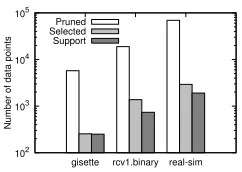
Pruned Selected Support
Figure 2: Effectiveness of the pruning
Efficiency
We evaluated the training time of each approach. Figure 1 shows the results with parameter ν values of 0.02, 0.04, and0.06. For the coherence criterion-based approach, we set thresholdµ0so that the number of support vectors isnν for
parameterν to ensure fair comparisons. Note thatν is the lower bound on the fraction of support vectors. Therefore, we changedνto evaluate our approach for various numbers of support vectors. For real-sim dataset, we omit the results of the active-set method-based approach and the shrinking approach since training could not be completed within a week. Figure 2 shows the number of data points included in set SandPof our approach and the number of support vectors after we have the optimal hyper-plane. In this figure, “Pruned”, “Selected”, and “Support” represent the number of selected data points in setS, pruned data points in setP, and support vectors, respectively, where we setν= 0.02.
10-4 10-3
10-2 10-1 100
gisette rcv1.binary real-sim
Objective function score
Quix Nystro..m Fourier
Coherence Active-set Shrinking
(1)ν= 0.02
10-4 10-3
10-2 10-1 100
gisette rcv1.binary real-sim
Objective function score
Quix Nystro..m Fourier
Coherence Active-set Shrinking
(2)ν= 0.04
10-4 10-3
10-2 10-1 100
gisette rcv1.binary real-sim
Objective function score
Quix Nystro..m Fourier
Coherence Active-set Shrinking
(3)ν= 0.06
Figure 3: Objective function score of each approach.
10-2 10-1 100
0.02 0.04 0.06
F-measure
Parameter ν
Quix Nystro..m Fourier
Coherence Active-set Shrinking
Figure 4: F-measures of output support vectors.
points. Since the coherence criterion-based approach can ef-ficiently check the data points by using the criterion, it is faster than the active-set method-based approach. However, the effectiveness of the coherence criterion-based approach is moderate. This is because, although it incrementally up-dates the Lagrange multipliers by using the Woodbury ma-trix identity, it needs to update the Lagrange multipliers ev-ery time data points are added to the set of support vectors. Although the shrinking approach can reduce data points be-fore applying the solver, it needs to compute parameterzi of each data point from the kernel functions in checking the optimality of the hyper-plane. Therefore, the shrinking approach does not effectively reduce the computation cost. On the other hand, our approach efficiently computes the upper and lower bounds of each data point before apply-ing the solver. In addition, we can effectively reduce sets of selected data points applied to the solver as shown in Fig-ure 2. Note that the number of applications of the solver in our approach,t, was at most two in the experiments. Even though we use the set of pruned data points in checking the optimality, we can efficiently check the optimality by using upper and lower bounds. Note that our approach is more ef-ficient than the incremental SVM approach (Laskov et al. 2006). Incremental SVM needs to iteratively add data point one by one. Therefore, it needsO(n|S|2) time to perform batch learning (n |S|) if SMO is used as the solver. On the other hand, we compute hyper-plane forsdata points and thus needsO(|S|2)time. Therefore, our approach is more
ef-ficient than the previous approaches.
Optimality
One major advantage of our approach is that it yields the optimal hyper-plane that minimizes the objective function
0 0.2 0.4 0.6 0.8 1
0.02 0.04 0.06
Training accuracy
Parameter ν
Quix Nystro..m.. Fourier
Coherence Active-set Shrinking
Figure 5: Training accuracy of each approach
100 101 102
103 104
gisette rcv1.binary real-sim
Wall clock time [s]
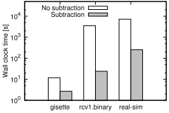
No subtraction Subtraction
Figure 6: Training time of the subtraction approach
given by Equation (1). In Figure 3, we show the scores of the objective function yielded by each approach for pa-rameterν values of 0.02,0.04, and0.06. In addition, Fig-ure 4 shows the F-measFig-ure against the original approach of one-class SVM in identifying support vectors, and Figure 5 show the training accuracy of each approach where we used gisette dataset. F-measure of an approach is1if the obtained support vectors by the approach exactly match those of the original approach.
heuristics have no theoretical foundation. Note that ap-proximate approaches result in reducing accuracy of SVM as demonstrated in the previous papers (Li et al. 2016; Yang et al. 2012). On the other hand, although our approach also discards data points it is carefully designed so that sup-port vectors of the optimal hyper-plane can be obtained. Therefore, as shown in Figure 4, our approach can accu-rately identify the support vectors for the given data points. As a result, the training accuracy of the proposed approach is high as shown in 5. Note that, as described in the preliminar-ies section, the training accuracy of one-class SVM cannot smaller than1−ν. Although the shrinking approach can ob-tained the optimal hyper-plane, it needs high computation cost as shown in Figure 1.
Subtraction approach
The proposed approach uses sparse vectorxˆi to efficiently compute the upper and lower bounds. So as to evaluate the effectiveness of this approach, we perform experiments. In Figure 6, we show the training times where we setν = 0.02. In this figure, “No subtraction” and “Subtraction” represent the results of approaches without and with the subtraction approaches, respectively. Note that gisette dataset obtained from the website of LIBSVM has numerical features.
Figure 6 shows that we can increase the training speed by reducing the number of non-zero elements. In order to increase the number of non-zero elements, the proposed ap-proach subtracts the most frequent value in each vector. As a result, our approach can use the sparse vectors in computing the bounds. Since we can effectively reduce non-zero ele-ments, we can increase the training efficiency of one-class SVM; the training time is up to147times faster by exploit-ing the subtraction approach.
Conclusions
In this paper, we proposed Quix, an efficient algorithm for one-class SVM that is guaranteed to yield the optimal hyper-plane. The proposed approach computes upper and lower bounds of a parameter that determines the hyper-plane to improve calculation efficiency. Experiments indicated that the proposed approach outperforms previous approaches in terms of efficiency and optimality. The proposed approach is an attractive option in the application of one-class SVM.
References
Cauwenberghs, G., and Poggio, T. A. 2000. Incremental and
Decremental Support Vector Machine Learning. InNIPS, 409–
415.
C¸ eker, H., and Upadhyaya, S. J. 2016. User Authentication with
Keystroke Dynamics in Long-text Data. InBTAS, 1–6.
Cristianini, N., and Shawe-Taylor, J. 2000.An Introduction to
Sup-port Vector Machines and Other Kernel-based Learning Methods. Cambridge University Press.
Drineas, P., and Mahoney, M. W. 2005. On the Nystr¨om Method for Approximating a Gram Matrix for Improved Kernel-based Learn-ing.Journal of Machine Learning Research6:2153–2175. Fisher, W.; Camp, T.; and Krzhizhanovskaya, V. V. 2016. Crack Detection in Earth Dam and Levee Passive Seismic Data Using
Support Vector Machines. InICCS, 577–586.
Fujiwara, Y.; Nakatsuji, M.; Shiokawa, H.; Mishima, T.; and Onizuka, M. 2013. Fast and Exact Top-k Algorithm for PageR-ank. InAAAI.
Fujiwara, Y.; Nakatsuji, M.; Shiokawa, H.; Ida, Y.; and Toyoda, M. 2015. Adaptive Message Update for Fast Aaffinity Propagation. In
SIGKDD, 309–318.
Fujiwara, Y.; Marumo, N.; Blondel, M.; Takeuchi, K.; Kim, H.; Iwata, T.; and Ueda, N. 2017a. Scaling Locally Linear Embedding. InSIGMOD, 1479–1492.
Fujiwara, Y.; Marumo, N.; Blondel, M.; Takeuchi, K.; Kim, H.; Iwata, T.; and Ueda, N. 2017b. SVD-based Screening for the
Graphical Lasso. InIJCAI, 1682–1688.
Gao, K. 2015. Online One-class SVMs with Active-set
Optimiza-tion for Data Streams. InICMLA, 116–121.
G´omez-Verdejo, V.; Arenas-Garc´ıa, J.; L´azaro-Gredilla, M.; and
Navia-V´azquez, ´A. 2011. Adaptive One-class Support Vector
Ma-chine. IEEE Trans. Signal Processing59(6):2975–2981.
Joachims, T. 1999. Advances in kernel methods. Cambridge, MA, USA: MIT Press. chapter Making Large-scale Support Vector Machine Learning Practical, 169–184.
Laskov, P.; Gehl, C.; Kr¨uger, S.; and M¨uller, K. 2006. Incremental Support Vector Learning: Analysis, Implementation and
Applica-tions.Journal of Machine Learning Research7:1909–1936.
Li, Z.; Yang, T.; Zhang, L.; and Jin, R. 2016. Fast and Accurate
Refined Nystr¨om-based Kernel SVM. InAAAI, 1830–1836.
Mishima, T., and Fujiwara, Y. 2015. Madeus: Database Live Mi-gration Middleware under Heavy Workloads for Cloud
Environ-ment. InSIGMOD, 315–329.
Musco, C., and Musco, C. 2017. Recursive Sampling for the
Nys-trom Method. InNIPS, 3836–3848.
Nakatsuji, M., and Fujiwara, Y. 2014. Linked Taxonomies to Cap-ture Users’ Subjective Assessments of Items to Facilitate Accurate Collaborative Filtering.Artif. Intell.207:52–68.
Nakatsuji, M.; Fujiwara, Y.; Toda, H.; Sawada, H.; Zheng, J.; and Hendler, J. A. 2014. Semantic Data Representation for Improving
Tensor Factorization. InAAAI, 2004–2012.
Noumir, Z.; Honeine, P.; and Richard, C. 2012. Online One-class
Machines Based on the Coherence Criterion. InEUSIPCO, 664–
668.
Platt, J. 1998. Sequential Minimal Optimization: A Fast Algorithm for Training Support Vector Machines. Technical report.
Rahimi, A., and Recht, B. 2007. Random Reatures for Large-scale
Kernel Machines. InNIPS, 1177–1184.
Sch¨olkopf, B.; Platt, J. C.; Shawe-Taylor, J.; Smola, A. J.; and
Williamson, R. C. 2001. Estimating the Support of a
High-dimensional Distribution.Neural Computation13(7):1443–1471.
Steele, J. M. 2004. The Cauchy-Schwarz Master Class: An
Intro-duction to the Art of Mathematical Inequalities. Cambridge Uni-versity Press.
Tanaka, Y.; Kurashima, T.; Fujiwara, Y.; Iwata, T.; and Sawada, H. 2016. Inferring Latent Triggers of Purchases with Consideration of
Social Effects and Media Advertisements. InWSDM, 543–552.
Wu, L.; Yen, I. E.; Chen, J.; and Yan, R. 2016. Revisiting Random Binning Features: Fast Convergence and Strong parallelizability.P
InKDD, 1265–1274.
Yang, T.; Li, Y.; Mahdavi, M.; Jin, R.; and Zhou, Z. 2012. Nystr¨om Method vs Random Fourier Features: A Theoretical and Empirical