The Thirty-Third AAAI Conference on Artificial Intelligence (AAAI-19)
Symmetry-Breaking Constraints for Grid-Based Multi-Agent Path Finding
∗Jiaoyang Li,
1Daniel Harabor,
2Peter J. Stuckey,
2Hang Ma,
1Sven Koenig
1 1University of Southern California2Monash University
[email protected],{daniel.harabor,peter.stuckey}@monash.edu,{hangma,skoenig}@usc.edu
Abstract
We describe a new way of reasoning about symmetric colli-sions for Multi-Agent Path Finding (MAPF) on 4-neighbor grids. We also introduce a symmetry-breaking constraint to resolve these conflicts. This specialized technique allows us to identify and eliminate, in a single step, all permutations of two currently assigned but incompatible paths. Each such per-mutation has exactly the same cost as a current path, and each one results in a new collision between the same two agents. We show that the addition of symmetry-breaking techniques can lead to an exponential reduction in the size of the search space of CBS, a popular framework for MAPF, and report significant improvements in both runtime and success rate versus CBSH and EPEA* – two recent and state-of-the-art MAPF algorithms.
1
Introduction
Multi-Agent Path Finding (MAPF) is the planning problem of finding a set of paths for a team of agents. Each agent is required to move from an initial start location to a specified goal location, while avoiding conflicts with other agents. A conflict (i.e., collision) happens when two agents stay at the same vertex or traverse the same edge at the same time. Such problems appear in a range of application areas, includ-ing warehouse logistics (Wurman, D’Andrea, and Mountz 2008), office robots (Veloso et al. 2015), aircraft-towing ve-hicles (Morris et al. 2016) and computer games (Silver 2005; Ma et al. 2017).
MAPF is known to be NP-hard on general graphs (Yu and LaValle 2013b; Ma et al. 2016b), planar graphs (Yu 2016) and grids (Banfi, Basilico, and Amigoni 2017). De-spite these intractability results and due to the substantial in-terest in applications, numerous optimal MAPF algorithms have been proposed in recent years. Approaches include re-ducing MAPF to instances of other well known problems
∗
The research at the University of Southern California was sup-ported by the National Science Foundation (NSF) under grant num-bers 1409987, 1724392, 1817189 and 1837779 as well as a gift from Amazon. The views and conclusions contained in this docu-ment are those of the authors and should not be interpreted as rep-resenting the official policies, either expressed or implied, of the sponsoring organizations, agencies or the U.S. government. Copyright c2019, Association for the Advancement of Artificial Intelligence (www.aaai.org). All rights reserved.
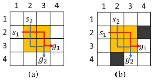
(a) (b)
Figure 1: Two situations involving symmetric conflicts be-tween two agents. (a) highlights the problem in general: ev-ery shortest path for one agent conflicts with evev-ery shortest path for the other agent somewhere in the yellow rectangular area. (b) shows a cardinal conflict, a related class of conflicts which requires that all shortest paths for each agent must pass through a common location at the same timestep: here location(3,3)at timestep3.
(e.g., multi-commodity flow (Yu and LaValle 2013a), sat-isfiability (Surynek et al. 2016) and Answer Set Program-ming (Erdem et al. 2013)); solving MAPF with a single inte-grated A*-search (Standley 2010; Wagner and Choset 2011; Goldenberg et al. 2014); and solving MAPF with a two-level search (Sharon et al. 2013; 2015; Boyarski et al. 2015; Felner et al. 2018), which constructs a plan by keeping track of constraints between agents at a high level and computing paths consistent with those constraints at a low level, one agent at a time. More detailed surveys are given in (Ma et al. 2016a; Felner et al. 2017).
con-flicts and non-cardinal rectangle concon-flicts. We also introduce
barrier constraintsthat are able to resolve these rectangle conflicts in a single step and demonstrate, in principle and in practice, that the addition of barrier constraints can achieve an exponential reduction in the number of nodes expanded by Conflict-Based Search (CBS), a popular state-of-the-art MAPF framework.
2
Preliminaries
A MAPF problem is defined by a graphG= (V, E)and a set ofmagents{a1, . . . , am}. Each agentaihas a start ver-texsi∈V and a goal vertexgi∈V. Time is discretized into timesteps. At each timestep, every agent can either move to an adjacent vertex or wait at its current vertex. Both move and wait actions have unit cost unless the agent terminally waits at its goal vertex, which has zero cost. We call the tuplehai, aj, v, tiavertex conflictiff agentsai andaj oc-cupy the same vertexv ∈ V at the same timestep t, and hai, aj, u, v, tianedge conflictiff agentsaiandajtraverse the same edge(u, v)∈Ein opposite directions at the same timestep t. Our task is to find a set of conflict-free paths which move all agents from their start vertices to their goal vertices while minimizing thesum of their individual path costs(SIC). In this paper, graphGis always a 4-neighbor grid whose vertices are unblocked cells and whose edges connect vertices corresponding to adjacent unblocked cells in the four main compass directions.
3
Conflict-Based Search
Conflict-Based Search(CBS) (Sharon et al. 2015) is a two-level search algorithm for MAPF. At the low two-level, CBS in-vokes a space-time A* search to find a shortest path for each agent that satisfies some spatio-temporal constraints added by the high level. It break ties by preferring the path that has the fewest conflicts with the paths of other agents. At the high level, CBS performs a best-first search on a binary con-straint tree(CT). Each CT node contains a set of paths, one for each agent, and also a set of spatio-temporal constraints that are used to coordinate agents and avoid conflicts. The cost of a CT node is the SIC of its current paths. CBS pro-ceeds from one CT node to the next, checking for conflicts and calling its low-level search to replan paths one at a time. CBS succeeds when the current CT node is conflict-free, which corresponds to an optimal solution.
Constraints:A constraint is a spatio-temporal restriction introduced by CBS to resolve situations where the paths of two agents are in conflict. Specifically, avertex constraint
hai, v, ti means that agent ai is prohibited from occupy-ing vertex v at timestep t. Similarly, an edge constraint
hai, u, v, timeans that agentai is prohibited from travers-ing edge(u, v)at timestept.
Splits:When CBS expands a CT nodeN, it checks for pairwise conflicts among the current paths. If there are none, thenN is a goal CT node and CBS terminates. Otherwise, CBS chooses one of the conflicts and resolves it by split-tingNinto two child CT nodes. In each child CT node, one agent from the conflict is forbidden to use the contested ver-tex or edge by way of an additional constraint. The path of
this agent becomes invalidated and must be replanned by a low-level search. All other paths remain unchanged. With two child CT nodes per conflict, CBS guarantees optimality, exploring both ways of resolving each conflict.
Cardinal, semi-cardinal and non-cardinal conflicts:
Boyarski et al. (2015) categorize conflicts into three differ-ent types, and they show that prioritizing among conflicts improves performance. The highest priority is given to car-dinal conflicts, which they define as follows:
[A conflict]C=hai, aj, v, tiis cardinal if all the con-sistent optimal paths for both [agents]aiandajinclude vertexvat timestept.
An example of such a conflict is shown in Figure 1(b). Every possible way of resolving the cardinal conflict ha1, a2,(3,3),3irequires one of the agents to wait for the
other or take a detour. That means, when CBS splits on a car-dinal conflict, it produces two child CT nodes whose costs are both strictly higher than the current CT node. In this work, we show that there exist other types of conflicts which have the same result when splitting on them but which can-not be detected using the present definition, such as shown in the example in Figure 1(a). We therefore introduce a revised and more general definition:
Definition 1. A conflict C iscardinaliff replanning for any agent involved in the conflict increases the SIC.
Once all cardinal conflicts are processed, the next highest priority is given tosemi-cardinal conflicts, which Boyarski et al. (2015) define as:
[A conflict]C=hai, aj, v, tiis semi-cardinal if all the consistent optimal paths of one agent include vertexv
at timestep t, but the other agent has such a path that does not includevat timestept.
Similarly, we give a revised and more general definition:
Definition 2. A conflict C issemi-cardinaliff replanning for one agent involved in the conflict always increases the SIC while replanning for the other agent does not.
Any conflict which is not cardinal or semi-cardinal is said to be non-cardinal. These can be processed in any order after the other conflicts, though a popular strategy involves choosing the earliest non-cardinal conflict first.
Admissible heuristics: The high-level of CBS consists of a best-first search that prioritizes for expansion CT nodes with the smallest SIC. Felner et al. (2018) show that the effi-ciency of the high-level search can be improved through the addition of admissible heuristics. The suggested algorithm, CBSH, proceeds by building a conflict graph, whose ver-tices represent agents and edges represent cardinal conflicts of the current paths. It can be shown that the value of the minimum vertex cover of the conflict graph is an admissible and consistent lower bound on the cost-to-go. The addition of heuristics to the high-level search often produces smaller CTs and decreases the runtime of CBS by a large factor.
Figure 2: The CT of CBS and CBSH (without the 2 blue CT nodes for CBSH) when resolving a 1×3 cardinal rectangle conflict.
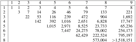
Table 1: Number of CT nodes expanded by CBSH on MAPF instances where 2 agents are involved in one cardinal rect-angle conflict. The first column and first row are the width and length of the rectangular area.
1 2 3 4 5 6 7 8 9
1 1 1 2 3 4 5 6 7 8
2 3 7 14 26 46 79 133 221
3 22 53 116 239 472 904 1,692
4 142 392 1,016 2,651 6,828 17,747
5 1,015 2,971 8,525 23,733 65,236
6 7,447 24,275 78,002 254,173
7 62,429 222,524 795,197
8 573,004 >1,518,151
of CT nodes resulting from it.
Figure 2 illustrates the issue. All shortest paths of agents
a1anda2cross the 1×3 yellow rectangular area.a1 has 1
shortest path with cost 4 whilea2has 6 shortest paths with
cost 4. Thus, the cost of the root CT node of CBS is 8. How-ever, each of the 6 combinations of these paths has a vertex conflict in one of the yellow cells. Consequently, this is a cardinal rectangle conflict, and the optimal solution cost is 9. The CT of CBS consists of 3 non-goal CT nodes with cost 8 and 4 goal CT nodes with cost 9. The CT of CBSH only saves the last 2 goal CT nodes (in blue).
When the rectangular area is larger, CBS performs worse. Sharon et al. (2015) show that, to resolve the 2×2 cardinal rectangle conflict in Figure 1(a), CBS generates 5 non-goal CT nodes and 6 goal CT nodes (and, CBSH generates 5 CT non-goal nodes and 2 CT goal nodes). To illustrate this is-sue further, we ran CBSH on MAPF instances where two agents are involved in a cardinal rectangle conflict of differ-ent sizes. Surprisingly, the number of expanded CT nodes, as shown in Table 1, is exponential in the length and width of the rectangular area. For a small 8×9 rectangular area, CBSH expands already more than 1 million CT nodes and fails to solve the MAPF instance within 5 minutes.
5
Cardinal Rectangle Reasoning for Entire
Paths
In this section, we present a simple algorithm for identifying cardinal rectangle conflicts and introduce a new type of con-straints, called barrier concon-straints, to resolve such conflicts efficiently. We refer to a nodeS as a three-element tuple (S.x, S.y, S.t)corresponding to an agent staying in location (S.x, S.y)at timestepS.t. We refer to avalid path(orpath
for short) of an agent as a path (sequences of nodes whose locations can repeat and whose timesteps are 0,1,2, . . .) from its start location to its goal location that satisfies its constraints in the CT node but ignores paths of other agents and anoptimal pathof an agent as its shortest valid path.
5.1
Identify Cardinal Rectangle Conflicts
Assume that two agents ai and aj have a vertex conflict hai, aj, v, ti. Let nodes Si, Sj, Gi and Gj be the corre-sponding start and goal nodes (Figure 3(a)). We define the
rectangular area (or rectangle for short) as the intersec-tion of theSi-Gi rectangle and theSj-Gj rectangle, where
Sk-Gk rectangle (k = i, j) represents the rectangle whose diagonal corners are in location (Sk.x, Sk.y) and location (Gk.x, Gk.y), respectively. The first two requirements for a cardinal rectangle conflict are intuitive: (1) both agents fol-low theirManhattan-optimalpaths, i.e., the cost of each path equals the Manhattan distance from its start node to its goal node, and (2) the distances from each location inside the rectangle to the locations of the two start nodes are equal, which can be simplified to the requirement that both agents move in the same direction in both dimensions (because we already know that the distances from locationvto the loca-tion of nodeSiand the location of nodeSjare equal):
|Si.x−Gi.x|+|Si.y−Gi.y|=Gi.t−Si.t >0 (1)
|Sj.x−Gj.x|+|Sj.y−Gj.y|=Gj.t−Sj.t >0 (2)
(Si.x−Gi.x)(Sj.x−Gj.x)≥0 (3)
(Si.y−Gi.y)(Sj.y−Gj.y)≥0. (4)
However, these two requirements do not guarantee that all combinations of optimal paths conflict. Figures 3(b) and 3(c) are two counterexamples where at least one agent has a by-pass through which the agent can reach its goal node without entering the rectangle, and thus does not conflict with the other agent. The difference between these two conflicts and the cardinal rectangle conflict in Figure 3(a) is that their goal nodes are located differently compared to their start nodes. Therefore, the third requirement is that the start and goal nodes have opposite relative locations in both dimensions:
(Si.x−Sj.x)(Gi.x−Gj.x)≤0 (5)
(Si.y−Sj.y)(Gi.y−Gj.y)≤0. (6)
To sum up, if agentsaiandajhave a vertex conflict and their corresponding start and goal nodes satisfy Equations (1) to (6), then agentsaiandajare involved in a cardinal rect-angle conflict.
5.2
Calculate Corner Nodes of the Rectangle
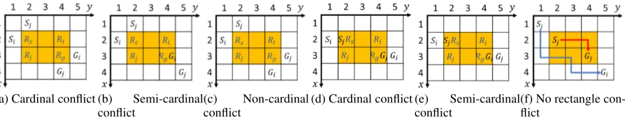
We refer to the four corner nodes of the rectangle asRs,Rg,(a) Cardinal conflict (b) Semi-cardinal conflict
(c) Non-cardinal conflict
(d) Cardinal conflict (e) Semi-cardinal conflict
(f) No rectangle con-flict
Figure 3: Some examples of rectangle conflicts. The locations of the start and goal nodes are shown in the figures.Gk.t =
Sk.t+|Gk.x−Sk.x|+|Gk.y−Sk.y|, k =i, j. In (a), (b) and (c),Si.t=Sj.t; in (d) and (e),Si.t=Sj.t−1; and, in (e),
Si.t=Sj.t−2.
Sj, respectively (Figure 3(a)). The timestep of each node is defined as the timestep when an optimal path of agent
ai or aj reaches the location of the node. We analyze all combinations of relative locations of start and goal nodes and come up with the following way to calculate them: For the locations ofRsandRg:
Rs.x=
Si.x, Si.x=Gi.x
max{Si.x, Sj.x}, Si.x < Gi.x
min{Si.x, Sj.x}, Si.x > Gi.x
(7)
Rg.x=
Gi.x, Si.x=Gi.x
min{Gi.x, Gj.x}, Si.x < Gi.x
max{Gi.x, Gj.x}, Si.x > Gi.x.
(8)
We can calculateRs.yandRg.yby replacing allxbyyin Equations (7) and (8). Next, for the locations ofRiandRj, if (Si.x−Sj.x)(Sj.x−Rg.x)≥0, thenRi.x=Rg.x,Ri.y=
Si.y,Rj.x = Sj.xandRj.y = Rg.y; else,Ri.x = Si.x,
Ri.y =Rg.y,Rj.x=Rg.xandRj.y =Sj.y. Finally, for the timesteps of all corner nodesRk(k=i, j, s, g),Rk.t=
Si.t+|Si.x−Rk.x|+|Si.y−Rk.y|.
5.3
Add Barrier Constraints
Since all combinations of the optimal paths of the agents conflict, we resolve the cardinal rectangle conflict by giv-ing one agent priority within the rectangle and forcgiv-ing the other agent to leave it later or take a detour. To integrate this idea into CBS, we introduce the barrier constraint,
B(ak, Rk, Rg) (k = i, j), which is a set of vertex con-straints that prohibits agent ak from occupying all loca-tions along the border of the rectangle that is opposite of its start node (i.e., from Rk to Rg) at the timestep when
ak would optimally reach the location. For example, in Figure 3(a), two barrier constraints are B(ai, Ri, Rg) = {hai,(2 +n,4),3 +ni|n = 0,1} and B(aj, Rj, Rg) = {haj,(3,2 +n),2 +ni|n= 0,1,2}.B(ak, Rk, Rg)blocks all possible paths for ak that reach its goal node Gk via the rectangle, and thus forcesak to wait or take a detour. When resolving a cardinal rectangle conflict, we generate two child CT nodes and addB(ai, Ri, Rg)to one of them andB(aj, Rj, Rg)to the other one. We now present two ob-vious properties of barrier constraints.
Property 1. For all combinations of paths of agentsaiand
aj with a cardinal rectangle conflict, if one path violates
B(ai, Ri, Rg) and the other path violates B(aj, Rj, Rg),
then the two paths have one or more vertex conflicts within the rectangle.
Proof. We assume that the vertex conflict between agents
ai and aj that underlies the cardinal rectangle conflict is hai, aj,(C.x, C.y), C.ti. We then assumeSi.x ≤ C.xand
Si.y ≤ C.y without loss of generality (because the prob-lem is invariant under rotations of axes). According to Equa-tions (1) to (4),
max{Si.x, Sj.x} ≤C.x≤min{Gi.x, Gj.x} (9)
max{Si.y, Sj.y} ≤C.y≤min{Gi.y, Gj.y} (10)
(C.x−Si.x) + (C.y−Si.y) = (C.x−Sj.x) + (C.y−Sj.y).
(11)
From Equation (11), we know
Si.x+Si.y=Sj.x+Sj.y. (12)
We can assume thatSi.x≥Sj.xwithout loss of generality (because the problem is invariant under swaps of the indexes of agents), which impliesSi.y ≤Sj.y. From Equations (9) and (10) and the method for calculating rectangle corner nodes in Section 5.2, we haveRg.x= min{Gi.x, Gj.x} ≥
Si.x, Rg.y = min{Gi.y, Gj.y} ≥ Sj.y, Ri.x = Si.x,
Ri.y=Rg.y,Rj.x=Rg.xandRj.y=Sj.y. Thus,
Sj.x≤Si.x=Ri.x≤Rg.x=Rj.x (13)
Si.y≤Sj.y=Rj.y≤Rg.y=Ri.y. (14)
Consequently, the relative locations of the start, goal and rectangle corner nodes are exactly the same as given in Figure 3(a). For every node Ni on the borderRi-Rg (i.e.,
Ri.x≤Ni.x≤Rg.x, Ni.y =Rg.y,Ni.t=Ri.t+Ni.x−
Ri.x) and every nodeNjon the borderRj-Rg(i.e.,Nj.x=
Rg.x, Rj.y≤Nj.y ≤Rg.y,Nj.t=Rj.t+Nj.y−Rj.y), we need to prove that the path fromSitoNi and the path from Sj toNj have at least one node in common within the rectangle. Since Sj.x ≤ Si.x ≤ Ni.x ≤ Nj.xand
Si.y ≤Sj.y ≤Nj.y ≤Ni.y, theSi-Nirectangle and the
Sj-Njrectangle consist of a cross shape, which implies that the path fromSi toNiand the path fromSj toNj have at least one location in common within the intersection of the
Si-Nirectangle and theSj-Njrectangle, i.e., this location is within the rectangle. By the definition of rectangle conflicts, the two paths traverse this location at the same timestep, i.e., they have at least one node in common within the rectan-gle.
Property 2. If agentsai andaj have a cardinal rectangle
conflict, then the cost of any path of agentak(k=i, j) that
satisfiesB(ak, Rk, Rg)is larger than the cost of an optimal
Proof. We use the same assumptions as in the proof for Property 1. Then, Equations (13) and (14) also hold here. According to Equation (5), Si.x = Ri.x ≤ Rg.x =
Gi.x. Any optimal path that connects locations(Si.x, Si.y) and (Gi.x, Gi.y) has at least one of the nodes {(Ri.x+
n, Ri.y, Ri.t+n)|n= 0, . . . , Rg.x−Ri.x}. But all of these nodes are constrained byB(ai, Ri, Rg). Therefore, the cost of any path of agentaithat satisfiesB(ai, Ri, Rg)is larger than the cost of an optimal path of agentai. The proof for
k=jcan be derived analogously using Equation (6) instead of Equation (5).
Property 1 is important because CBS requires the con-straints added to child CT nodes to not block any conflict-free paths, which is why we add constraints that force an agent to leave the rectangle later rather than enter the it later.
5.4
CBSH-CR
We now present our first algorithm, CBSH with cardinal rectangle reasoning(CBSH-CR). It is identical to CBSH ex-cept for the following four modifications.
Perform splits: When the chosen conflict is a cardi-nal rectangle conflict, CBSH-CR addsB(ai, Ri, Rg)to one child CT node andB(aj, Rj, Rg)to the other child CT node. Then, in both child CT nodes, the rectangle conflict is re-solved by one of the agents increasing its cost.
Classify conflicts:CBSH-CR first classifies vertex/edge conflicts into cardinal, semi-cardinal and non-cardinal con-flicts. It then finds cardinal rectangle conflicts among all semi- and non-cardinal vertex conflicts.
Prioritize conflicts: It follows from Definition 1 and Properties 1 and 2 that both cardinal rectangle conflicts and cardinal vertex/edge conflicts are cardinal conflicts. There-fore, CBSH-CR chooses cardinal conflicts first, then semi-cardinal conflicts and last non-semi-cardinal conflicts. It breaks ties by preferring the earliest conflict, where we defineRs.t as the timestep of a cardinal rectangle conflict.
Calculate heuristics:It uses all cardinal conflicts (includ-ing cardinal rectangle conflicts) to compute the heuristics for the high-level search.
Now we show that CBSH-CR is complete and optimal.
Lemma 1. For every costc, there is a finite number of CT nodes with costc.
Proof. The number of conflicts withinctimesteps is finite, and, once a conflict is chosen at a CT nodeN, it never ap-pears again in the subtree of N. Therefore, the number of CT nodes is also finite.
Theorem 2. CBSH-CR is complete and optimal.
Proof. The proof is similar to the proof for the optimality and completeness of CBS (Sharon et al. 2015). The low-level search always returns an optimal path, the high-low-level search always chooses a CT node with minimum f-value to expand, and the expansion does not lose any conflict-free paths (Property 1). Therefore, the first chosen CT node whose paths are conflict-free has a set of conflict-free paths with minimum SIC (i.e., CBSH-CR is optimal). Besides, the
f-value of CT nodes are non-decreasing in expansion order.
It follows from Lemma 1 that, if there exist solutions, a so-lution must be found after expanding a finite number of CT nodes whose costs are no more than the optimal cost (i.e., CBSH-CR is complete).
6
Rectangle Reasoning for Entire Paths
Reasoning about cardinal rectangle conflicts does not elimi-nate all symmetric conflicts on grids for CBS. For instance, the conflict in Figure 3(b) is not a cardinal rectangle conflict because agentaj has an optimal bypass outside of the rect-angle. However, if location(2,5)at timestep4and location (3,5)at timestep5are occupied by other agents, whenever the low-level search of CBS replans agent aj’s path, it al-ways returns a path that conflicts with agent ai’s path, be-cause the low-level search uses the number of conflicts with other agents as the tie-breaking rule. Therefore, CBS again generates many CT nodes before finally finding conflict-free paths. We refer to such cases assemi-cardinal rectangle con-flicts. Similarly, we refer to cases with symmetric conflicts where both agents have bypasses asnon-cardinal rectangle conflicts, like the case in Figure 3(c). Together with cardinal rectangle conflicts, we refer to these three types of conflicts asrectangle conflicts.We now show how to identify and classify rectangle con-flicts. If agentsaiandajhave a vertex conflict, then they are involved in a rectangle conflict iff their start and goal nodes satisfy Equations (1) to (4). Moreover, if they also satisfy Equations (5) and (6), it is cardinal; if they also satisfy only one of these equations, it is semi-cardinal; and if they sat-isfy neither equation, it is non-cardinal. Property 1 holds for all types of rectangle conflicts. It follows from the proof for Property 2 that, when resolving a semi-cardinal rectangle conflict by barrier constraints, at least one of the child CT nodes has to increase its SIC. But for a non-cardinal rectan-gle conflict, both child CT nodes may not change their SICs.
6.1
CBSH-R
We now introduce the second algorithm,CBSH with rectan-gle reasoning(CBSH-R). It is identical to CBSH-CR except for the following three modifications.
Perform splits: CBSH-R uses barrier constraints to re-solve all rectangle conflicts (not only cardinal ones).
Classify conflicts:After classifying all vertex/edge con-flicts, CBSH-R checks all semi- and non-cardinal vertex conflicts to identify and classify rectangle conflicts. If a semi-/non-cardinal rectangle conflict has been resolved in one of the ancestors of the current CT node, it ignores this rectangle conflict, otherwise it could always choose to re-solve the same rectangle conflict and thus be in a cycle for-ever. A semi-/non-cardinal rectangle conflict can be found multiple times in a CT branch because its barrier constraint does not disallow all optimal paths that traverse locations in-side the rectangle. For example, in Figure 3(c), both agents
ai andaj have optimal paths that contains nodeRsbut do not contain nodes that are constrained byB(ai, Ri, Rg)and
(a) (b)
Figure 4: Rectangle conflicts between path segments. In Fig-ure (b),a2follows the red solid arrow but waits at(1,4)or
(2,4)for one timestep because of constraints.
Prioritize conflicts:CBSH-R uses the same conflict pri-oritization as CBSH-CR, except that it adds a tie-breaking rule for semi-/non-cardinal rectangle conflicts. Since our reasoning method ignores obstacles and constraints inside the rectangle, it is possible that both child CT nodes increase their costs when CBSH-R resolves a semi-/non-cardinal rectangle conflict using barrier constraints. Therefore, for all semi-cardinal conflicts, it prefers semi-cardinal rectangle conflicts to semi-cardinal vertex/edge conflicts. Similarly, for all non-cardinal conflicts, it prefers non-cardinal rectan-gle conflicts to non-cardinal vertex/edge conflicts. The sec-ondary tie-breaking rule is still to prefer the earliest conflict, where we defineRs.tas the timestep of a rectangle conflict.
Theorem 3. CBSH-R is complete and optimal.
Proof. Since all chosen rectangle conflicts are different in any CT branch, Lemma 1 still holds. Property 1 also holds for semi-/non-cardinal rectangle conflicts. Therefore, we can directly use the proof for Theorem 2 without changes.
7
Rectangle Reasoning for Path Segments
Our rectangle reasoning methods so far ignore obstacles and constraints, so they can reason only about the rectangle flicts for entire paths. In some cases, however, rectangle con-flicts exist for path segments but not entire paths, such as the cardinal rectangle conflict in Figure 4(a). Since the paths are not Manhattan-optimal, our rectangle reasoning methods so far fail to identify the rectangle conflict. Therefore, in this section, we discuss a rectangle reasoning method for path segments using MDDs.7.1
Identify Rectangle Conflicts using MDDs
A Multi-Valued Decision Diagram (MDD) (Sharon et al. 2013)M DDi for agentai is a directed acyclic graph that consists of all optimal paths of agentai. The nodes at depthtinM DDicorrespond to all possible locations at timestep
t in these paths. If M DDi has only one node(x, y, t) at deptht, we call this node asingleton, and all optimal paths of agentaitraverse location(x, y)at timestept. CBSH uses singletons in MDDs to classify cardinal, semi-cardinal and non-cardinal vertex/edge conflicts.
MDDs offer information about the impact of obstacles in the grid and constraints imposed on an agent, and thus help us to reason about its path segments. We extend rectan-gle reasoning to reasoning about rectanrectan-gle conflicts between two path segments, each of which starts at a singleton (called
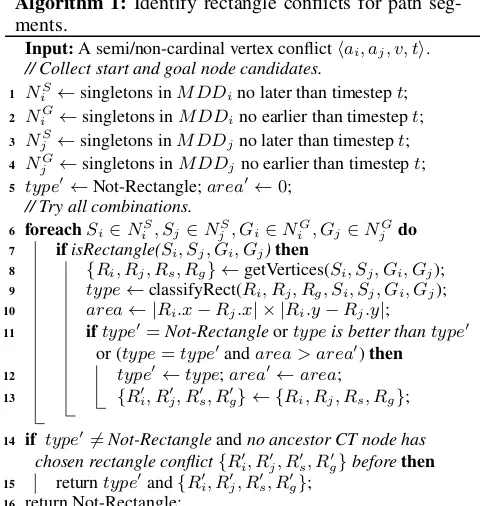
Algorithm 1:Identify rectangle conflicts for path seg-ments.
Input:A semi/non-cardinal vertex conflicthai, aj, v, ti.
// Collect start and goal node candidates.
1 NiS←singletons inM DDino later than timestept;
2 NiG←singletons inM DDino earlier than timestept;
3 NjS←singletons inM DDjno later than timestept;
4 NjG←singletons inM DDjno earlier than timestept;
5 type0←Not-Rectangle;area0←0; // Try all combinations.
6 foreachSi∈NiS, Sj∈NjS, Gi∈NiG, Gj∈NjGdo
7 ifisRectangle(Si, Sj, Gi, Gj)then
8 {Ri, Rj, Rs, Rg} ←getVertices(Si, Sj, Gi, Gj);
9 type←classifyRect(Ri, Rj, Rg, Si, Sj, Gi, Gj);
10 area← |Ri.x−Rj.x| × |Ri.y−Rj.y|;
11 iftype0=Not-Rectangleortypeis better thantype0
or (type=type0andarea > area0)then
12 type0←type;area0←area;
13 {R0i, R0j, Rs0, R0g} ← {Ri, Rj, Rs, Rg};
14 if type06=Not-Rectangleandno ancestor CT node has chosen rectangle conflict{R0i, R
0
j, R
0
s, R
0
g}beforethen
15 returntype0and{R0i, R
0
j, R
0
s, R
0
g};
16 return Not-Rectangle;
its start node) and ends at another singleton (called its goal node). If we find a rectangle conflict for a combination of start and goal nodes, we can impose barrier constraints.
Algorithm 1 shows the pseudo-code. It first treats all sin-gletons as start and goal node candidates (Lines 1-4) and then tries all combinations to find rectangle conflicts. If mul-tiple rectangle conflicts are identified, it prefers one of the highest priority type and breaks ties by preferring a con-flict with the largest rectangle area (Line 11). Line 14 pro-hibits choosing the same rectangle conflict more than once in any CT branch. We discuss details of the three functions on Lines 7, 8 and 9 in Section 7.3.
7.2
Add Modified Barrier Constraints
When reasoning about entire paths, all paths of agentai al-ways traverse its start nodeSi. However, path segments do not necessarily traverse its start nodeSi. In this case, barrier constraints may disallow pairs of conflict-free paths and thus lose the completeness and optimality guarantees.
Figure 4(b) provides a counterexample where a CT node
N has the set of constraints listed in the figure. The con-straints force agenta2to wait for at least one timestep before
reaching its goal location. It can either wait before entering the rectangle, which leads to a conflict with agenta1, or
en-ter the rectangle without waiting and wait laen-ter, which might avoid conflicts with agent a1. However, all optimal paths
of agenta2 inN (whose costs are 6) have to wait for one
timestep before entering the rectangle (seeM DD2 shown
in the figure). Therefore, node S2 = (2,4,2)is a
single-ton, and agentsa1anda2have a cardinal rectangle conflict.
agent a1 directly follows the blue arrow (which traverses
node(3,5,4) constrained byB(a1, R1, Rg)) and agenta2
follows the dotted red arrow but waits at location (4,4) for 2timesteps (which traverses node (4,4,4) constrained byB(a2, R2, Rg)). Barrier constraints fail here because the constrained node(4,4,4)is not inM DD2 and thus agent
a2could have a path with a larger cost that does not traverse
nodeS2but traverses node(4,4,4).
Therefore, we add a barrier constraint only for nodes that are in the current MDD of the agent. We call this a modi-fied barrier constraintB0(ak, Rk, Rg) = {hak,(x, y), ti ∈
B(ak, Rk, Rg)|(x, y, t)∈M DDk}(k=i, j), and its prop-erties are discussed in Section 7.3.
7.3
CBSH-RM
Our last algorithm is CBSH with rectangle reasoning by MDDs (CBSH-RM), which reasons about rectangle con-flicts between path segments. It uses Algorithm 1 to iden-tify and classify rectangle conflicts and uses modified barrier constraints to resolve them.
Previously, all start nodes were at timestep0, and thus their distances to the rectangle were equal. However, now we allow start nodes to be at different timesteps, e.g.,S1=
(5,2,1) and S2 = (5,3,2) in Figure 4(a). We thus need
to modify how to identify rectangle conflicts, calculate rect-angle corner nodes and classify rectrect-angle conflicts, corre-sponding to the three functions on Lines 7, 8 and 9 of Algo-rithm 1, respectively.
Identify rectangle conflicts:The start and goal nodes of a rectangle conflict have to satisfy not only Equations (1) to (4) but also
(Si.x−Sj.x)(Si.y−Sj.y)(Si.x−Gi.x)(Si.y−Gi.y)≤0.
(15)
This guarantees that the start nodes are on different borders of the rectangle since, otherwise, adding modified barrier constraints might lose a pair of paths that allow both agents to reach the constrained border without waiting, such as in the example of Figure 3(f). We also require thatSi 6= Sj, otherwise the two agents have a cardinal vertex conflict at nodeSiand CBS constraints can resolve it in a single step.
Calculate rectangle corner nodes:The method in Sec-tion 5.2 can miscalculateRi andRj when Si.x = Sj.x, such as in Figures 3(d) and 3(e). Instead, we calculateRi and Rj with the following method when Si.x = Sj.x: If (Si.y −Sj.y)(Sj.y −Rg) ≤ 0, then Ri.x = Rg.x,
Ri.y = Si.y,Rj.x = Sj.xandRj.y = Rg.y; otherwise,
Ri.x=Si.x,Ri.y=Rg.y,Rj.x=Rg.xandRj.y=Sj.y.
Classify rectangle conflicts: Similarly, Equations (5) and (6) misclassify rectangle conflicts when Si.x = Sj.x orSi.y =Sj.y. Instead, we classify rectangle conflicts us-ing the corner nodes of their rectangles. Since we always add modified barrier constraints along two adjacent borders of the rectangle, we only need to compare the length and width of the rectangle with those of theSi-Gi andSj-Gj rectangles. Consider the two equations:
Rk.x−Rg.x=Sk.x−Gk.x (16)
Rk.y−Rg.y=Sk.y−Gk.y. (17)
If one holds fork = iand the other one holds fork = j, the rectangle conflict is cardinal; if only one of them holds fork=iork=j, it is semi-cardinal; otherwise, it is non-cardinal.
Lemma 4. If agentsaiandajhave a rectangle conflict, any
path of agentak(k=i, j) that traverses a node constrained
byB0(ak, Rk, Rg)also traverses its start nodeSk.
Proof. Let Nk be a node constrained by B0(ak, Rk, Rg). Thus nodeNkis inM DDk. Then, any node before timestep
Nk.ton any path of agentakthat traverses nodeNk is also in M DDk. Since node Sk is a singleton of M DDk, any path of agent ak that traverses node Nk also traverses its start nodeSk.
Property 3. For all combinations of paths of agents ai
and aj with a rectangle conflict, if one path violates
B0(ai, Ri, Rg)and the other path violatesB0(aj, Rj, Rg),
then the two paths have one or more vertex conflicts within the rectangle.
Proof. By Lemma 4, we need to prove that any path of agent
ai from its start node Si to one of the nodes constrained by B0(ai, Ri, Rg)and any path of agent aj from its start nodeSjto one of the nodes constrained byB0(aj, Rj, Rg) have at least one node in common within the rectangle. This holds by applying the proof for Property 1 after replacing Equations (11) and (12) by Equation (15) and replacing the method for calculating rectangle corner nodes in Section 5.2 by the method in this section.
Property 4. If agents ai and aj have a rectangle conflict
and one of the Equations(16)and(17)holds fork(k=i, j), the cost of any path of agentakthat satisfiesB0(ak, Rk, Rg)
is larger than the cost of an optimal path of agentak.
Proof. Since nodesSk andGk are singletons, all optimal paths contain these two nodes. If one of Equations (16) and (17) holds, any path from nodeSkto nodeGktraverses at least one node constrained byB0(ak, Rk, Rg). So, all op-timal paths violate B0(ak, Rk, Rg). Therefore, the cost of any path of agentak that satisfiesB0(ak, Rk, Rg)is larger than the cost of an optimal path of agentak.
Theorem 5. CBSH-RM is complete and optimal.
Proof. The proof for Theorem 3 applies after replacing Properties 1 and 2 by Properties 3 and 4, respectively.
8
Experimental Results
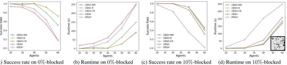
(a) Success rate on0%-blocked (b) Runtime on0%-blocked (c) Success rate on10%-blocked (d) Runtime on10%-blocked
Figure 5: Results on 20×20 grids with0%and10%blocked cells. (a) and (c) plot the success rates within 5 minutes. (b) and (d) plot the runtimes, where the runtime limit of 5 minutes is included in the average for unsolved instances. Many parts of the blue lines in (a) and (b) are hidden by the yellow lines.
(a) Success rate on den520d (b) Runtime on den520d (c) Success rate on lak503d (d) Runtime on lak503d
Figure 6: Results on the game grids den520d and lak503d. (a) and (c) plot the success rates within 5 minutes. (b) and (d) plot the runtimes, where the runtime limit of 5 minutes is included in the average for unsolved instances.
Table 2: Results on 20×20 grids. The first “Ins” column shows the number of instances solved by both CBSH and CBSH-RM, and the following columns show results on these instances. Similarly, the second “Ins” column shows the number of instances solved by CBSH-CR, CBSH-R and CBSH-RM, and the following columns show results on these instances.
m Ins CBSHRuntime (s)RM CBSHCT NodesRM Ins CRRuntime (s)R RM CR CT NodesR RM
0%
30 46 6.2 0.02 29,506 87 49 0.06 0.03 0.02 222 89 82
40 40 2.1 0.02 10,889 105 50 2.2 2.1 2.1 11,282 11,029 10,140
50 27 14.8 1.4 92,627 5,925 39 0.6 1.6 1.1 3,454 6,770 4,327 60 9 28.4 2.9 169,916 16,194 26 11.0 9.6 7.5 54,300 45,691 37,210
10%
20 50 2.1 0.002 9,567 8 50 0.002 0.002 0.002 10 9 8
30 50 4.5 2.2 19,322 8,702 50 1.8 2.0 2.2 7,250 7,962 8,702 40 43 17.7 4.4 96,121 21,384 46 8.2 6.0 4.1 37,425 28,686 20,232
50 16 19.0 16.4 97,553 79,975 20 14.4 11.1 14.8 70,517 56,762 73,624
for each group. We ran experiments on a 2.80 GHz Intel Core i7-7700 laptop with 8 GB RAM with a runtime limit of 5 minutes. For every grid and every number of agents, we average over 50 instances with random start and goal loca-tions.
8.1
Results on Small Grids
Figure 5 presents the success rates and runtimes of all al-gorithms on a 20×20 empty grid and a 20×20 grid with 10% randomly blocked cells. On both grids, many opti-mal paths are Manhattan-optiopti-mal. As expected, EPEA* runs faster than CBSH on sparse grids (with no blocked cells and
few agents). The success rates of EPEA* drop dramatically as grids get denser. The success rates of CBSH, however, has higher success rates on the non-empty grid than the empty grid when the number of agents is at most40, indicating that rectangle conflicts significantly slow down CBSH on sparse grids. The three new algorithms run significantly faster than CBSH and EPEA* on both grids. In particular, CBSH-R and CBSH-RM perform similarly, and both of them run faster than CBSH-CR, especially on the empty grid with many agents. This observation implies that these instances have many semi- or non-cardinal rectangle conflicts.
more. The combination of the two techniques, i.e., CBSH-RM, runs faster than all of them.
Table 2 also compares CR, R and CBSH-RM on both metrics on instances solved by all three algo-rithms. All of them perform similarly. In a few instances, CBSH-CR even expands fewer CT nodes than CBSH-R and CBSH-RM, because our reasoning methods ignore blocked cells and constraints inside the rectangles. So, sometimes rectangle conflicts do not have many symmetries and are faster to solve with CBS constraints than with barrier con-straints.
8.2
Results on Large Grids
We also compare the algorithms on two standard benchmark game grids, den520d and lak503d, from (Sturtevant 2012). Figures 6(a) and 6(b) present the success rates and run-times on map den520d, a 257×256 grid with 28,178 empty cells and 37,614 blocked cells. This grid has a large open space and many large obstacles around the open space. Thus, many optimal paths are not Manhattan-optimal. Therefore, although CBSH-CR and CBSH-R run faster than CBSH, EPEA* runs faster than all of them. However, CBSH-RM, which reasons about rectangle conflicts between path seg-ments, runs faster than CBSH, CBSH-CR and CBSH-R as well as, in most cases, EPEA*.
Figures 6(c) and 6(d) present the success rates and run-times on map lak503d, a 192×192 grid with 17,953 empty cells and 18,911 blocked cells. This grid also has large open spaces. But it has many narrow corridors as well, which A*-based solvers cannot handle efficiently. EPEA*, CBSH, CR and R perform similarly, while CBSH-RM runs faster than all of them.
9
Conclusions and Future Work
In this paper, we introduced a new way of reasoning about a special class of symmetric conflicts, called rectangle con-flicts, between two agents in grid-based MAPF problems. We demonstrated the poor performance of CBS and CBSH when resolving them. We then proposed three methods, CBSH-CR, CBSH-R and CBSH-RM, for identifying such conflicts and resolving them efficiently. Experimental re-sults showed that all three proposed algorithms improve sig-nificantly on CBSH and, among them, CBSH-RM runs the fastest and also runs faster than the A*-based MAPF solver EPEA*.We suggest the following future research directions: (1) Generalize the symmetry reasoning methods to gen-eral graphs; (2) study symmetric conflicts among multiple agents; and (3) apply symmetry reasoning methods to sub-optimal MAPF solvers.
References
Banfi, J.; Basilico, N.; and Amigoni, F. 2017. Intractability of time-optimal multirobot path planning on 2D grid graphs with holes.
IEEE Robotics and Automation Letters2(4):1941–1947.
Boyarski, E.; Felner, A.; Stern, R.; Sharon, G.; Tolpin, D.; Betza-lel, O.; and Shimony, S. E. 2015. ICBS: Improved conflict-based search algorithm for multi-agent pathfinding. InIJCAI, 740–746.
Erdem, E.; Kisa, D. G.; Oztok, U.; and Schueller, P. 2013. A general formal framework for pathfinding problems with multiple agents. InAAAI, 290–296.
Felner, A.; Stern, R.; Shimony, S. E.; Boyarski, E.; Goldenberg, M.; Sharon, G.; Sturtevant, N. R.; Wagner, G.; and Surynek, P. 2017. Search-based optimal solvers for the multi-agent pathfinding prob-lem: Summary and challenges. InSoCS, 29–37.
Felner, A.; Li, J.; Boyarski, E.; Ma, H.; Cohen, L.; Kumar, T. K. S.; and Koenig, S. 2018. Adding heuristics to conflict-based search for multi-agent path finding. InICAPS, 83–87.
Goldenberg, M.; Felner, A.; Stern, R.; Sharon, G.; Sturtevant, N. R.; Holte, R. C.; and Schaeffer, J. 2014. Enhanced partial expan-sion A*.Journal of Artificial Intelligence Research50:141–187. Ma, H.; Koenig, S.; Ayanian, N.; Cohen, L.; H¨onig, W.; Kumar, T. K. S.; Uras, T.; Xu, H.; Tovey, C.; and Sharon, G. 2016a. Overview: Generalizations of multi-agent path finding to real-world scenarios. InIJCAI-16 Workshop on Multi-Agent Path Find-ing.
Ma, H.; Tovey, C.; Sharon, G.; Kumar, T. K. S.; and Koenig, S. 2016b. Multi-agent path finding with payload transfers and the package-exchange robot-routing problem. InAAAI, 3166–3173. Ma, H.; Yang, J.; Cohen, L.; Kumar, T. K. S.; and Koenig, S. 2017. Feasibility study: Moving non-homogeneous teams in congested video game environments. InAIIDE, 270–272.
Morris, R.; Pasareanu, C.; Luckow, K.; Malik, W.; Ma, H.; Kumar, S.; and Koenig, S. 2016. Planning, scheduling and monitoring for airport surface operations. InAAAI-16 Workshop on Planning for Hybrid Systems.
Sharon, G.; Stern, R.; Goldenberg, M.; and Felner, A. 2013. The increasing cost tree search for optimal multi-agent pathfinding. Ar-tificial Intelligence195:470–495.
Sharon, G.; Stern, R.; Felner, A.; and Sturtevant, N. R. 2015. Conflict-based search for optimal multi-agent pathfinding. Arti-ficial Intelligence219:40–66.
Silver, D. 2005. Cooperative pathfinding. InAIIDE, 117–122. Standley, T. S. 2010. Finding optimal solutions to cooperative pathfinding problems. InAAAI, 173–178.
Sturtevant, N. 2012. Benchmarks for grid-based pathfinding.
Transactions on Computational Intelligence and AI in Games
4(2):144 – 148.
Surynek, P.; Felner, A.; Stern, R.; and Boyarski, E. 2016. Efficient SAT approach to multi-agent path finding under the sum of costs objective. InECAI, 810–818.
Veloso, M. M.; Biswas, J.; Coltin, B.; and Rosenthal, S. 2015. Cobots: Robust symbiotic autonomous mobile service robots. In
IJCAI, 4423.
Wagner, G., and Choset, H. 2011. M*: A complete multirobot path planning algorithm with performance bounds. InIROS, 3260– 3267.
Wurman, P. R.; D’Andrea, R.; and Mountz, M. 2008. Coordinating hundreds of cooperative, autonomous vehicles in warehouses. AI Magazine29(1):9–20.
Yu, J., and LaValle, S. M. 2013a. Planning optimal paths for mul-tiple robots on graphs. InICRA, 3612–3617.