Volume 3, Issue 4, April 2014 Page 55

(1)

Volume 3, Issue 4, April 2014

Page 55

Abstract

Credit Risk Prediction is an imperative task in any Private& Public Sector Banks. Recognizing the dodger before giving loan is a decisive task of the Banker. Classification techniques play important role to identify, whether the customer is a defaulter or a genuine customer. Determining the best classifier for credit risk prediction is a critical assignment for any banking industrialist. It leads to determine the best classifier for the credit risk prediction though different research works. This paper assesses the efficiency of Sequential Minimal Optimization (SMO) and Logistic Classifiers for the credit risk prediction and compares them through various measures. The experimentation of this work is done using the German credit dataset for credit risk prediction using open source machine learning tool.

Keywords: Credit Risk Prediction, Logistic Classifier, Performance Evaluation, SMO Classifier.

1. Introduction

The huge volume of transactions spins the information processing automation into a vital factor for cost reduction, high quality standards with high speed results. Automation and result of the relevant successes achieved by state-of-the art computer solutions applied have changed the opinions of many skeptics. In past days, people tended to think that financial market analysis entails knowledge, intuition and experience and wondered how this activity could be automated. However, through steadily growing along with the scientific and technological advances, the automation of financial market analysis has been achieved. In modern days, credit risk evaluation and credit defaulter prediction have attracted a great deal of interests from theorists, regulators and practitioners, in the financial industry. In past days, financial institutions utilized the rules or principles built by the analysts to decide whom to give credit. But it is impossible both in economic and manpower terms to conduct all works with the tremendous increase in the number of applicants. Therefore, the credit approval decision process needs to be automated. Automation of credit risk prediction is achieved using a classification technique. Determining the classifier, which predicts the credit risk in an efficient manner, is an important and crucial task. This work evaluates the credit risk performance of two different classifiers, namely, Logistic Classifier and Sequential Minimal Optimization (SMO) and compares which provide more accurate credit risk prediction.

2. Literature Review

Many researchers have made the credit risk prediction using varied computing techniques. A neural network based system for automatic support to credit risk analysis in a real world problem is presented in [2]. An integrated back propagation neural network with traditional discriminant analysis approach is used to explore the performance of credit scoring in [3]. A comparative study of corporate credit rating analysis using support vector machines (SVM) and back propagation neural network (BPNN) is analyzed in [4]. A triple-phase neural network ensemble technique with an un-correlation maximization algorithm is used in a credit risk evaluation system to discriminate good creditors from bad ones are explained in [5]. An application of artificial neural network to credit risk assessment using two different architectures are discussed in [6]. Credit risk analysis using different Data Mining models like C4.5, NN, BP, RIPPER, LR and SMO are compared in [7]. The credit risk for a Tunisian bank through modeling the default risk of its commercial loans is analyzed in [8]. Credit risk assessment using six stage neural network ensemble learning approach is discussed in [9]. Modeling framework for credit assessment models is constructed by using different modeling procedures and performance is analyzed in [10]. Hybrid method for evaluating credit risk using Kolmogorove-Smirnov test, DEMATEL method and a Fuzzy Expert system is explained in [11]. An Artificial Neural Network based approach for Credit Risk Management is proposed in [12]. Artificial neural networks using Feed-forward back propagation neural network and business rules to correctly determine credit defaulter is proposed in [13]. Adeptness evaluation of Memory based classifiers for credit risk analysis is experimented and summarized in [14]. Adeptness comparison of Instance Based and K Star Classifiers for Credit Risk Scrutiny is performed and described in [15]. This research work compares the efficiency of Logistic classifier and SMO Classifier for credit risk prediction.

3. Dataset Used

Effectiveness Assessment between Sequential

Minimal Optimization and Logistic Classifiers

for Credit Risk Prediction

Lakshmi Devasena C1

1

(2)

Volume 3, Issue 4, April 2014

Page 56

The German credit data is taken for credit risk prediction. It consists of 20 attributes, namely, Checking Status, Duration, Credit History, Purpose, Credit Amount, Saving Status, Employment, Installment Commitment, Personal Status, Other parties, resident since, Property magnitude, Age, Other payment plans, Housing, existing credits, job, Num dependents, Own Phone and Foreign worker. The data set consists of 1000 instances of customer credit data with the class detail. It has two classes, namely, good and bad.

4. Methodology Used

In this work, two different classifiers namely, Logistic Classifier and Sequential Minimal Optimization (SMO) Classifier are used for efficiency comparison of credit risk prediction.

4.1 Logistic Classifier

Logistic Classifier is a generalization of linear regression classifier [18]. It is fundamentally used for estimating binary or multi-class dependent variables and the response variable is discrete, it cannot be modeled directly by linear regression i.e. discrete variable changed into continuous value. Logistic classifier mainly is used to classify the low dimensional data having non linear boundaries. It also provides the difference in the percentage of dependent variable and provides the rank of individual variable according to its significance. So, the main dictum of Logistic classifier is to determine the result of each variable correctly. Logistic classifier is also known as logistic model/ logit model that provide categorical variable for target variable with two categories such as good, bad.

4.2 SMO Classifier

Sequential minimal optimization (SMO) is an algorithm for quickly solving the optimization problems. Consider a binary classification problem with a dataset (x1, y1)... (xn, yn), where xi is an input vector and yi∈ {-1, +1} is a binary label

corresponding to it. The dual form of quadratic programming problem solved using support vector machine is as follows:

(1) subject to:

where C is a Support Vector Machine hyper-parameter and K (xi, xj) is the kernel function, supplied by the user; and the

variables are Lagrange multipliers.

SMO breaks the problem into a series of smallest possible sub-problems, which are then solved analytically. Since the linear equality constraint involving the Lagrange multipliers , the smallest possible problem involves two such multipliers. Then, for any two multipliers and , the constraints are reduced to:

(2)

is the sum of the rest of terms in the equality constraint, which is fixed in each iteration. The SMO algorithm proceeds as follows:

1.Find a Lagrange multiplier that contravenes the Karush–Kuhn–Tucker (KKT) conditions for the optimization problem.

2.Choose a second multiplier and optimize the pair .

3.Repeat step 1 and 2 until convergence of multipliers.

The problem has been solved, when all the Lagrange multipliers satisfy the Karush–Kuhn–Tucker conditions within a user-defined tolerance level.

5. Performance Measures Used

Different measures are used to evaluate the performance of the classifiers.

5.1 Classification Accuracy

All classification result could have an error rate and it may fail to classify correctly. Classification accuracy can be calculated as follows.

Accuracy = (Instances Correctly Classified / Total Number of Instances)*100 % (3)

5.2 Mean Absolute Error

MAE is the average of difference between predicted and actual value in all test cases. The formula for calculating MAE is given in equation shown below:

(3)

Volume 3, Issue 4, April 2014

Page 57

Here ‘a’ is the actual output and ‘c’ is the expected output.

5.3 Root Mean Square Error

RMSE is used to measure differences between values actually observed and the values predicted by the model. It is calculated by taking the square root of the mean square error as shown in equation given below:

RMSE = [√((a1 – c1)2 + (a2 – c2)2+ … + (an – cn)2 )] / n (5)

Here ‘a’ is the actual output and c is the expected output. The mean-squared error is the commonly used measure for numeric prediction.

5.4 Confusion Matrix

A confusion matrix contains information about actual and predicted classifications done by a classification system.

6. Results and Discussion

The performance of both Logistic and SMO classifiers are checked using open source machine learning tool. The performance is checked using the Training set itself and using different Cross Validation and Percentage Split methods. The class is obtained by considering the values of all the 20 attributes.

6.1 Performance of Logistic Classifier

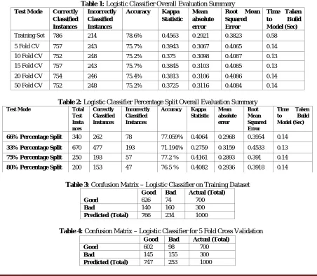
The overall evaluation summary of Logistic Classifier using training set and different cross validation methods is given in Table 1. The classification summary of Logistic Classifier for different percentage split is given in Table 2. The confusion matrix for each different test mode is given in Table 3 to Table 12. Logistic Classifier gives 78.6% for the training data set. But for evaluation testing with test data is essential. So various cross validation and percentage split methods are used to test its actual performance. On an average, it gives around 75% of classification accuracy for credit risk prediction.

Table 1: Logistic Classifier Overall Evaluation Summary

Test Mode Correctly

Classified Instances

Incorrectly Classified Instances

Accuracy Kappa

Statistic Mean absolute error

Root Mean

Squared Error

Time Taken

to Build

Model (Sec)

Training Set 786 214 78.6% 0.4563 0.2921 0.3823 0.58

5 Fold CV 757 243 75.7% 0.3943 0.3067 0.4065 0.14

10 Fold CV 752 248 75.2% 0.375 0.3098 0.4087 0.13

15 Fold CV 757 243 75.7% 0.3845 0.3103 0.4085 0.13

20 Fold CV 754 246 75.4% 0.3813 0.3106 0.4086 0.14

50 Fold CV 752 248 75.2% 0.3725 0.3116 0.4084 0.14

Table 2: Logistic Classifier Percentage Split Overall Evaluation Summary

Test Mode Total Test Insta nces Correctly Classified Instances Incorrectly Classified Instances

Accuracy Kappa Statistic Mean absolute error Root Mean Squared Error

Time Taken to Build Model (Sec)

66% Percentage Split 340 262 78 77.059% 0.4064 0.2968 0.3954 0.14

75% Percentage Split 250 193 57 77.2 % 0.4161 0.2893 0.391 0.14

Table 3: Confusion Matrix – Logistic Classifier on Training Dataset

Good Bad Actual (Total)

Good 626 74 700

Bad 140 160 300

Predicted (Total) 766 234 1000

Table 4: Confusion Matrix – Logistic Classifier for 5 Fold Cross Validation

Good 602 98 700

Bad 145 155 300

(4)

Volume 3, Issue 4, April 2014

Page 58

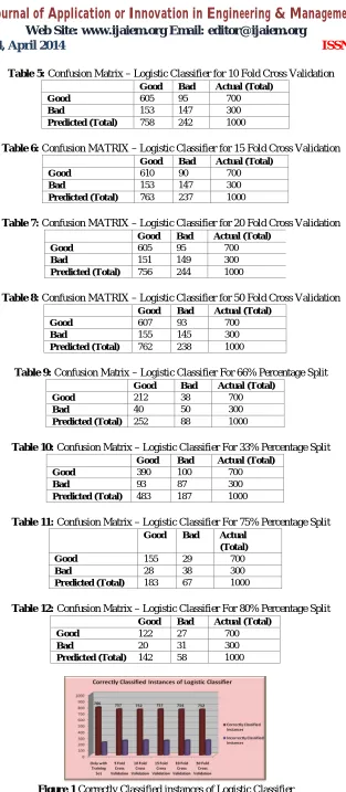
Table 5: Confusion Matrix – Logistic Classifier for 10 Fold Cross Validation

Good 605 95 700

Bad 153 147 300

Table 6: Confusion MATRIX – Logistic Classifier for 15 Fold Cross Validation

Good 610 90 700

Bad 153 147 300

Good 605 95 700

Bad 151 149 300

Good 607 93 700

Bad 155 145 300

Table 9: Confusion Matrix – Logistic Classifier For 66% Percentage Split

Good 212 38 700

Bad 40 50 300

Good 390 100 700

Bad 93 87 300

Good Bad Actual

(Total)

Good 155 29 700

Bad 28 38 300

Good 122 27 700

Bad 20 31 300

(5)

Volume 3, Issue 4, April 2014

Page 59

Figure 2 Classification Accuracy of Logistic Classifier

Figure 3 Classification Accuracy of Logistic Classifier for different Percentage Split

6.2 Performance of SMO Classifier

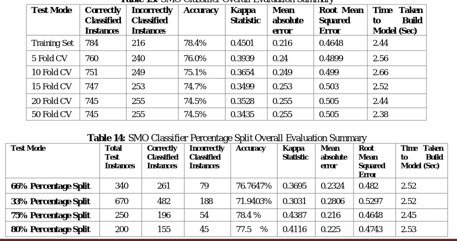
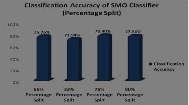
The overall evaluation summary of SMO Classifier using training set and different cross validation methods is given in Table 13. The classification summary of SMO Classifier for different percentage split is given in Table 14. The confusion matrix for each different test mode is given in Table 15 to Table 24. The chart showing the performance of SMO Classifier with respect to Correctly Classified Instances and Classification Accuracy with different type of test modes are depicted in Fig. 4, Fig. 5 and Fig. 6. SMO classifier gives 78.4% for the training data set. But for testing various cross validation and percentage split methods, it performs more or less equal to logistic classifier. On an average, SMO Classifier gives around 75% of classification accuracy for credit risk prediction.

Table 13: SMO Classifier Overall Evaluation Summary

Test Mode Correctly

Classified Instances

Accuracy Kappa

Statistic Mean absolute error

Root Mean Squared Error

Time Taken

to Build

Model (Sec)

Training Set 784 216 78.4% 0.4501 0.216 0.4648 2.44

5 Fold CV 760 240 76.0% 0.3939 0.24 0.4899 2.56

10 Fold CV 751 249 75.1% 0.3654 0.249 0.499 2.66

15 Fold CV 747 253 74.7% 0.3499 0.253 0.503 2.52

20 Fold CV 745 255 74.5% 0.3528 0.255 0.505 2.44

50 Fold CV 745 255 74.5% 0.3435 0.255 0.505 2.38

Table 14: SMO ClassifierPercentage Split Overall Evaluation Summary

Test Mode Total Test Instances

Correctly Classified Instances

Accuracy Kappa Statistic

Mean absolute error

Root Mean Squared Error

Time Taken to Build Model (Sec)

(6)

Volume 3, Issue 4, April 2014

Page 60

Table 15: Confusion Matrix – SMO on Training Dataset

Good 626 74 700

Bad 142 158 300

Table 16: Confusion Matrix – SMO for 5 Fold Cross Validation

Good 610 90 700

Bad 150 150 300

Good 610 90 700

Bad 159 141 300

Good 612 88 700

Bad 165 135 300

Predicted (Total)

777 223 1000

Good 626 74 700

Bad 142 158 300

Good 610 90 700

Bad 150 150 300

Table 21: Confusion Matrix – SMO for66%Percentage Split

Good 218 32 250

Bad 47 43 90

Good 389 101 490

Bad 87 93 180

Good Bad Actual

(Total)

Good 158 26 184

Bad 28 38 66

Good 126 23 149

Bad 22 29 51

(7)

Volume 3, Issue 4, April 2014

Page 61

Figure 4 Correctly Classified instances of SMO Classifier

Figure 5 Classification Accuracy of Logistic Classifier

Figure 6 Classification Accuracy of SMO Classifier for different Percentage Split

6.3 Comparison of Logistic and SMO Classifiers

(8)

Volume 3, Issue 4, April 2014

Page 62

Figure 7 Correctly Classified Instances Comparison between Logistic and SMO Classifier for Percentage Split

Figure 8 Classification Accuracy Comparison between Logistic and SMO Classifier

Figure 9 Classification Accuracy Comparison between Logistic and SMO Classifier for different Percentage Split

7. Conclusion

(9)

Volume 3, Issue 4, April 2014

Page 63

evaluation. After experiment, it is observed that Sequential Minimal Optimization (SMO) Classifier performs better than Logistic Classifier for credit risk prediction.

References

[1] John C. Platt, “Fast Training of Support Vector Machines using Sequential Minimal Optimization,” 2000.

[2] Germano C. Vasconcelos, Paulo J. L. Adeodato and Domingos S. M. P. Monteiro, “A Neural Network Based Solution for the Credit Risk Assessment Problem,” Proceedings of the IV Brazilian Conference on Neural Networks - IV Congresso Brasileiro de Redes Neurais pp. 269-274, July 20-22, 1999.

[3] Tian-Shyug Lee, Chih-Chou Chiu, Chi-Jie Lu and I-Fei Chen, “Credit scoring using the hybrid neural discriminant technique,” Expert Systems with Applications (Elsevier) 23, pp. 245–254, 2002.

[4] Zan Huang, Hsinchun Chena, Chia-Jung Hsu, Wun-Hwa Chen and Soushan Wu, “Credit rating analysis with support vector machines and neural networks: a market comparative study,” Decision Support Systems (Elsevier) 37, pp. 543– 558, 2004.

[5] Kin Keung Lai, Lean Yu, Shouyang Wang, and Ligang Zhou, “Credit Risk Analysis Using a Reliability-Based Neural Network Ensemble Model,” S. Kollias et al. (Eds.): ICANN 2006, Part II, Springer LNCS 4132, pp. 682 – 690, 2006.

[6] Eliana Angelini, Giacomo di Tollo, and Andrea Roli “A Neural Network Approach for Credit Risk Evaluation,” Kluwer Academic Publishers, pp. 1 – 22, 2006.

[7] S. Kotsiantis, “Credit risk analysis using a hybrid data mining model,” Int. J. Intelligent Systems Technologies and Applications, Vol. 2, No. 4, pp. 345 – 356, 2007.

[8] Hamadi Matoussi and Aida Krichene, “Credit risk assessment using Multilayer Neural Network Models - Case of a Tunisian bank,” 2007.

[9] Lean Yu, Shouyang Wang, Kin Keung Lai, “Credit risk assessment with a multistage neural network ensemble learning approach”, Expert Systems with Applications (Elsevier) 34, pp.1434–1444, 2008.

[10]Arnar Ingi Einarsson, “Credit Risk Modeling”, Ph.D Thesis, Technical University of Denmark, 2008.

[11]Sanaz Pourdarab, Ahmad Nadali and Hamid Eslami Nosratabadi, “A Hybrid Method for Credit Risk Assessment of Bank Customers,” International Journal of Trade, Economics and Finance, Vol. 2, No. 2, April 2011.

[12]Vincenzo Pacelli and Michele Azzollini, “An Artificial Neural Network Approach for Credit Risk Management”, Journal of Intelligent Learning Systems and Applications, 3, pp. 103-112, 2011.

[13]A.R.Ghatge and P.P.Halkarnikar, “Ensemble Neural Network Strategy for Predicting Credit Default Evaluation” International Journal of Engineering and Innovative Technology (IJEIT) Volume 2, Issue 7, January 2013 pp. 223 – 225.

[14]Lakshmi Devasena, C., “Adeptness Evaluation of Memory Based Classifiers for Credit Risk Analysis,” Proc. of International Conference on Intelligent Computing Applications - ICICA 2014, 6-7, (IEEE Explore), March 2014, pp. 143-147.

[15]Lakshmi Devasena, C., “Adeptness Comparison between Instance Based and K Star Classifiers for Credit Risk Scrutiny,” International Journal of Innovative Research in Computer and Communication Engineering, Vol.2, Special Issue 1, March 2014.

[16]Lakshmi Devasena, C., “Adeptness Comparison between Instance Based and K Star Classifiers for Credit Risk Scrutiny,” Proc. of International Conference on Intelligent Computing Applications - ICICA 2014, 978-1-4799-3966-4/14 (IEEE Explore), 6-7 March 2014, pp. 143-147, 2014.

[17]UCI Machine Learning Data Repository – http://archive.ics.uci.edu/ml/datasets.

[18]De Mantaras and Armengol E, ”Machine learning from example: Inductive and Lazy methods”, Data & Knowledge Engineering 25: 99-123, 1998.

AUTHOR

Dr. C. Lakshmi Devasena has completed her Ph.D in Karpagam University, Coimbatore. She has 10 ½ years of Teaching and two years of Industrial experience. She has published 35 papers, in that 24 papers are published in International Journals and 11 are published in National Journals and conference proceedings. She has presented 35 papers in various International and National conferences. Her research interest is Data Mining, Medical Image Analysis, Business Analytics, Evaluation of Algorithms, and E-Governance. She is presently working in Operations & IT Area, IBS Hyderabad, IFHE University.