The Thirty-Third AAAI Conference on Artificial Intelligence (AAAI-19)
Deep Embedding Features for Salient Object Detection
Yunzhi Zhuge,
†Yu Zeng,
†Huchuan Lu
††Dalian University of Technology
†{zgyz, zengyu}@mail.dlut.edu.cn,†[email protected]
Abstract
Benefiting from the rapid development of Convolutional Neu-ral Networks (CNNs), some salient object detection methods have achieved remarkable results by utilizing multi-level con-volutional features. However, the saliency training datasets is of limited scale due to the high cost of pixel-level labeling, which leads to a limited generalization of the trained model on new scenarios during testing. Besides, some FCN-based methods directly integrate multi-level features, ignoring the fact that the noise in some features are harmful to saliency de-tection. In this paper, we propose a novel approach that trans-forms prior information into an embedding space to select attentive features and filter out outliers for salient object de-tection. Our network firstly generates a coarse prediction map through an encorder-decorder structure. Then a Feature Em-bedding Network (FEN) is trained to embed each pixel of the coarse map into a metric space, which incorporates much at-tentive features that highlight salient regions and suppress the response of non-salient regions. Further, the embedded fea-tures are refined through a deep-to-shallow Recursive Feature Integration Network (RFIN) to improve the details of pre-diction maps. Moreover, to alleviate the blurred boundaries, we propose a Guided Filter Refinement Network (GFRN) to jointly optimize the predicted results and the learnable guid-ance maps. Extensive experiments on five benchmark datasets demonstrate that our method outperforms state-of-the-art re-sults. Our proposed method is end-to-end and achieves a real-time speed of 38 FPS.
Introduction
Salient object detection, which aims to estimate the visual significance of image regions, has arisen widely discussions in recent years. It serves as a pre-processing step for many computer vision tasks, such as image regartigating (Fang et al. 2012), image classification (Schmid, Jurie, and Sharma 2012) and quality assessment (Zhang, Shen, and Li 2014). However, due to many uncertain factors such as cluttered backgrounds and complex scenarios, it still remains a diffi-cult task.
Earlier saliency detection methods (Li et al. 2013) (Jiang et al. 2013) generate saliency maps under the guidance of heuristic priors(e.g. color, texture and contrast). However,
Copyright c2019, Association for the Advancement of Artificial Intelligence (www.aaai.org). All rights reserved.
these low-level features can hardly capture high-level se-mantic relations of the objects and its surroundings. Thus the low-level based methods are not robust enough to distin-guish salient objects from cluttered background.
Recently, deep convolutional neural networks have shown outstanding performance in many recognition tasks. Own-ing to its hierarchical structure, CNNs can learn multi-level features from training samples. Compared with the hand-crafted features, the CNNs features are more semantically rich. Therefore, the CNNs based saliency detection meth-ods (Wang et al. 2016; Liu and Han 2016) have achieved impressive results by leveraging high-level semantic fea-tures to capture foreground areas. However, the CNNs based methods still have two apparent deficiencies. On the one hand, downsampling operations such as pooling and con-volution dramatically reduce the resolution of initial image, which degrade the details such as image boundary. On the other hand, many CNNs based methods (Zhang et al. 2017a; Wang et al. 2017b; Zhang et al. 2018a) introduce overloaded layers to integrate multi-level features. Such excessive pro-cesses often cause features cluttered, and thus cause the in-correct saliency detection results.
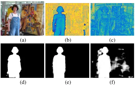
(a) (b) (c)
(d) (e) (f)
Figure 1: Visual comparison with a multi-level feature based method. From top-left to bottom-right: (a) Input image. (b)-(c) Feature maps of our method and Amulet (Zhang et al. 2017a). (d) Ground Truth. (e)-(f) Saliency maps of our method and Amulet.
saliency maps predicted by RFIN. GFRN transforms the original RGB image into a guidance map to refine bound-aries of the salient objects. As is shown in Figure 1, com-pared with an existing method Amulet (Zhang et al. 2017a) based on multi-level features integration, our method can generate more precise saliency map in the guidance of ro-bust feature maps.
In summary, each component in our algorithm plays a role in enhance the accuracy for salient object detection. Our main contributions are as follows:
• Motivated by the aforementioned drawbacks of directly
integrating multi-level features, we suggest to boost salient object detection results in a new point, i.e., embed-ding prior predictions into a metric space to filter outliers and generate attentive features to precisely localize salient objects.
• We propose a Recursive Feature Integration Network
(RFIN) which progressively refines the embedding fea-tures by integrating them with multi-level feafea-tures in a deep-to-shallow sequence.
• The proposed method achieves state-of-the-art results on
five large-scale benchmark datasets. It also achieves a real-time speed of 38 FPS using one 1080 Ti GPU.
Related Work
Over the past decades, a large set of saliency detection meth-ods have been developed. Saliency detection methmeth-ods can be roughly divided into two categories: methods based on hand-crafted features and deep learning based methods.
Methods Based on Hand-crafted Features
Earlier saliency detection methods mainly focused on ex-ploiting hand-crafted features, which can be categorized as local and global schemes. Local methods measure local-contrast to evaluate saliency. In (Sch¨olkopf, Platt, and Hof-mann 2006), the equilibrium distribution over map locations are treated as activation and saliency values. In contrast,
ISP
FRMs
64 x 64 x 64 64 x 64 x 64 64 x 64 x 64 64 x 64 x 64 64 x 64 x 64
64 x 64 x (64x5)
identity
Feature embeddings
Distance calculation
Feature subtraction
conv 64 x 64
x 256
ELM
RFIN
Figure 2: The structure of Feature Embedding Network.
global methods considering both color statistics and holis-tic contrast of the whole image. In (Liu et al. 2011), condi-tional random field is learned to effectively combine local and global features for saliency detection. (Jiang et al. 2013) propose a method to map the regional feature vector to a saliency score using Random Forest regressor. (Cheng et al. 2011) utilize color-discriminative features and global con-trast to obtain optimal saliency maps.
Deep Learning Based Methods
Recently, deep convolutional neural networks (CNNs) have delivered superior performance in many recognition tasks (Krizhevsky, Sutskever, and Hinton 2012; He et al. 2016). In earlier research (Wang et al. 2015; Li and Yu 2015; Zhao et al. 2015), image patches are the basic processing unit for saliency prediction. Although these algorithms per-form superior than hand-crafted feature based methods, they are relatively sparse in spatial and time-consuming due to the fully connected layers. To resolve this problem, sev-eral attempts based on fully convolutional networks (FCNs) are proposed. (Liu and Han 2016) propose a deep hierar-chical network that progressively refine saliency maps by integrating local context information. (Wang et al. 2016) take predicted saliency maps as input to recurrently refine the generated saliency maps by rectify its previous errors. In (Hou et al. 2017), short connections are proposed to con-vert high-level features into shallower layers, which locate salient regions and refine the sparse details simultaneously. (Zhang et al. 2017a) integrate and combine multi-level fea-ture maps to simultaneously incorporate coarse semantics and fine details. (Wang et al. 2017b) propose a stage-wise refinement model with a pyramid pooling to extract global context information and local details for salient object de-tection. (Zhang et al. 2018b) firstly denote that some fea-tures are redundant for salient object detection. An attention guided network is proposed to selectively integrates multi-level contextual information and alleviate distraction of clut-tered features. Different from the above feature integration based methods, we propose a multi-branch deep embedding feature network which can simultaneously map coarse pre-diction map into a metric space and incorporate multiple side output features recursively to exploits both global and local information.
Feature Embedding
C
C
C
Conv-1 128 x 128 x 64
res-2 64 x 64 x 256
res-3 32 x 32 x 512
res-4 16 x 16 x 1024
res-5 16 x 16 x 2048
ISP 64 x 64 x 1 ELM
64 x 64 x 256 FRM5 64 x 64 x 64
FRM4 64 x 64 x 64
FRM3 64 x 64 x 64
FRM2 64 x 64 x 64
FRM1 64 x 64 x 64
RFRM1 64 x 64 x 256
RFRM2 64 x 64 x 256
RFRM3 64 x 64 x 256
RFRM4 64 x 64 x 256
SSP
64 x 64 x 1
SSP
64 x 64 x 1
SSP
64 x 64 x 1 SSP/Upsample
256 x 256 x 1 GFRN
Stimuli GT Predicted Map
C
InformationStream Multi-information
Stream
Addition
Concatenation
FEN
R
FI
N
Backbone
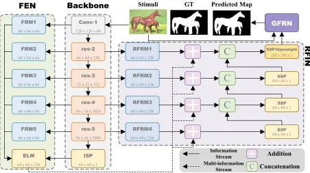
Figure 3: The pipeline of our method. Each module or block is presented by a solid box.FEN−Feature Embedding Network.
RFIN−Recursive Feature Integration Network.GFRN−Guided Filter Refinement Network.ISP−Initial Saliency
Predic-tion.SSP−Stagewise Saliency Prediction.FRM−Feature Reshape Module.RFRM−Residual Feature Reshape Module.
ELM−Embedding Learning Module.
features into high-level features, which leverages the advan-tage of CNNs to simultaneously capture semantic informa-tion in high-level features as well as spatial and contrast in-formation in low-level features. In (Liu et al. 2018), a fully convolutional network is trained to learn the feature ding space for each superpixel. The learned feature embed-ding corresponds to a similarity measure between two ad-jacent superpixels. In (Zeng et al. 2018), an image-specific classifier is learned from the attributes of training data to classify the pixels of each image.
Different from the above embedding methods, our deep feature embedding network transforms both the prior pre-dictions and multi-level features into a metric space. With the help of the prior information about the salient regions, the generated attentive features can effectively hightlight the salient regions and suppress the backgrounds.
Proposed Method
We describe the proposed method in this section. To begin with, we describe the components of our proposed DEF ar-chitecture in the first subsection. Then we explain the de-tailed training schemes of our algorithms in the last subsec-tion.
Architecture
The main architecture of our proposed algorithm is shown in Figure 3. It is a multi-branch network consisting of four components: Initial Saliency Network (ISN), Deep Feature Embedding Network (FEN), Recursive Feature Integration
Network (RFIN) and Guided Filter Refinement Network (GFRN). ISN provides the initial saliency predictions and multi-scale side output features. FEN embeds the predic-tions and features of ISN into a metric space to weight the spatial importance of each element in feature maps. RFIN integrates embedded features with residual reconstructed features and predicts a series of stage-wise saliency maps in deep-to-shallow manner. GFRN takes original RGB im-age and the last saliency map produced by RFIN as inputs. The RGB image is transformed into a guidance map to refine boundaries of the salient objects.
Initial Saliency Network We format our Initial Saliency
Network on the basis of fully convolutional network. We choose ResNet101 (He et al. 2016) as our backbone due to its fast convergence characteristic and astonishing results in image classification task. ResNet101 is composed of five ba-sic blocks with different output dimensions: conv1, res2, res3,res4, andres5. The output spatial of basic blocks are
decreased by a stride of 2. To obtain larger feature maps, we set the stride of the last block to 1. For computation effi-ciency, we choose the output of last two blocks as side output
layers, denoted asSide4andSide5. To reduce dimensions,
we pass them through two convolution layers with 256 ker-nels. The initial prediction map are produced by feeding the two feature maps into a convolution layer with 1 kernels and
upsampled to64×64.
Feature Embedding Network After obtaining the initial
64 x 64 x 256 64 x 64
x 256
64 x 64 x 256
64 x 64 x 128
H x W x C
64 x 64 x 256
Figure 4: Overall architecture of Residual Feature Reshape Module.
Feature Embedding Network (FEN) to map the features and initial prediction maps into a metric space. FEN is composed of paralleled Feature Reshape Modules (FRM) and Embed-ding Learning Module (ELM), As is shown in Figure 2. To begin with, we utilize Feature Reshape Modules to integrate multi-level feature maps. Features of different spatial resolu-tions are resized into the same scale through pooling or up-sampling operations. Then we use a convolutional layer with
64 kernels to reduce dimensions. LetSideldenotes feature
maps of levell(l = 1,2, ...,5). All feature maps are resized
to the same spatial size of64×64. The integrated feature
maps are generated by
F =Cat5l=1(Conv(Sidel))), (1)
in whichConvandCatdenotes convolution and
concatena-tion operaconcatena-tion respectively. The resulting integrated feature
map is of the shape64×64×320, where64×64represents
spatial size and320represents number of channels.
Denotexmas a pixel of imageXin positionm. Given an
initial saliency map S1, we first obtain a reverse saliency
map S0 by S0 = 1 - S1 that highlights background area.
Then, each pixel of saliency and reverse saliency maps is
mapped into a320-dimensional vector by
ϕmk =µ(smk;ψ), k= 0,1, (2)
wheresmkis the value ofSk in positionm.ϕm1andϕm0
are the embedding vector of the pixel in position m of
saliency map and the reverse saliency map, respectively.µ
andψrepresents embedding operation and its parameter.
Given an imageI, we obtain the attentive features of the
pixel in positionmaccording to:
V(Im) =|Dis(ϕm1,fm)−Dis(ϕm0,fm)|, (3)
wherefmdenotes vector of integrated feature maps in
posi-tionm.Dis(·,·)denotes Euclidean distance.
Recursive Feature Integration Network The Feature
Embedding Network effectively embeds saliency maps into metric space to generate attentive features. Though we can directly apply a softmax layer to obtain relatively precise prediction saliency maps, some detailed areas are still ig-nored. Therefore, we propose a Recursive Feature Integra-tion Network to supplement detailed informaIntegra-tion.
Input Saliency Map
Stimuli
Output Saliency Map
G Mean Filter
Linear Layer
Linear Model G
S
A b
r
Figure 5: Computation process of Guided Filter Refinement Network. GFRN takes original image and saliency map gen-erated by last step as inputs, generating refined saliency map
with sharp boundary.−→represents forward stream and99K
represents back propagation.
As is shown in Figure 3, Recursive Feature Integration
Network takes embedded feature mapsEmand multi-scale
features as input. To begin with, Residual Feature Reshape Module (RFRM) is proposed to reconstruct side-output fea-tures to facilitate it for further integration (depicted in Fig-ure 4). Assume that the spatial size of input featFig-ures is
(RH×W×C), we utilize two paralleled convolution layers to
reshape features and learn complementary information for integration. In each step, RFIN learns to supplement details of embedded feature maps and rectify prediction results of
the last step. The stage-wise saliency predictions of step i
can be produced by:
Pi= (
Wi∗Cat((Em+RFRl),Pi−1) +b,i = 2,3,4
Wi∗(Em+RFRl) +b,i= 1
(4)
where * andWi represents convolution operation and its
parameters to generate prediction maps. RFRl represents
the feature maps generated by RFIN at levell.bis the bias parameter. In Equation 4, The stagewise prediction results in leveli(i= 2,3,4)is obtained by integrating corresponding
RFIN features andi−1prediction maps.
Guided Filter Refinement Network The RFIN can
gen-erate finer results by recursively integrate embedded maps and multi-level features. However, due to the down-sampling operation of base network, there still exists a gap between prediction results and ground truth, especially on object boundaries. To further refine details and make the boundary clear of salient objects, we adopt a Guided Filter Refinement Network (GFRN) (Wu et al. 2018) to overcome the bondage of the base network.
The computation process of GFRN is shown in Figure 5. The original RGB image and the saliency map generated by RFIN are the input of GFRN. Given a pair of inputs, convo-lutional layers are first added as a transformation function to change the dimension of input image, which serves as a flex-ible and trainable guidance map. After that, GFRN computes
Aandbby minimizing the reconstruction error betweenG
and S with mean filter and linear model. Output saliency
map (O) is computed by an linear transformation takingA,
bandGas inputs:
(a) (b) (c) (d) (e) (f)
Figure 6: Visual comparison of several components. From left to right: (a)Image, (b)Ground Truth, (c)Baseline, (d)FEN, (e)RFIN(stage-4), (f)GFRN.
randεrepresents radius of mean filter and the regularization term respectively.
Training Schemes
Our proposed multi-branch model is trained end-to-end.
In-put images are resized to256×256to match the size
re-quirements of base network. During training, initial saliency maps generated by Initial Saliency Network are inaccurate, which effect the performance of our algorithm. To get rid of this deficiency, during training we randomly disarray the pixel of ground truth with a certain probability and serves it as input to the Feature Embedding Network (FEN). To train the model, we minimize the cross-entropy loss between each stage-wise prediction of RFIN and the ground-truth, as well as the cross-entropy loss between the final output and the groud-truth.
Experiments
To verify the effectiveness of our proposed algorithm, we conduct experiments on five public datasets (ECSSD, PASCAL-S, DUT-OMRON, DUTS and HKU-IS). We eval-uate the proposed algorithm using precision-recall curves (PR-curves), mean F-measure, mean absolute error (MAE). In addition, we briefly explain the implementation details of our method and evaluate the performance of our method by comparing with other state-of-the-arts algorithms.
Implementation details
We implement our approach in Python with the Pytorch tool-box. We run our approach on a PC with a 3.7GHz CPU, 32GB RAM and a GTX 1080 Ti GPU (with 11G memory).
We train our model using DUTS training dataset (Wang et al. 2017b). To avoid over-fitting, we augment the training set by 4 times through horizontal flipping and vertical flipping. We use SGD to optimize our network with the momentum parameter of 0.9 and the weight decay of 0.001. We set the base learning rate to 1e-7 and iteration number to 30K. It takes around 7 hours to train our model with a mini-batch of 10. When testing, the proposed algorithm takes around
0.026 second (38FPS) to process an image with256×256
resolution.
Datasets and Evaluation Metrics
To evaluate the performance of our proposed methods, we adopt five benchmark datasets as follows.
ECSSD(Yan et al. 2013) is composed of 1000 images
with multiple objects of different scales. This dataset con-tains many semantically meaningful and complex structures contends.
PASCAL-S(Li et al. 2014) is derived from PASCAL
VOC2010 segmentation dataset (Everingham 2008) and contains 850 natural images.
HKU-IS (Li and Yu 2015) includes 4447 images with
fined pixel-wise annotations. Images of this dataset are well chosen to include multiple disconnected salient objects or objects touching the image boundary.
DUTS (Wang et al. 2017a) is a large dataset which is
composed of 10553 training images and 5019 test images with accurate pixel-wise annotations. All training images are picked out from the ImageNet DET training/val sets, while test images are picked out from the ImageNet DET test set and the SUN dataset.
DUT-OMRON(Yang et al. 2013) has a total of 5168
high-quality images. These images are chosen from more than 140,000 natural images, each of which contains one or more salient objects and relatively complex backgrounds. Thus this dataset is more difficult and challenging, and pro-vides more space of improvement for related research in saliency detection.
Evaluation Metrics. We evaluate the performance of
different salient object detection algorithms through three main metrics, including the precision-recall curves (PR curves), F-measure, mean absolute error(MAE). PR curves can be computed by binarizing the saliency map with a
threshold in [0,255] and then comparing the binary maps
with the ground truth. To be specific, precision represents the percentage of salient pixels being correctly detected, while recall corresponds to the ratio between properly detected salient pixels and salient pixels in ground truth. In many occasions, both precision and recall are important measure metrics. Therefore F-measure, which is calculated by preci-sion and recall, is used as an overall performance measure,
Fβ=
(1 +β2)×P recision×Recall
β2×P recision+Recall . (6)
We setβ2to 0.3 to emphasize the precision. And MAE score
can be calculated by average pixel-wise absolute difference between the binary ground truth and the saliency map:
T= 1
W ×H
W
X
x=1 H
X
y=1
|S(x, y)−G(x, y)|, (7)
where W and H denote width and height of an image, S(x, y)is the saliency value of the pixel at(x, y).
Comparison with State-of-the-arts
0 0.2 0.4Recall0.6 0.8 1 0.2 0.3 0.4 0.5 0.6 0.7 0.8 0.9 1 Precision ECSSD BSCA DRFI MDF LEGS ELD DCL DS RFCN NLDF DHS UCF Amulet SRM BPN Ours
0 0.2 0.4Recall0.6 0.8 1 0.2 0.3 0.4 0.5 0.6 0.7 0.8 0.9 1 Precision PASCAL-S BSCA DRFI MDF LEGS ELD DCL DS RFCN NLDF DHS UCF Amulet SRM BPN Ours
0 0.2 0.4Recall0.6 0.8 1 0.2 0.3 0.4 0.5 0.6 0.7 0.8 0.9 1 Precision HKU-IS BSCA DRFI MDF LEGS ELD DCL DS RFCN NLDF DHS UCF Amulet SRM BPN Ours
0 0.2 0.4Recall0.6 0.8 1 0.2 0.3 0.4 0.5 0.6 0.7 0.8 0.9 1 Precision DUT-OMRON BSCA DRFI MDF LEGS ELD DCL DS RFCN NLDF UCF Amulet SRM BPN Ours
0 0.2 0.4Recall0.6 0.8 1 0.2 0.3 0.4 0.5 0.6 0.7 0.8 0.9 1 Precision DUTS-TE BSCA DRFI MDF LEGS ELD DCL DS RFCN NLDF DHS UCF Amulet SRM BPN Ours
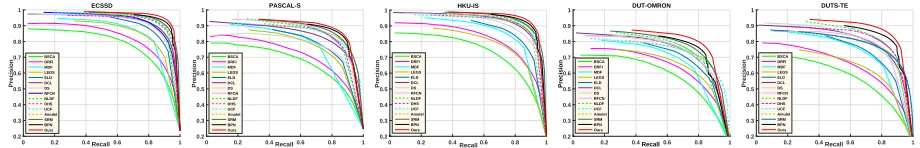
Figure 7: Precision-Recall curves of our method and other state-of-art methods on five benchmark datasets.
Table 1: The mean F-measure (larger is better) and MAE (smaller is better) of different saliency detection methods on five saliency detection datasets. The best three results are shown in bold, italic, and underlined. Our method ranks first on most of these datasets and metrics.
Method ECSSD PASCAL-S HKU-IS DUT-OMRON DUTS-TE
Fβ MAE Fβ MAE Fβ MAE Fβ MAE Fβ MAE
Ours 0.915 0.036 0.826 0.070 0.907 0.033 0.769 0.062 0.821 0.045 BPN (Wang et al. 2018) 0.903 0.045 0.816 0.074 0.882 0.038 0.708 0.063 0.763 0.052 SRM (Wang et al. 2017b) 0.892 0.056 0.821 0.085 0.874 0.046 0.707 0.069 0.757 0.059 Amulet (Zhang et al. 2017a) 0.867 0.059 0.763 0.100 0.839 0.052 0.648 0.098 0.676 0.085 UCF (Zhang et al. 2017b) 0.841 0.080 0.701 0.127 0.808 0.074 0.613 0.132 0.629 0.117 DHS (Liu and Han 2016) 0.871 0.063 0.773 0.095 0.852 0.054 - - 0.724 0.067 NLDF (Luo et al. 2017) 0.878 0.063 0.814 0.099 0.873 0.048 0.683 0.079 0.743 0.065 RFCN (Wang et al. 2016) 0.834 0.109 0.751 0.133 0.835 0.089 0.627 0.111 0.712 0.067 DS (Li et al. 2015b) 0.826 0.124 0.659 0.176 0.785 0.078 0.603 0.120 0.632 0.091 DCL (Li and Yu 2015) 0.805 0.108 0.709 0.146 - - 0.644 0.092 0.673 0.101 ELD (Lee, Tai, and Kim 2016) 0.810 0.082 0.718 0.123 0.769 0.074 0.611 0.092 0.628 0.093 LEGS (Wang et al. 2015) 0.785 0.118 0.699 0.158 0.723 0.119 0.591 0.133 0.585 0.138 MDF (Li et al. 2015b) 0.807 0.105 0.709 0.146 0.801 0.089 0.644 0.092 0.673 0.094 DRFI (Jiang et al. 2013) 0.733 0.164 0.618 0.206 0.722 0.144 0.550 0.139 0.541 0.175 BSCA (Qin et al. 2015) 0.705 0.185 0.601 0.223 0.654 0.175 0.509 0.190 0.499 0.197
al. 2015), MDF (Li and Yu 2015)) and two conventional al-gorithms (DRFI (Jiang et al. 2013), BSCA(Qin et al. 2015)). For fair comparison, we compute other saliency maps with their original implementation details or use them provided by the authors.
Quantitative Evaluation We compare the proposed
method with the others in terms of PR curves, F-measure scores and MAE scores. Figure 7 shows the proposed ap-proach performs favorably against all the other methods. MAE scores and F-measure scores are given in Table 1. As we can see, our approach generates the best score across all datasets, which means that our method have a good perceive of salient region and can generate accurate saliency maps close to the ground truth masks.
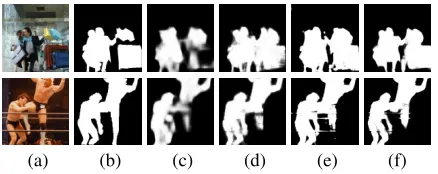
Visual Comparison Figure 8 shows the visual
compar-isons of our approach and other methods. In the shown ex-amples, we accurately segment the salient objects against multiple interference, including rare pattern (row 1), low contrast (row 2&row 5), high-level semantic information (row 4) and complex background (row 6). From these com-parisons, we can see that our method can generate more ac-curate saliency maps with purity backgrounds.
Ablation Studies
The proposed framework is composed of four components, including ISN, FEN, RFIN and GFRN. To show the effec-tiveness of each component, we take a series experiments
on ECSSD and DUTS-TE datasets as follows. We take F-measure and MAE scores as evaluating indicators.
Effectiveness of Each Components We set the results of
ISN as our baseline version. To demonstrate the
effective-ness of Feature Embedding Network, we add a 1
dimen-sion convolution layer to predict saliency maps based on the embedding features, denoted as FEN. The result of FEN shown in row 3 of Table 2 demonstrates that deep embedding features can effectively enhance the localization and detec-tion capability of the saliency detector. As is shown in Fig-ure 3, Recursive FeatFig-ure Integration Network (RFIN) totally generates 4 stage-wise saliency predictions in one pass. We analyze the effectiveness of Recursive Feature Integration by comparison these stage-wise results. For notation sim-plicity, we denoteL(L = 1,2,3,4)stage results as RFIN
(stage-L). Comparison results are shown in rows 4-7 of
Ta-ble 2. Through recursively feature integration, our algorithm can produce more and more accurate results, which demon-strate that by recursively integrate the side-output features and stage-wise predictions, RFIN can effectively reduce the error of last stage.The 8 row of Table 2 indicates that Guided Filter Refinement Network can still increase the F-measure
score by1%. Visual comparison of several components are
shown in Figure 6
Different Backbones To demonstrate that our proposed
Image GT DEF BPN SRM Amulet UCF DHS NLDF RFCN DS
Figure 8: Visual comparison of our method and other methods. It is clear that our methods generates more accurate saliency maps than others.
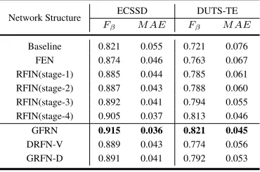
Table 2: Quantitative comparison of different architectures. Baseline denotes the Initial Saliency Prediction. “FEN” in row 3 represents the direct prediction results of Feature Em-bedding Network. 4-7 rows represent the results of differ-ent stage-wise saliency predictions, which monotonically increase. “GFRN”, denotes the prediction results of Gated Feature Refinement Network, which is our final version. The last three rows are comparisons between different back-bones.
Network Structure ECSSD DUTS-TE Fβ M AE Fβ M AE
Baseline 0.821 0.055 0.721 0.076 FEN 0.874 0.046 0.763 0.067 RFIN(stage-1) 0.885 0.044 0.785 0.061 RFIN(stage-2) 0.887 0.043 0.788 0.060 RFIN(stage-3) 0.892 0.041 0.794 0.055 RFIN(stage-4) 0.905 0.037 0.813 0.046 GFRN 0.915 0.036 0.821 0.045
DRFN-V 0.889 0.043 0.774 0.056 GRFN-D 0.891 0.041 0.792 0.053
with two other networks as backbone, i.e. VGG-16 and DenseNet-161. For VGG-16 version, we take 5 feature maps to constitute multi-level features in our work, which are conv1-2,conv2-2,conv3-3,conv4-3andconv5-3,
respec-tively. For DenseNet-161 version, we extract features in the
last layer of each denseblock, we denote them asdense1,
dense2, dense3 and dense4. We keep other settings
un-changed to control variable. The results of both versions are shown in Table 2. From comparing the results of last three rows, we can observe that the proposed method works well for different backbones.
Conclusion
In this paper, we propose a novel deep embedding feature network for salient object detection. Different from existing methods which directly fused multi-level features to gener-ate the prediction maps, we put forward an embedding learn-ing architecture to embed initial saliency map into feature vectors and recursively narrow the gap between stage-wise predictions and ground truth. A Convolutional Guided Fil-ter is also utilized to strengthen overall performance. Exten-sive evaluations demonstrate that our approach achieves the state-of-the-art results. Except for the salient object detec-tion, our DEF possesses the potential of dealing with other low-level vision tasks.
Acknowledgement
This work was supported by the Natural Science Founda-tion of China under Grant 61725202, 61751212, 61771088, 61632006 and 91538201.
References
Cheng, M. M.; Mitra, N. J.; Huang, X.; Torr, P. H. S.; and Hu, S. M. 2011. Global contrast based salient region detection. InProc. of IEEE Conference on Computer Vision and Pattern Recognition, 409–416.
Everingham, M. 2008. The pascal visual object classes chal-lenge 2008 ( voc2008 ) development kit. International Journal of Computer Vision111(1):98–136.
Fang, Y.; Chen, Z.; Lin, W.; and Lin, C. W. 2012. Saliency de-tection in the compressed domain for adaptive image retarget-ing. IEEE Transactions on Image Processing21(9):3888–3901.
Hou, Q.; Cheng, M.-M.; Hu, X.; Borji, A.; Tu, Z.; and Torr, P. 2017. Deeply supervised salient object detection with short
con-nections. InProc. of IEEE Conference on Computer Vision and
Pattern Recognition, 5300–5309. IEEE.
Jiang, H.; Wang, J.; Yuan, Z.; Wu, Y.; Zheng, N.; and Li, S. 2013. Salient object detection: A discriminative regional feature integration approach. InProc. of IEEE Conference on Computer Vision and Pattern Recognition, 2083–2090.
Krizhevsky, A.; Sutskever, I.; and Hinton, G. E. 2012. Imagenet classification with deep convolutional neural networks. In Ad-vances in Neural Information Processing Systems, 1097–1105.
Lee, G.; Tai, Y. W.; and Kim, J. 2016. Deep saliency with en-coded low level distance map and high level features. InProc. of IEEE Conference on Computer Vision and Pattern Recognition,
660–668.
Li, G., and Yu, Y. 2015. Visual saliency based on multiscale deep features. InProc. of IEEE Conference on Computer Vision and Pattern Recognition, 5455–5463.
Li, G., and Yu, Y. 2016. Deep contrast learning for salient object detection. InProc. of IEEE Conference on Computer Vision and Pattern Recognition, 478–487.
Li, X.; Lu, H.; Zhang, L.; Xiang, R.; and Yang, M. H. 2013. Saliency detection via dense and sparse reconstruction. InProc. of IEEE International Conference on Computer Vision, 2976–
2983.
Li, Y.; Hou, X.; Koch, C.; Rehg, J. M.; and Yuille, A. L. 2014.
The secrets of salient object segmentation. In Proc. of IEEE
Conference on Computer Vision and Pattern Recognition, 280–
287.
Li, H.; Lu, H.; Lin, Z.; Shen, X.; and Price, B. 2015a. Lcnn: Low-level feature embedded cnn for salient object detection. Li, X.; Zhao, L.; Wei, L.; Yang, M. H.; Wu, F.; Zhuang, Y.; Ling, H.; and Wang, J. 2015b. Deepsaliency: Multi-task deep neural network model for salient object detection. IEEE Transactions on Image Processing25(8):3919.
Liu, N., and Han, J. 2016. Dhsnet: Deep hierarchical saliency network for salient object detection. InProc. of IEEE Confer-ence on Computer Vision and Pattern Recognition, 678–686.
Liu, T.; Yuan, Z.; Sun, J.; Wang, J.; Zheng, N.; Tang, X.; and Shum, H. Y. 2011. Learning to detect a salient object.
IEEE Transactions on Pattern Analysis & Machine Intelligence
33(2):353–367.
Liu, Y.; Jiang, P.-T.; Petrosyan, V.; Li, S.-J.; Bian, J.; Zhang, L.; and Cheng, M.-M. 2018. Del: Deep embedding learning for efficient image segmentation. InProc. of International Joint Conference on Artificial Intelligence (IJCAI).
Luo, Z.; Mishra, A.; Achkar, A.; Eichel, J.; Li, S.; and Jodoin, P. M. 2017. Non-local deep features for salient object detection. InProc. of IEEE Conference on Computer Vision and Pattern Recognition, 6593–6601.
Qin, Y.; Lu, H.; Xu, Y.; and Wang, H. 2015. Saliency detection via cellular automata. InProc. of IEEE Conference on Computer Vision and Pattern Recognition, 110–119.
Sch¨olkopf, B.; Platt, J.; and Hofmann, T. 2006. Graph-based visual saliency. InAdvances in Neural Information Processing Systems, 545–552.
Schmid, C.; Jurie, F.; and Sharma, G. 2012. Discriminative spa-tial saliency for image classification. InProc. of IEEE Confer-ence on Computer Vision and Pattern Recognition, 3506–3513.
Wang, L.; Lu, H.; Xiang, R.; and Yang, M. H. 2015. Deep networks for saliency detection via local estimation and global
search. InProc. of IEEE Conference on Computer Vision and
Pattern Recognition, 3183–3192.
Wang, L.; Wang, L.; Lu, H.; Zhang, P.; and Xiang, R. 2016. Saliency detection with recurrent fully convolutional networks. InProc. of European Conference on Computer Vision, 825–841.
Wang, L.; Lu, H.; Wang, Y.; Feng, M.; Wang, D.; Yin, B.; and Ruan, X. 2017a. Learning to detect salient objects with
image-level supervision. InProc. of IEEE Conference on Computer
Vision and Pattern Recognition, 3796–3805.
Wang, T.; Borji, A.; Zhang, L.; Zhang, P.; and Lu, H. 2017b. A stagewise refinement model for detecting salient objects in images. InProc. of IEEE International Conference on Computer Vision, 4039–4048.
Wang, T.; Zhang, L.; Wang, S.; Lu, H.; Yang, G.; Ruan, X.; and Borji, A. 2018. Detect globally, refine locally: A novel approach to saliency detection. InProc. of IEEE Conference on Computer Vision and Pattern Recognition, 3127–3135.
Wu, H.; Zheng, S.; Zhang, J.; and Huang, K. 2018. Fast end-to-end trainable guided filter. InProc. of IEEE Conference on Computer Vision and Pattern Recognition, 6450–6458.
Yan, Q.; Xu, L.; Shi, J.; and Jia, J. 2013. Hierarchical saliency detection. InProc. of IEEE Conference on Computer Vision and Pattern Recognition, 1155–1162.
Yang, C.; Zhang, L.; Lu, H.; Xiang, R.; and Yang, M. H. 2013. Saliency detection via graph-based manifold ranking. InProc. of IEEE Conference on Computer Vision and Pattern Recognition,
3166–3173.
Zeng, Y.; Lu, H.; Zhang, L.; Feng, M.; and Borji, A. 2018. Learning to promote saliency detectors. InProc. of IEEE Con-ference on Computer Vision and Pattern Recognition, 38–56.
Zhang, P.; Wang, D.; Lu, H.; Wang, H.; and Ruan, X. 2017a. Amulet: Aggregating multi-level convolutional features for salient object detection. In Proc. of IEEE International Con-ference on Computer Vision, 202–211.
Zhang, P.; Wang, D.; Lu, H.; Wang, H.; and Yin, B. 2017b. Learning uncertain convolutional features for accurate saliency
detection. InProc. of IEEE International Conference on
Com-puter Vision, 212–221.
Zhang, L.; Dai, J.; Lu, H.; He, Y.; and Wang, G. 2018a. A bi-directional message passing model for salient object detection. InProc. of IEEE Conference on Computer Vision and Pattern Recognition, 1741–1750.
Zhang, X.; Wang, T.; Qi, J.; Lu, H.; and Wang, G. 2018b. Pro-gressive attention guided recurrent network for salient object
de-tection. InProc. of IEEE Conference on Computer Vision and
Pattern Recognition, 248–255.
Zhang, L.; Shen, Y.; and Li, H. 2014. Vsi: A visual
saliency-induced index for perceptual image quality assessment. IEEE
Transactions on Image Processing23(10):4270–4281.