Linear Kernel Tests via Empirical Likelihood for High-Dimensional Data

(1)

The Thirty-Third AAAI Conference on Artificial Intelligence (AAAI-19)

Linear Kernel Tests via Empirical Likelihood for High-Dimensional Data

Lizhong Ding,

1,∗

Zhi Liu,

3

Yu Li,

2

Shizhong Liao,

4

Yong Liu,

5

Peng Yang,

2

_{Ge Yu,}

6

_{Ling Shao,}

1

_{Xin Gao}

2,∗

1_{Inception Institute of Artificial Intelligence (IIAI), Abu Dhabi, UAE}

2_{King Abdullah University of Science and Technology (KAUST), Saudi Arabia}

3_{University of Macau, China,}4_{Tianjin University, China,}5_{Institute of Information Engineering, CAS, China}

6_{Technology and Engineering Center for Space Utilization, CAS, China}

∗_{Corresponding authors (email: [email protected], [email protected])}

Abstract

We propose a framework for analyzing and comparing dis-tributions without imposing any parametric assumptions via empirical likelihood methods. Our framework is used to study two fundamental statistical test problems: the two-sample test and the goodness-of-fit test. For the two-sample test, we need to determine whether two groups of samples are from differ-ent distributions; for the goodness-of-fit test, we examine how likely it is that a set of samples is generated from a known target distribution. Specifically, we propose empirical likeli-hood ratio (ELR) statistics for the two-sample test and the goodness-of-fit test, both of which are of linear time complex-ity and show higher power (i.e., the probabilcomplex-ity of correctly rejecting the null hypothesis) than the existing linear statis-tics for high-dimensional data. We prove the nonparametric Wilks’ theorems for the ELR statistics, which illustrate that the limiting distributions of the proposed ELR statistics are chi-square distributions. With these limiting distributions, we can avoid bootstraps or simulations to determine the threshold for rejecting the null hypothesis, which makes the ELR statis-tics more efficient than the recently proposed linear statistic, finite set Stein discrepancy (FSSD). We also prove the con-sistency of the ELR statistics, which guarantees that the test power goes to 1 as the number of samples goes to infinity. In addition, we experimentally demonstrate and theoretically analyze that FSSD has poor performance or even fails to test for high-dimensional data. Finally, we conduct a series of ex-periments to evaluate the performance of our ELR statistics as compared to state-of-the-art linear statistics.

Introduction

Comparing samples from two probability distributions or evaluating the goodness-of-fit of models over observed sam-ples without imposing any parametric assumptions on their distributions are fundamental tasks in machine learning and statistics, and have a wide spectra of applications in var-ious areas (Lloyd and Ghahramani 2015; Li et al. 2017; Yang et al. 2018). The goal of the two-sample test problem is to determine whether two distributionspandqare differ-ent on the basis of samplesDx ={xi}ni=1 ⊂ X ⊆ Rdand

Dy={yj}mj=1⊂ Y ⊆Rdindependently drawn frompand

q, respectively. The aim of the goodness-of-fit test problem is to determine how well a given model densitypfits a set of

given samplesDx={xi}ni=1⊂ X ⊆R

d_{from an unknown}

distributionq. Both of these two problems can be formulated as a hypothesis test, where the null hypothesisH0 :p =q is tested against the alternative hypothesisH1:p6=q. The knowledge ofpis what distinguishes the goodness-of-fit test from the two-sample test.

The two-sample test and the goodness-of-fit test are gen-erally difficult in practice, since the underlying distributions (or one of the distributions) are unknown apriori. Kernel methods provide an effective way to implicitly transform data into a new feature space with the carefully-chosen ker-nel functions and kerker-nel parameters (Liu and Liao 2015; Liu et al. 2017; Ding and Liao 2014a; 2017; Ding et al. 2019). The corresponding reproducing kernel Hilbert spaces (RKHSs) have strong representative power (Cucker and Smale 2002; Li et al. 2018). We adopt the unit balls in universal RKHSs as function classes (Muandet et al. 2017; Ding and Liao 2014b) to study these two test problems, since these classes are rich enough to represent all bounded continuous functions defined on a metric space (Fuku-mizu, Bach, and Jordan 2004; Sriperumbudur et al. 2010; Steinwart 2001; Micchelli, Xu, and Zhang 2006).

For the two-sample test problem, the popular statistic, maximum mean discrepancy (MMD), was designed to mea-sure two distributions by embedding them in an RKHS (Gretton et al. 2012). MMD has been attracting much atten-tion in two-sample test research due to its solid theoretical foundation (Sriperumbudur et al. 2009; Gretton et al. 2012; Song et al. 2012; Zaremba, Gretton, and Blaschko 2013; Ding et al. 2018). The minimum variance unbiased estima-tor MMDUnbof MMD was first proposed in (Gretton et al. 2012) on the basis ofnsamples being observed from each of pandq. However, the estimation of the asymptotic dis-tribution of MMDUnb under the null distribution requires bootstrap or moment matching to determine the test thresh-old, which costs at least O(n2). Later, an O(n) unbiased estimator MMDLinwas proposed (Gretton et al. 2012), us-ing a subsamplus-ing of the terms in MMDUnb. MMDLin has higher variance than MMDUnb, but it is computationally much more appealing.

(2)

complex-1.0 1.5 2.0 2.5 Variance Perturbation 0.0

0.2 0.4 0.6 0.8 1.0

Rejection

rate

FSSD-opt FSSD-opt J10 FSSD-opt J50 Lin-MMD ELR-MMD

(a)d= 10

1.0 1.5 2.0 2.5 Variance Perturbation 0.0

0.2 0.4 0.6 0.8 1.0

Rejection

rate

FSSD-opt FSSD-opt J10 FSSD-opt J50 Lin-MMD ELR-MMD

(b)d= 50

1.0 1.5 2.0 2.5 Variance Perturbation 0.0

0.2 0.4 0.6 0.8 1.0

Rejection

rate FSSD-opt J5_{FSSD-opt J10}

FSSD-opt J50 Lin-MMD ELR-MMD

(c)d= 100

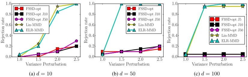
Figure 1: Rejection rates of FSSD, MMDLin and ELR-MMD on two different normal distributionsp(x) = N(x|0,Id)and q(x) =N(x|0, vId)with the variance changed in the setv ∈ {1,1.5,2,2.5}ford = 10,50,100. The abbreviation “opt” in

FSSD-opt means that all parameters in FSSD are optimized, including the kernel parameter and all test locations (Jitkrittum et al. 2017). The results of FSSD-opt for the number of test locationsJ = 5,10,50are all shown in this figure.

ity of the probabilistic models. Recently, Stein’s method (Stein and others 1972; Oates, Girolami, and Chopin 2017) has been introduced into the kernel domain (Gorham and Mackey 2017), by combining Stein’s identity with the RKHS theory, which is a likelihood-free method and de-pends onponly through logarithmic derivatives. The pro-posed statistic is referred to as kernel Stein discrepancy (KSD) (Chwialkowski, Strathmann, and Gretton 2016; Liu, Lee, and Jordan 2016). Since the null distribution of the unbiased estimator KSDUnb of KSD does not have an an-alytical form, the bootstrap was adopted to calculate the approximate rejection threshold, whose time complexity is O(n2₎_{. A linear statistic, KSD}

Lin, was proposed using half-sampling, which has a zero-mean Gaussian limit under the null hypothesis (Liu, Lee, and Jordan 2016). To improve the performance of the existing linear statistics, (Jitkrittum et al. 2017) proposed a novel statistic, the finite set Stein discrep-ancy (FSSD), by introducing a witness function on a finite set, which can conduct testing in linear time and show ex-cellent performance on low-dimensional data.

In this paper, we introduce the method of empirical likeli-hood into the domain of linear kernel tests for the first time, and propose two novel empirical likelihood ratio (ELR) statistics for the two-sample test and the goodness-of-fit test, respectively. The empirical likelihood method (Owen 1990; 2001) owes its broad usage and fast research development to a number of important advantages in statistics. Generally speaking, it combines the reliability of nonparametric meth-ods with the effectiveness of the likelihood approach. Taking into consideration the asymptotic normality of the linear un-biased estimator MMDLin(Gretton et al. 2012), we first pro-pose an ELR statistic based on the formulation of MMDLin, named ELR-MMD, for the two-sample test problem. We optimize an empirical distribution on the set of the one-dimensional pairwise discrepancies with the constraint that the empirical mean of all discrepancies is 0. We establish the nonparametric Wilks’ theorem for the statistic ELR-MMD, which shows that the proposed ELR-MMD has a limiting chi-square distribution. For the goodness-of-fit test, we pro-pose an ELR statistic based on the linear unbiased estimator

KSDLin, called ELR-KSD, by enforcing an empirical distri-bution on the pairwise discrepancies. We derive the nonpara-metric Wilks’ theorem to show the limiting distribution of ELR-KSD. The proposed ELR-MMD and ELR-KSD statis-tics show better performance than MMDLin and KSDLin, and remarkably higher discriminability (power) when test-ing two distributions with subtle differences. There are two possible reasons for the impressive performance of the ELR statistics. First, enforcing a probability on each pairwise discrepancy can help discriminate the subtle difference be-tween two distributions. Second, the rejection regions of the ELR statistics are obtained by contouring a logarithmic like-lihood ratio in what may be the most powerful test for a fixed significance levelαby Neyman-Pearson lemma (Ney-man and Pearson 1933). We further prove the consistency of the proposed ELR statistics, which guarantees that the test power (i.e., the probability of correctly rejectingH0 when H1holds) goes to 1, as the number of samples goes to infin-ity.

Another contribution of this paper is that we experimen-tally demonstrate that the recently proposed FSSD has poor performance or even fails to test for high-dimensional data. In Figure 11_{, we investigate the power of FSSD as} com-pared to MMDLin and ELR-MMD, on two normal distri-butionsp(x) = N(x|0,Id)andq(x) = N(x|0, vId)with the variance changed in the setv ∈ {1,1.5,2,2.5}ford= 10,50,100. We find that both the existing statistic MMDLin and the proposed ELR-MMD work well ford= 10,50,100, but FSSD shows poor rejection rates ford = 10, and fails to reject the null hypothesis for d = 50,100, even when the variance v is very large. We also increase an impor-tant parameter of FSSD, the number of test locations J, to further verify the performance of FSSD, but the results are almost the same (see Figure 1). We will further pro-vide a deeper understanding of FSSD and analyze the pos-sible reasons why FSSD shows poor performance on high-dimensional data. Since FSSD has shown good performance on low-dimensional data (Jitkrittum et al. 2017), the pro-posed ELR statistics can be considered as complements to

1

(3)

FSSD for high-dimensional data.

Empirical Likelihood Ratio

for Two Sample Test

In this section, we will propose an empirical likelihood ra-tio statistic for the two-sample test problem and derive its limiting distribution by Wilks’ Theorem.

Assume that the data domain is a compact setX ∈ _Rd_.

LetHκ be a reproducing kernel Hilbert space (RKHS)

de-fined onX with the reproducing kernelκ: X × X →R,

andpa Borel probability measure onX. We adopt a unit ball in a universal RKHSHκas the function classF, since

this class is rich enough to show the equivalence between the zero expectation of the statistics and the equality of two distributions (Fukumizu, Bach, and Jordan 2004; Sriperum-budur et al. 2010; Steinwart 2001; Micchelli, Xu, and Zhang 2006). Universality requires thatκis continuous andHκis

dense in the space of bounded continuous functionsC(X) with respect to theL∞norm. Gaussian and Laplace RKHSs

are universal2 (Steinwart 2001). Kernel parameters can be chosen via cross validation (Ding and Liao 2011; 2012; Liu, Jiang, and Liao 2014; Liu et al. 2018).

The mean embedding of a distributionpinF, written as µκ(p)∈ F, is defined such thatEx∼pf(x) =hf, µκ(p)ifor

allf ∈ F. The squared MMD between two distributionsp andqis the squared RKHS distance between their respective mean embeddings,

MMD2[F, p, q] =kµκ(p)−µκ(q)k2F=Ezz0h(z, z0),

wherez = (x, y),z0 = (x0, y0)andh(z, z0) = κ(x, x0) +

κ(y, y0₎₋_κ₍_{x, y}0₎₋_κ₍_x0_{, y}₎_._{It has been proved that for a}

unit ballF in a universal RKHS, MMD[F, p, q] = 0if and only ifp=q(Gretton et al. 2012).

For two sets of samplesDx={xi}ni=1⊂ X ⊆Rd, where xi∼pi.i.d., andDy ={yj}mj=1 ⊂ Y ⊆Rd, whereyi ∼q

i.i.d., if we assumem=n, the minimum variance unbiased estimator of MMD2[F, p, q]can be represented as

MMD2Unb[F,Dx,Dy] =

1

n(n−1)

n

X

i6=j

h(zi, zj).

MMDUnbrequiresO(n2)time to computehon all interact-ing pairs. The null distribution of MMDUnbdoes not have an analytical form, so the bootstrap or moment matching are re-quired withO(n2)time complexity. A linear time unbiased estimator MMDLinwas proposed in (Gretton et al. 2012),

MMD2_Lin[F,Dx,Dy] =

1

bn/2c

bn/2c X

i=1

h(z2i−1, z2i).

We will derive an empirical likelihood ratio statistic based on MMDLin. We writehi =h(z2i−1, z2i)andN =bn/2c.

When calculatinghi,i = 1, . . . , N, independent samples

are used for differenti.h1, h2, . . . , hN are i.i.d observations

2

Universal kernels can be used to approximate any target func-tion in C(X), That is, the corresponding RKHSs are dense in

C(X).

from a univariate distributionρ. We define an empirical like-lihood function as

L(ρ) =

N

Y

i=1

dρ(hi) = N

Y

i=1 pi,

wherepi =dρ(hi) = Pr(H =hi). Only distributions with

an atom of probability on eachhi have nonzero likelihood

(Owen 1988) andL(ρ)is maximized by the empirical dis-tribution functionρN(h) =N−1P

N

i=1I(hi< h), whereI

is an indicator function (Qin and Lawless 1994). The em-pirical likelihood ratio (ELR) is then defined as R(ρ) =

L(ρ)/L(ρN),and it is easy to show thatR(ρ) =QN_i₌₁N pi.

Now we define an ELR function Ψtst(µ) for the two-sample test problem in Equation (1), in which we enforce a probability {pi ≥ 0}Ni=1 on the pairwise discrepancies {hi ≥ 0}Ni=1. There are two virtues of Ψtst(µ). First, the constraintPN

i=1pihi = µforces the empirical mean to be

the expectationµ, which makes the maximum of the empir-ical likelihood ratio more trustful. For example, in the two-sample test, underH0 :p=q, we haveE[hi] = 0and the

constraintPN

i=1pihi= 0guarantees the empirical mean of

all discrepancieshito be 0. Second, optimizing the

probabil-itypion each pairwise discrepancyhican help discriminate

the subtle difference between two distributions.

Ψtst(µ)

= max

{pi≥0}Ni=1

(N

Y

i=1 N pi

N

X

i=1 pi= 1,

N

X

i=1

pihi=µ

)

. (1)

A unique value for the right-hand side of Equation (1) exists, provided thatµis inside the convex hull of the points h1, . . . , hN (Owen 1990; 2001). An explicit expression for

Ψtst(0)can be derived by a Lagrange multiplier argument: the maximum ofQN

i=1N pisubject to the constraintspi≥0,

PN

i=1pi= 1andP N

i=1pihi= 0is attained when

pi=

1

N

1

1 +λhi

,

whereλis the solution toPN

i=1

hi

1+λhi = 0.

Now we propose an ELR test statistic for the two-sample test problem as

Wtst(0) =−2 log Ψtst(0) = 2

N

X

i=1

log(1 +λhi).

We derive the Wilks’ theorem (Theorem 1) for the ELR test statisticWtst(0), which shows thatWtst(0)has a limit-ing chi-square distribution.

Theorem 1 (Wilks’ Theorem). Under H0 : p = q, if

Ex,x0[κ2(x, x0)]<∞, the ELR test statistic

Wtst(0)

d

−→χ2₍₁₎,

where χ2

(4)

Based on Theorem 1, we can conduct two-sample test in this way: we will reject the null hypothesis H0, when Wtst(0)≥χ2α, whereχ2αis defined such that

Pr(χ2₍₁₎≥χ2_α) =α.

Since the limiting distribution isχ2

(1), we can obtain the threshold for rejection directly from the chi-square table, without needing time-consuming bootstraps or simulations. The main computational burden forWtst(0)is the calcula-tion ofhi,i = 1, . . . , N. Therefore, the time complexity of

Wtst(0)is linear in the number of samples. The proposed ELR statistic can easily be extended to B-test (Zaremba, Gretton, and Blaschko 2013), since the statistics for different blocks in B-test are independent from each other.

Theorem 2 guarantees the test consistency of the proposed ELR statistic Wtst(0), that is, when the number of sam-ples are large enough, Wtst(0)can always correctly reject the null hypothesis. We write PrH1 for the distribution of Wtst(0)underH1.

Theorem 2. UnderH1 : p6= q, ifEx,x0[κ2(x, x0)] <∞,

the test power,

Pr

H1

Wtst(0)≥χ2α

→1,

asn→ ∞.

Empirical Likelihood Ratio

for Goodness of Fit Test

In this section, we will propose an ELR statistic for the goodness-of-fit test problem and derive its limiting distri-bution by Wilks’ Theorem.

We first introduce the Stein operator (Stein and others 1972; Oates, Girolami, and Chopin 2017), which depends on the distributionponly through logarithmic derivatives. A Stein operator Tp takes a multivariate function f(x) =

(f1(x), . . . , fd(x))T ∈ Rd as input and outputs a function

(Tpf)(x) :Rd→R.The functionTpf has the key property

that for allfs in an appropriate function class,

Ex∼q[(Tpf)(x)] = 0

if and only ifp =q. Thus, this expectation can be used to test the goodness-of-fit: how well a model density pfits a set of given samplesDx = {xi}ni=1 ⊂ X ⊆ Rd from an unknown distributionq.

We consider the function classFd_:=_{F × · · · × F}_{, where}

Fis a unit-norm ball in a universal RKHS. Assume thatfi∈

Ffor alli= 1, . . . dso thatf ∈ Fd_{with the inner product}

hf, f0i_Fd :=Pd_i₌₁hfi, fi0iF.According to the reproducing

property ofF, fi(x) = hfi, κ(x,·)iF, and that ∂κ∂x(x,i·) ∈

F, we can defineωp(x,·) =

∂logp(x)

∂x κ(x,·) + κ(x,·)

∂x .The

kernel Stein operator can be written as

(Tpf)(x) =

d

X

i=1

_∂_log_p₍_x₎

∂xi

fi(x) +

∂fi(x)

∂xi

=hf, ωp(x,·)iFd.

Kernel Stein discrepancy (KSD) is defined as

KSD[Fd,Dx, p] = sup

kfk_Fd≤1

hf,Ex∼qωp(x,·)i

:=kg(·)kFd,

(2)

where g(·) = Ex∼qωp(x,·). When Ex∼pk∇xlogp(x)−

∇xlogq(x)k<∞, it can be shown that KSD[Fd,Dx, p] =

0if and only ifp=q. The squared KSD can be written as

KSD2[Fd_,_D

x, p] =Ex∼qEx0_∼_qh_p(x, x0),

wherehp(x, x0) =sTp(x)sp(x0)κ(x, x0) +sTp∇xκ(x, x0) +

sT_p∇x0κ(x, x0) +Pd_i₌₁ ∂ 2_κ₍_x,x0₎

∂xi∂x0i , and sp(x) = ∇xlogp,

which is called the score function. We denote the unbiased empirical estimator of KSD (Liu, Lee, and Jordan 2016) as

KSD2_Unb[Fd_,_D x, p] =

2

n(n−1) X

i<j

hp(xi, xj).

The computational cost of KSD2UnbisO(n2). To reduce this cost, a linear time estimator was proposed in (Liu, Lee, and Jordan 2016) and we write it as

KSD2Lin[F

d

,Dx, p] =

1

bn/2c

bn/2c X

i=1

hp(x2i−1, x2i).

Now we derive an ELR statistic for the goodness-of-fit test problem. We write hp,i = hp(x2i−1, x2i) and

N = bn/2c. When calculating hp,i, i = 1, . . . , N,

different independent samples are used for different i. hp,1, hp,2, . . . , hp,N are i.i.d observations from a univariate

distribution. Now we define an ELR function

Ψgoft(µ)

= sup

{pi≥0}Ni=1

(N

Y

i=1 N pi

N

X

i=1 pi= 1,

N

X

i=1

pihp,i=µ

)

.

Under H0 : p = q, we have E[hp,i] = 0and set µ = 0.

We use the Lagrange multiplier method to derive the explicit expression ofΨgoft(0). Fori= 1, . . . , N, we have

pi=

1

N

1

1 +λhp,i

,

whereλis the solution toPN

i=1

hp,i

1+λhp,i = 0.

Now we define an ELR test statistic for the goodness of test problem as follows,

Wgoft(0) =−2 log Ψgoft(0) = 2

N

X

i=1

log (1 +λhp,i).

We derive the Wilks’ theorem forWgoft(0), which shows a limiting chi-square distribution ofWgoft(0).

Theorem 3 (Wilks’ Theorem). Under H0 : p = q, if

Ex,x0[κ2(x, x0)]<∞, the ELR test statistic

Wgoft(0)

d

−

(5)

Based on Theorem 3, we will rejectH0, whenWgoft(0)≥ χ2αwithχ2αsatisfyingPr(χ2(1) ≥χ

2

α) =α.The main

com-putational burden for Wgoft(0) is the calculation of hp,i,

i = 1, . . . , N. Therefore, the time complexity ofWgoft(0) is linear in the number of samples.

Theorem 4 guarantees the test consistency ofWgoft(0).

Theorem 4. UnderH1 : p6= q, ifEx,x0[κ2(x, x0)] <∞,

the test power,

Pr

H1

Wgoft(0)≥χ2α

→1,

asn→ ∞.

Comparisons with FSSD

In this section, we compare FSSD (Jitkrittum et al. 2017) with existing linear statistics and our ELR statistics, and an-alyze the possible reasons why FSSD shows poor perfor-mance or even fails for high-dimensional data.

We first briefly introduce FSSD. LetV ={v1, . . . , vJ} ⊂ Rdbe random vectors drawn from a distribution. The

statis-tic of FSSD is defined as

FSSD2_p(q) = 1

dJ

d

X

i=1

J

X

j=1 g2_i(vj),

whereg(·)is referred to as the Stein witness function, given in Equation (2). It has been proved (Jitkrittum et al. 2017) that if the following conditions are satisfied, 1)κis a uni-versal and analytic function; 2) Ex∼qEx0_∼_ph_p(x, x0) <

∞; 3) Ex∼qk∇xlogp(x)− ∇xlogq(x)k2 < ∞; and 4)

lim_kxk→∞p(x)g(x) = 0; for any J ≥ 1, almost surely

FSSD2p(q) = 0if and only ifp=q. LetΩ(x)∈Rd×Jsuch

that [Ω(x)]i,j = ωp,i(x, vj)/

√

dJ , τ(x) = vec(Ω(x)) ∈

RdJ, wherevec(·)denotes the vectorization, and∆(x, y) = τ(x)T_τ₍_y₎_{. The unbiased estimator of FSSD}2

p(q)is

\

FSSD2= 2

n(n−1) X

i<j

∆(xi, xj).

In the following, we explain why FSSD is different from MMDLin, KSDLin, ELR-MMD and ELR-KSD and why FSSD shows poor performance on high-dimensional data.

For MMDLin, KSDLin, ELR-MMD and ELR-KSD, one data pointxionly corresponds to a one-dimensional

statisti-cal value, such ashiorhp,i, but for\FSSD

2

, one data pointxi

corresponds to ad×JmatrixΩ(x)or adJ-dimensional vec-torτ(x). The underlying reason for the higher dimensional correspondence of FSSD is the introduction of the finite set. The finite set makes the kernel function κ(x,·) no longer only appear in the dot product form with another function f ∈ F, which is different from the forms in MMDLin, KSDLin, ELR-MMD and ELR-KSD. In a word, this makes FSSD more closely related to the dimensiondof data than other linear statistics. In addition, the higher dimensional correspondence makes the empirical likelihood difficult to be applied in FSSD. The elements inτ(x)for FSSD are not independent, so if we enforce a probability distribution on

the set ofτ(xi),i= 1, . . . , n, the empirical likelihood ratio

does not have a limitingχ2

dJ distribution.

According to Proposition 2 in (Jitkrittum et al. 2017), un-der theH1:p6=q,

nFSSD\2∼√nN(0, σH1) +nFSSD

2 ,

if σH1 = 4µ

T_Σq_{µ >} ₀_{, where} _µ ₌ _Ex

∼q[τ(x)] and

Σq = covx∼q[τ(x)] ∈ RdJ×dJ. From the above

equa-tion, we know thatn\FSSD2is highly dependent on the di-mension of the data: when the didi-mensiond increases, the dimension ofΣq will increase, and then the varianceσH1

becomes larger. When the variance becomes larger, the re-sulting values of the statistic will become unstable. For MMDLin, KSDLin, ELR-MMD and ELR-KSD, the kernel functionκ(x,·)only appears in the dot product form, and thus the statistics are less dependent on the dimensiondof data.

In addition, underH0 : p = q, the asymptotic

distribu-tion ofnFSSD\

2

is not an analytical form, but the existing linear statistics MMDLin and KSDLin, and the ELR statis-tics ELR-MMD and ELR-KSD all have analytical limiting distributions.

Experiments

Here we conduct a series of experiments to evaluate the per-formance of the proposed ELR statistics and exploit the con-ditions under which the proposed statistics can perform well. We compare the ELR statistics, MMD and ELR-KSD, with three existing linear nonparametric statistics, in-cluding MMDLin(Lin-MMD) (Gretton et al. 2012), KSDLin (Lin-KSD) (Liu, Lee, and Jordan 2016) and FSSD (FSSD-opt)3 (Jitkrittum et al. 2017). Because Gaussian kernels are universal (Steinwart 2001), we adopt Gaussian kernels

κ(x, x0) = exp −γkx−x0k2

2

with variable width γ ∈ {2−10_,₂−9_{, . . . ,}₂10_} _{as our candidate kernel set. For all} evaluations, we set the significance levelα= 0.05. All ex-periments are repeated 100 times. All implementations are in Python and R.

We investigate the power of Lin-MMD, Lin-KSD, ELR-MMD, ELR-KSD and FSSD, and provide deep insights into the proposed statistics.

The first set of experiments are conducted on two Gaus-sians p(x) = N(x|0,Id)and q(x) = N(x|0, vId), with

variable variancev ∈ {1.1,1.3, . . . ,2.3}. We adopt a fixed dimensiond= 100. To investigate the influence of the num-ber of samples on the gap between the ELR statistics (ELR-MMD and ELR-KSD) and the existing linear statistics (Lin-MMD and Lin-KSD), we observe the rejection rates of the statistics for different numbers of samples. The results are shown in Figure 2. We can find that the gap between Lin-MMD and ELR-Lin-MMD or between Lin-KSD and ELR-KSD becomes smaller as the number of samples becomes larger.

3

(6)

1.1 1.3 1.5 1.7 1.9 2.1 2.3 Variance Perturbation 0.0 0.2 0.4 0.6 0.8 1.0 Rejection rate FSSD-opt Lin-MMD ELR-MMD

(a)n= 40

(b)n= 200

(c)n= 400

1.1 1.3 1.5 1.7 1.9 2.1 2.3 Variance Perturbation 0.1 0.2 0.3 0.4 0.5 0.6 0.7 0.8 0.9 1.0 Rejection rate FSSD-opt Lin-MMD ELR-MMD

(d)n= 800

1.1 1.3 1.5 1.7 1.9 2.1 2.3 Variance Perturbation 0.00 0.05 0.10 0.15 0.20 0.25 Rejection rate FSSD-opt Lin-KSD ELR-KSD

(a)n= 200

1.1 1.3 1.5 1.7 1.9 2.1 2.3 Variance Perturbation 0.0 0.1 0.2 0.3 0.4 0.5 Rejection rate FSSD-opt Lin-KSD ELR-KSD

(b)n= 400

1.1 1.3 1.5 1.7 1.9 2.1 2.3 Variance Perturbation 0.0 0.1 0.2 0.3 0.4 0.5 0.6 Rejection rate FSSD-opt Lin-KSD ELR-KSD

(c)n= 800

1.1 1.3 1.5 1.7 1.9 2.1 2.3 Variance Perturbation 0.0 0.1 0.2 0.3 0.4 0.5 0.6 0.7 0.8 0.9 Rejection rate FSSD-opt Lin-KSD ELR-KSD

(d)n= 1000

Figure 2: Rejection rates of Lin-MMD, ELR-MMD, Lin-KSD, ELR-KSD and FSSD on two different normal distributions p(x) =N(x|0,Id)andq(x) =N(x|0, vId)with the variance changed in the setv∈ {1.1,1.3, . . . ,2.3}ford= 100.

10 40 70 100

Dimension 0.0 0.1 0.2 0.3 0.4 0.5 0.6 0.7 0.8 Rejection rate FSSD-opt Lin-MMD ELR-MMD

(a)n= 80

10 40 70 100

Dimension 0.0 0.1 0.2 0.3 0.4 0.5 0.6 0.7 Rejection rate FSSD-opt Lin-MMD ELR-MMD

(b)n= 400

10 40 70 100

Dimension 0.0 0.1 0.2 0.3 0.4 0.5 0.6 Rejection rate FSSD-opt Lin-MMD ELR-MMD

(c)n= 2000

10 40 70 100

Dimension 0.0 0.2 0.4 0.6 0.8 1.0 Rejection rate FSSD-opt Lin-MMD ELR-MMD

(d)n= 10000

10 40 70 100

Dimension 0.0 0.2 0.4 0.6 0.8 1.0 Rejection rate FSSD-opt Lin-KSD ELR-KSD

(a)n= 80

10 40 70 100

(b)n= 400

10 40 70 100

(c)n= 2000

10 40 70 100

Dimension 0.0 0.2 0.4 0.6 0.8 1.0 Rejection rate _FSSD-opt Lin-KSD ELR-KSD

(d)n= 10000

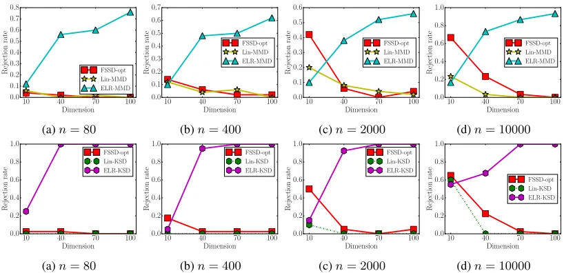
Figure 3: Rejection rates of Lin-MMD, ELR-MMD, Lin-KSD, ELR-KSD and FSSD on Gaussianp(x) = N(x|0,Id)and

Laplacianq(x) =Qd

i=1Laplace(xi|0,1/

√

2)with variable dimensiond∈ {10,40,70,100}forn= 80,400,2000,10000.

The possible reason is that, under H0 : p = q, the influ-ence of the enforced constraintPN

i=1pihi= 0will become

smaller as number of samples increases, since the expecta-tion of the discrepancyhi is 0. We can also see that the

re-jection rates of Lin-MMD and ELR-MMD are higher than those of Lin-KSD and ELR-KSD. In this experiment, FSSD shows low rejection rates or fails to test nearly in all cases, while the existing linear statistics Lin-MMD and Lin-KSD and the proposed statistics ELR-MMD and ELR-KSD can perform normally. These results are in agreement with the analyses given in the last section.

In the second experiment, we adopt the distributions Gaussian p(x) = N(x|0,Id) and Laplacian q(x) =

Qd

i=1Laplace(xi|0,1/

√

(7)

1000 4000 7000 10000 13000 Sample Size

0 10 20 30 40 50 60 70

Time

(s)

FSSD-opt Lin-KSD ELR-KSD Lin-MMD ELR-MMD

Figure 4: Running time of FSSD, Lin-MMD, ELR-MMD, Lin-KSD and ELR-KSD on Gaussianp(x) = N(x|0,Id) and Laplacianq(x) =Qd

i=1Laplace(xi|0,1/

√

2)withd=

100with variable sizen∈ {1000,2000, . . . ,14000}.

in this experiment even with a large sample size, whereas ELR-MMD and ELR-KSD show remarkably good mance. There are two reasons for the impressive perfor-mance of the ELR statistics. First, enforcing a probabil-ity on each pairwise discrepancy can help discriminate the subtle difference between two distributions. Second, the re-jection thresholds of the ELR statistics are determined by contouring a logarithmic likelihood ratio, which may be the most powerful test for a fixedα. This point still needs to be theoretically supported by proving the empirical version of the Neyman-Pearson lemma (Neyman and Pearson 1933). It is known that FSSD has shown good performance on low-dimensional data (Jitkrittum et al. 2017). The proposed ELR statistics can be considered as complements to FSSD for high-dimensional data, since they have shown higher power than the existing linear statistics.

In the third experiment, we compare the running time of all linear statistics. The results are shown in Figure 4. We observe that the running time of the ELR statistics ELR-MMD and ELR-KSD are almost the same as that of the lin-ear statistics Lin-MMD and Lin-KSD, and all these linlin-ear statistics are much faster than FSSD. There are two reasons for the low efficiency of FSSD. First, under the null hypoth-esis, the asymptotic distribution of FSSD is not an analytical form, so it requires bootstraps or simulations to calculate the threshold for rejecting the null hypothesis (Jitkrittum et al. 2017), which is time-consuming. Second, FSSD optimizes the test locationsV ={v1, . . . , vJ} ⊂Rdvia gradient

as-cent to get better performance than FSSD-rand4_(Jitkrittum et al. 2017).

In the fourth experiment, we check the Type I errors (false rejection rates) of all linear statistics. We consider a 10-dimensional Gaussian distribution and a Gaussian-Bernoulli restricted Boltzmann machine (RBM) (Liu, Lee, and Jordan 2016), which is a hidden variable graphical model consist-ing of a continuous observable variablex∈Rdand a binary

hidden variabler∈ {±1}dh_{, with joint probability}

p(x, r) = 1

Zexp(x

T_Br₊_bT_x₊_cT_x

−1

2kxk

2₎_.

4

In FSSD-rand, the test locations are set to random draws from a multivariate normal distribution (Jitkrittum et al. 2017).

1000 2000 3000 4000 Sample sizen

0.03 0.04 0.05 0.06 0.07 0.08 0.09

Rejection

rate

1000 2000 3000 4000 Sample sizen

0.02 0.03 0.04 0.05 0.06 0.07

Rejection

rate

Figure 5: Type I errors (false rejection rates) of all linear tests with variable sizen ∈ {1000,2000,3000,4000}. The first one is for the 10-dimensional Gaussian distribution and the second one is for RBM.

The results are shown in Figure 5, which shows the rejection rates of all the tests as the sample size increases whenpand qare the same Gaussian or RBM distribution. We find that all the tests have roughly the right false rejection rates at the set significance levelα= 0.05

Conclusions

In this paper, we established the first connection between the empirical likelihood and nonparametric kernel tests, and derived novel empirical likelihood ratio (ELR) statistics for the two-sample test and the goodness-of-fit test. We pro-vided theoretical insights indicating that the ERL statistics have limiting chi-square distributions under the null hypoth-esis, and that their test consistencies hold under the alter-native hypothesis. The new ELR statistics have empirically shown stronger test power than the existing linear statistics for high-dimensional data while preserving high computa-tional efficiency. In the near future, we will develop ELR statistics for other nonparametric statistical test problems, including the independence test and the conditional indepen-dence test.

Acknowledgments

(8)

References

Chwialkowski, K.; Strathmann, H.; and Gretton, A. 2016. A kernel test of goodness of fit. InICML, 2606–2615.

Cucker, F., and Smale, S. 2002. On the mathematical founda-tions of learning. Bulletin of the American Mathematical Society

39(1):1–49.

Ding, L., and Liao, S. 2011. Approximate model selection for large scale LSSVM. Journal of Machine Learning Research - Proceed-ings Track20:165–180.

Ding, L., and Liao, S. 2012. Nystr¨om approximate model selection for LSSVM. InAdvances in Knowledge Discovery and Data Min-ing — ProceedMin-ings of the 16th Pacific-Asia Conference (PAKDD), 282–293.

Ding, L., and Liao, S. 2014a. Approximate consistency: Towards foundations of approximate kernel selection. InProceedings of the European Conference on Machine Learning and Principles and

Practice of Knowledge Discovery in Database (ECML PKDD),

354–369.

Ding, L., and Liao, S. 2014b. Model selection with the covering number of the ball of RKHS. InProceedings of the 23rd ACM International Conference on Information and Knowledge Manage-ment (CIKM), 1159–1168.

Ding, L., and Liao, S. 2017. An approximate approach to automatic kernel selection. IEEE Transactions on Cybernetics47(3):554– 565.

Ding, L.; Liao, S.; Liu, Y.; Yang, P.; and Gao, X. 2018. Random-ized kernel selection with spectra of multilevel circulant matrices. InProceedings of the 32nd AAAI Conference on Artificial Intelli-gence (AAAI), 2910–2917.

Ding, L.; Liu, Y.; Liao, S.; Li, Y.; Yang, P.; Pan, Y.; Huang, C.; Shao, L.; and Gao, X. 2019. Approximate kernel selection with strong approximate consistency. InProceedings of the 33rd AAAI Conference on Artificial Intelligence (AAAI).

Fukumizu, K.; Bach, F. R.; and Jordan, M. I. 2004. Dimensionality reduction for supervised learning with reproducing kernel Hilbert spaces.Journal of Machine Learning Research5:73–99.

Gorham, J., and Mackey, L. 2017. Measuring sample quality with kernels. InICML, 1292–1301.

Gretton, A.; Borgwardt, K. M.; Rasch, M. J.; Sch¨olkopf, B.; and Smola, A. J. 2012. A kernel two-sample test. Journal of Machine Learning Research13:723–773.

Jitkrittum, W.; Xu, W.; Szab´o, Z.; Fukumizu, K.; and Gretton, A. 2017. A linear-time kernel goodness-of-fit test. InNIPS 30, 261– 270.

Li, C.-L.; Chang, W.-C.; Cheng, Y.; Yang, Y.; and P´oczos, B. 2017. MMD GAN: Towards deeper understanding of moment matching network. InNIPS 30, 2203–2213.

Li, J.; Liu, Y.; Yin, R.; Zhang, H.; Ding, L.; and Wang, W. 2018. Multi-class learning: from theory to algorithm. InNeurIPS 31, 1593–1602.

Liu, Y., and Liao, S. 2015. Eigenvalues ratio for kernel selection of kernel methods. InAAAI, 2814–2820.

Liu, Y.; Liao, S.; Lin, H.; Yue, Y.; and Wang, W. 2017. Infinite kernel learning: generalization bounds and algorithms. InAAAI, 2280–2286.

Liu, Y.; Lin, H.; Ding, L.; Wang, W.; and Liao, S. 2018. Fast cross-validation. InIJCAI, 2497–2503.

Liu, Y.; Jiang, S.; and Liao, S. 2014. Efficient approximation of cross-validation for kernel methods using Bouligand influence function. InICML, 324–332.

Liu, Q.; Lee, J.; and Jordan, M. 2016. A kernelized Stein discrep-ancy for goodness-of-fit tests. InICML, 276–284.

Lloyd, J. R., and Ghahramani, Z. 2015. Statistical model criticism using kernel two sample tests. InNIPS 28, 829–837.

Micchelli, C. A.; Xu, Y.; and Zhang, H. 2006. Universal kernels.

Journal of Machine Learning Research7:2651–2667.

Muandet, K.; Fukumizu, K.; Sriperumbudur, B.; Sch¨olkopf, B.; et al. 2017. Kernel mean embedding of distributions: A review and beyond. Foundations and Trends in Machine Learning 10(1-2):1–141.

Neyman, J., and Pearson, E. S. 1933. On the problem of the most efficient tests of statistical inference.Biometrika A20:175–240. Oates, C. J.; Girolami, M.; and Chopin, N. 2017. Control function-als for Monte Carlo integration. Journal of the Royal Statistical Society: Series B (Statistical Methodology)79(3):695–718. Owen, A. B. 1988. Empirical likelihood ratio confidence intervals for a single functional.Biometrika75(2):237–249.

Owen, A. B. 1990. Empirical likelihood ratio confidence regionsn.

Annals of Statistics18(1):90–120.

Owen, A. B. 2001.Empirical Likelihood. Chapman and Hall/CRC, New York.

Qin, J., and Lawless, J. 1994. Empirical likelihood and general estimating equations.Annals of Statistics300–325.

Song, L.; Smola, A. J.; Gretton, A.; Bedo, J.; and Borgwardt, K. 2012. Feature selection via dependence maximization. Journal of Machine Learning Research13:1393–1434.

Sriperumbudur, B. K.; Fukumizu, K.; Gretton, A.; Lanckriet, G. R.; and Sch¨olkopf, B. 2009. Kernel choice and classifiability for RKHS embeddings of probability distributions. InNIPS 22, 1750– 1758.

Sriperumbudur, B. K.; Gretton, A.; Fukumizu, K.; Sch¨olkopf, B.; and Lanckriet, G. R. G. 2010. Hilbert space embeddings and met-rics on probability measures. Journal of Machine Learning Re-search11:1517–1561.

Stein, C., et al. 1972. A bound for the error in the normal approxi-mation to the distribution of a sum of dependent random variables. InProceedings of the 6th Berkeley Symposium on Mathematical Statistics and Probability, Volume 2: Probability Theory.

Steinwart, I. 2001. On the influence of the kernel on the consis-tency of support vector machines. Journal of Machine Learning Research2:67–93.

Yang, P.; Zhao, P.; Zheng, V. W.; Ding, L.; and Gao, X. 2018. Robust asymmetric recommendation via min-max optimization. In

SIGIR, 1077–1080.