Random Feature Maps for the Itemset Kernel

(1)

The Thirty-Third AAAI Conference on Artificial Intelligence (AAAI-19)

Random Feature Maps for the Itemset Kernel

Kyohei Atarashi

Hokkaido University

atarashi [email protected]

Subhransu Maji

University of Massachusetts, Amherst [email protected]

Satoshi Oyama

Hokkaido University/RIKEN AIP

[email protected]

Abstract

Although kernel methods efficiently use feature combinations without computing them directly, they do not scale well with the size of the training dataset. Factorization machines (FMs) and related models, on the other hand, enable feature com-binations efficiently, but their optimization generally requires solving a non-convex problem. We present random feature maps for the itemset kernel, which uses feature combina-tions, and includes the ANOVA kernel, the all-subsets ker-nel, and the standard dot product. Linear models using one of our proposed maps can be used as an alternative to kernel methods and FMs, resulting in better scalability during both training and evaluation. We also present theoretical results for a proposed map, discuss the relationship between factoriza-tion machines and linear models using a proposed map for the ANOVA kernel, and relate the proposed feature maps to prior work. Furthermore, we show that the maps can be calculated more efficiently by using a signed circulant matrix projection technique. Finally, we demonstrate the effectiveness of using the proposed maps for real-world datasets.

1 Introduction

Kernel methods enable learning in high, possibly infinite dimensional feature spaces without explicitly expressing them. In particular, kernels that model feature combina-tions such as polynomial kernels, the ANOVA kernel, and the all-subsets kernel (Blondel et al. 2016a; Shawe-Taylor and Cristianini 2004) have been shown to be effective for a number of tasks in computer vision and natural lan-guage understanding (Lin, RoyChowdhury, and Maji 2015; Fukui et al. 2016). However their scalability remains a chal-lenge; support vector machines (SVMs) with non-linear ker-nels requireO(n2₎_{time and}_O₍_n2₎_{memory for training and} O(n)time and memory for evaluation, wherenis the num-ber of training instances (Chang and Lin 2011).

To address this issue several researchers have proposed randomized feature maps Z(·) : Rd 7→ RD for kernels

K(·,·) :_Rd_×

Rd7→Rthat satisfy

E[hZ(x), Z(y)i] =K(x,y). (1)

The idea is to perform classification, regression, or cluster-ing on a correspondcluster-ing high-dimensional feature space

proximately but efficiently using linear models in a low di-mensional space by mapping the data points usingZ(·). Ex-amples includerandom Fourier feature mapsthat approxi-mate shift-invariant kernels:K(x,y) =k(|x−y|)(Rahimi and Recht 2008);random Maclaurin feature mapsthat ap-proximate dot product kernels (Kar and Karnick 2012): K(x,y) =k(hx,yi); andtensor sketchingfor polynomial kernels: K_Pm(x,y;c) := (c +hx,yi)m (Pham and Pagh 2013). Although polynomial kernels are dot product ker-nels and can be approximated by random Maclaurin feature maps, tensor sketching can be more efficient.

Factorization machines (FMs) (Rendle 2010; 2012) and variants (Blondel et al. 2016a; 2016b; Novikov, Trofimov, and Oseledets 2016) also model feature combinations with-out explicitly computing them, similar to kernel methods, but have better scalability during evaluation. These meth-ods can be thought of as a two-layer neural network with polynomial activations with a fixed number of learnable pa-rameters (See Equation (5)). However, unlike kernel meth-ods, their optimization problem is generally non-convex and difficult to solve. But due to their efficiency during evalu-ation FMs are attractive for large-scale problems and have been successfully applied to applications such as link pre-diction and recommender systems. This work analyzes the relationship between polynomial kernel models and factor-ization machines in more detail.

(2)

2 Background and Related Work

2.1 Kernels Using Feature Combinations

First, we present the ANOVA kernel and all-subsets ker-nel, which use feature combinations (Blondel et al. 2016a; Shawe-Taylor and Cristianini 2004), and define the item-set kernel. We also describe several models that use feature combinations.

The ANOVA kernel is similar to the polynomial kernel. The definition of anm-order ANOVA kernel betweenx,y∈

Rdis

KAm(x,y) :=

d X

j1<···<jm

xj1· · ·xjmyj1· · ·yjm, (2)

where2 ≤ m ≤ d ∈ _Nis the order of the ANOVA ker-nel. For convenience,0/1-order ANOVA kernels are often defined as K0

A(x,y) = 1 and KA1(x,y) = hx,yi. The difference between the ANOVA kernel and the polynomial kernel is that the ANOVA kernel does not use feature com-binations that include the same feature (e.g., x1x1, x22x3) while the polynomial kernel does. Although the evaluation of the m-order ANOVA kernel involves O(dm₎ _{terms, it}

can be computed inO(dm)time using dynamic program-ming (Blondel et al. 2016a; Shawe-Taylor and Cristianini 2004). In some applications, ANOVA-kernel-based models have achieved better performance than polynomial-kernel-based models (Blondel et al. 2016a; 2016b). We discuss these models later in this section.

While the ANOVA kernel uses onlym-order different fea-ture combinations, the all-subsets kernelKalluses all differ-ent feature combinations and is defined as

Kall(x,y) :=

d Y

j=1

(1 +xjyj). (3)

Clearly, evaluation of the all-subsets kernel takes onlyO(d)

time.

Here, we define the itemset kernel. For a given family of itemsetsS ⊆ 2[d], where[d] = {1, . . . , d} and2[d] =

{∅,{1},{2}, . . . ,{d},{1,2}, . . . ,[d]}, we define the item-set kernel as

KS(x,y) := X

V∈S Y

j∈V

xjyj =hφS(x), φS(y)i. (4)

The itemset kernel clearly uses feature combinations in the family of itemsetsS. The itemset kernel can be regarded as an extension of the ANOVA kernel, all-subsets kernel, and standard dot product. For example, whenS = 2[d],K2[d] clearly uses all feature combinations and hence is equivalent to the all-subsets kernelKall in Equation (3). WhenS =

[d]

m

:= {V ⊆ [d] | |V| = m}, the itemset kernelKS

is equivalent tom-order ANOVA kernelKm

A. Furthermore, when S = {{1}, . . . ,{d}}, the itemset kernelKS clearly

represents the standard dot product.

2.2 Factorization Machines

Rendle proposed using afactorization machine (FM)as the ANOVA-kernel-based model (Rendle 2010; 2012). The FM

model equation is

fFM(x;w,P,λ) :=hw,xi+

k X

s=1

λsKA2(ps,x), (5)

wherew ∈ Rd,P ∈ Pd×k, andλ∈ Rk are learnable

pa-rameters, andk ∈ _Nis a rank-hyper parameter. The com-putational cost for evaluating FMs is O(dkm) and does not depend on the amount of training data. However, the FM optimization problem is non-convex and hence chal-lenging. Fortunately, it can be solved relatively efficiently using a coordinate descent method because it is multi-convex w.r.t w1, . . . , wd, p1,1, . . . , pd,k. Although

parame-terλwas not introduced in the original FMs (Rendle 2010; 2012), Blondel et al. showed that introducingλincreases the capacity of FMs (Blondel et al. 2016b).

Polynomial networks (PNs) (Livni, Shalev-Shwartz, and Shamir 2014) are models based on polynomial kernels. They are depth two neural networks with a polynomial activation function. Although both PNs and FMs use feature combina-tions, there is a key difference: PNs can be represented by the polynomial kernel while FMs can be represented by the ANOVA kernel. This difference means PNs use feature com-binations among the same features while FMs do not. Ex-periments have shown that FMs achieve better performance than PNs (Blondel et al. 2016a).

Blondel et al. proposed theall-subsets model(Blondel et al. 2016a), which uses all feature combinations:

fall(x;P,λ) :=

k X

s=1

λsKall(ps,x). (6)

Although the all-subsets model sometimes performed better than FMs and PNs on link prediction tasks, it tended to have lower performance (Blondel et al. 2016a).

2.3 Random Feature Maps for Polynomial

Kernels

The random Maclaurin (RM) feature map (Kar and Karnick 2012) is for dot product kernels: K(x,y) = k(hx,yi). It uses the Maclaurin expansion ofk(·):k(x) =P∞

n=0anx

n_,

where an = k(n)(0)/n! is the n-th coefficient of the

Maclaurin series. It uses two distributions: porder(N =

n) = 1/pn+1_{, where}_{p >} ₁_{, and the Rademacher} distri-bution (a fair coin distridistri-bution). Its computational cost is O PD

s=1Nsd

time and memory, whereNs(s∈[D]) is the

order of the s-th randomized feature, especially O(Ddm)

time and memory when the objective kernel is the homoge-neous polynomial kernel:Km

HP(x,y) =hx,yim.1

The tensor sketching (TS) (Pham and Pagh 2013) is a random feature map for homogeneous polynomial ker-nels :K_HPm(x,y) = hx,yim_{. Because polynomial kernels}

Km

P(x,y;c) = (c+hx,yi)m can be written asKHPm by concatenating√cto each vector, a TS can approximateKm

P. 1

When the objective kernel is a homogeneous polynomial ker-nel, one can fixn=mandporder(N=m) = 1otherwise0; that

(3)

Algorithm 1Random Kernel Feature Map

Input: x∈_Rd_,_{S ⊆}₂[d]

1: Generate D Rademacher vectors ω1, . . . ,ωD ∈ {−1,+1}d

2: ComputeDitemset kernelsKS(x,ωs)for alls∈[D]

Output: Z(x) =√1

D KS(x,ω1), . . . , KS(x,ωD) >

Although an RM feature map can also approximate polyno-mial kernels, a TS can approximate them more efficiently. It uses the count sketch method, which is a method for esti-mating the frequency of all items in a stream, as a specific random projection that approximates the dot product in the original feature space. Although the standard dot product in the original feature space can be approximated by using only count sketch, Pham and Pagh proposed combining count sketch with a fast algorithm for computing the count sketch of the outer product without computing the outer product directly, which was proposed by Pagh (Pagh 2013). Their tensor sketch algorithm takesO(m(d+DlogD))time and O(mdlogD)memory and is thus more efficient than the random Maclaurin algorithm.

Linear models using the TS or RM feature map are a good alternative to polynomial kernel SVMs and PNs (Kar and Karnick 2012; Pham and Pagh 2013). Similarity, although linear models using a random feature map that approxi-mates the itemset kernel would be a good alternative for the ANOVA or all-subsets kernel SVMs, FMs, and all-subsets models, such a map has not yet been reported.

3 Random Feature Map for the Itemset

Kernel

We propose a random feature map for the itemset kernel. As shown in Algorithm 1, the proposedrandom kernel (RK) mapis simple: (1) generateD Rademacher vectors from a Rademacher distribution and (2) computeDitemset kernels between the original feature vector and each Rademacher vector. We next present some theoretical results for the RK feature map.

Proposition 1. LetZRK:Rd7→RDbe the random kernel

(RK) feature map in Algorithm 1. Then, for allx,y ∈ Rd

andS ⊆2[d]_,

Eω1,...,ωD[hZRK(x), ZRK(y)i] =KS(x,y). (7)

Proposition 1 says that the proposed RK feature map ap-proximates the itemset kernel. Hence, linear models using the proposed RK feature map can use feature combinations efficiently and are a good alternative to FMs and all-subsets models.

We next analyze the precision of the RK feature map. Let E(x,y) be the approximation error: E(x,y) :=

hZRK(x), ZRK(y)i − KS(x,y). We assume that the L1

norm of the feature vector is bounded: kxk1 ≤ R, where R ∈ _R++. This assumption is the same as the one used in previous research (Kar and Karnick 2012; Pham and Pagh

2013; Rahimi and Recht 2008). For convenience, we use the same notation as Kar and Karnick (Kar and Karnick 2012):

Bp(0, R) = {x | kxkp ≤ R}. With this notation, the

as-sumption above is written asx∈ B1(0, R). Then, we have the following useful absolute error bound.

Lemma 1. For allx,y∈ B1(0, R)⊂Rd, andS ⊆2[d],

p(|E(x,y)| ≥ε)≤2 exp

₋_Dε2

2e4R

. (8)

This upper bound does not depend on the family of item-setsSor on the dimension of the original feature vectorsd. This result comes from the assumption that data points are restricted inB1(0, R).

Next, we consider the uniform bound on the absolute error of the RK feature map. Kar and Karnick (Kar and Karnick 2012) derived the uniform bound on the absolute error of the RM feature map and we follow their approach. Let the domain of feature vectors B ⊂ B1(0, R)be the compact subset of Rd. Then, Bcan be covered by a finite number

of balls (Cucker and Smale 2002), and one can obtain the following uniform bound.

Lemma 2. LetB ⊂ B1(0, R)be a compact subset of Rd.

Then, for allS ⊆2[d]_,

p

sup

x,y∈B

|E(x,y)| ≥ε

≤2

₃₂_R√_de2R

ε

2d

exp

−Dε

2

8e4R

. (9)

This uniform bound says that, by taking D = Ωde_ε42Rlog

R√de2R

εδ

, the absolute error is uniformly lower than aεwith a probability of at least1−δ. This uni-form bound also does not depend on the family of itemsets

S; it depends only on ε, the dimension of random feature mapD, the dimension of the original feature vectorsd, and the upper bound on theL1_{norm of the original feature} vec-torsR. The behavior of this uniform bound w.r.td,ε, andδ is expressed in the form ofD = Ωd

ε2 log

√

d εδ

. This is the same as for the RM feature map (Kar and Karnick 2012). We have discussed the upper bounds of the RK feature map for the itemset kernel. Next, we consider the absolute error bound forKS = KAm (that is,S =

[d]

m

). Here, we also assume thatx∈ B1(0, R).

Lemma 3. LetS = [_md]

. Then, for allx,y ∈ B1(0, R)⊂

Rd,

p(|E(x,y)| ≥ε)≤2 exp

− Dε

2

2R4m

. (10)

The absolute error bound of Lemma 3 is the same as the absolute error bound of the Tensor Sketching (Pham and Pagh 2013).

(4)

Proposition 2. If the distribution ofωsfor alls ∈ [D]in Algorithm 1 has (i) a mean of0and (ii) a variance of1, the RK feature map approximates the itemset kernel.

There are many distributions with a mean of0and a vari-ance of 1: the standard Gaussian distribution N(0,1), the uniform distributionU(−√3,√3), the Laplace distribution

Laplace 0,1/√2

= √1

2exp −

√

2|ω|

, and so on. Which distribution should be used? The next lemma says that the Rademacher distribution should be used.

Lemma 4. LetP0,1 be the set of all distributions with a mean of 0 and a variance of1, and letp∗ ∈ P0,1 be the Rademacher distribution. Then, for allp ∈ P0,1 andS ⊂

2[d]_,

sup

x,y∈B∞(0,R)

Vω1,...,ωD∼p∗[hZRK(x), ZRK(y)i]

≤ sup

x,y∈B∞(0,R)

Vω1,...,ωD∼p[hZRK(x), ZRK(y)i]. (11)

That is, a Rademacher distribution achieves the minimax op-timal variance for the RK feature map among the valid dis-tributions.

Finally, we discuss the computational complexity of the RK feature map in two special cases. When KS(·,·) =

Km

A(·,·), aD-dimensional RK feature map takesO(Ddm) time and O(Dd) memory because an m-order ANOVA kernel can be computed in O(dm)time and O(m) mem-ory by using dynamic programming (Blondel et al. 2016a; Shawe-Taylor and Cristianini 2004). This is the same as the computational cost for an RM feature map for an m-order polynomial kernel. For KS(·,·) = Kall(·,·), a D-dimensional RK feature map can be computed in O(Dd)

time andO(Dd)memory.

4 Loglinear Time RK Feature Map for the

ANOVA Kernel

As described above, the computational cost of the proposed RK feature map in Algorithm 1 clearly depends on the com-putational cost of the itemset kernel KS. This is a

draw-back of the RK feature map. The computational cost of the RK feature map for anm-order ANOVA kernel isO(Ddm)

time. This cost is the same as that of the RM feature map for an m-order polynomial kernel and larger than that for the TS (O(m(d+DlogD))). The number of parameters for the proposed method for anm-order ANOVA kernel isO(Dd), which is also larger than that of the TS (O(mdlogD)) be-causem << d < Din most cases.

While the random Fourier (RF) feature map, which does not have the order parameter m (ZRF(x) =

p

2/Dcos(Πx+b), whereΠ∈RD×d,b∈Rd), also takes

O(Dd) time and O(Dd)memory, methods have recently been proposed that takeO(Dlogd)time and O(D) mem-ory (Feng, Hu, and Liao 2015; Le, Sarl´os, and Smola 2013). In this section, we present a faster and more memory effi-cient RK feature map for the ANOVA kernel based on these recently proposed methods, especially that of Feng, Hu, and Liao, which takesO(mDlogd)time andO(D)memory.

First we explain signed circulant random feature (SCRF) (Feng, Hu, and Liao 2015). TheO(Dd)time com-plexity of the RF feature map is caused by the computation of Πx. The SCRF reduced it toO(Dlogd)time without loss of the key property of the RF feature map; approximat-ing the shift-invariant kernel. In the SCRF, without loss of generality, it is assumed thatDis divisible byd(D/d:=T) and thatΠis replaced by the concatenation ofTprojection matrices:Π˜ = (P(1)_;_P(2)_;_{· · ·}_;_P(T)₎_._P(t)_∈

Rd×d, t∈

[T], is called a signed circulant random matrix, which is a variant of the circulant matrix: P(t) _{= diag(}_σt_)circ(_ωt₎_, whereσt∈ {−1,+1}d_{is a Rademacher vector,}_ωt_∈

Rdis

a random vector generated from an appropriate distribution (e.g., the Gaussian distribution for the radial basis function kernel), andcirc(ωt)∈Rd×dis a circulant matrix in which

the first column isωt. This formulation clearly reduces the

memory required for the RF feature map from O(Dd)to O(2T d) =O(2D). Moreover, the product ofΠ˜ andx sur-prisingly can be converted into fast Fourier transform, in-verse fast Fourier transform, and the element-wise product of vectors which means that time complexity can be reduced fromO(Dd)toO(Dlogd).

Unfortunately, it is difficult to apply the SCRF technique to the RK feature map because the computation of the item-set kernel does not require the product of a random projec-tion matrix and a feature vector in general. Fortunately, the ANOVA kernel, which is a special case of the itemset kernel, can be computed efficiently (Blondel et al. 2016b) by using recursion:

KAm(ω,x) =

1

m

m X

t=1

(−1)t+1K_Am−t(ω,x)hω◦t,x◦ti,

(12)

wherex◦p represents the p-times element-wise product of

x. Hence, the RK feature map for the ANOVA kernel can be written in matrix form:

ZRK(x) = 1

m√D

m X

t=1

am−t◦(Ω◦tx◦t), (13)

whereΩ := (ω₁>;· · · ;ω_D>) ∈ RD×dis a matrix in which

each row is the random vector of the RK map, and at _:=

(K_At(ω1,x), . . . , K_At(ωD,x))> ∈ RDis the vector of the

t-order ANOVA kernels (clearly,at _{can be regarded as an}

RK feature of the t-order ANOVA kernel). Although com-putingΩ◦tin Equation (13) seems costly, it is actually triv-ial when each random vectorωsfor alls∈[D]is generated

from a Rademacher distribution. In this case,Ω◦t = Ω if t is odd; otherwise, it is an all-ones matrix. Therefore, the SCRF technique can be applied to the RK feature map for the ANOVA kernel. Doing this reduces the computational cost ofΩ◦tx◦tfromO(Dd)toO(Dlogd)and thus that of the RK feature map for an m-order ANOVA kernel from O(mDd)time andO(Dd) memory toO(mDlogd)time andO(D)memory. We call a random kernel feature map with the signed circulant random feature asigned circulant random kernel (SCRK) feature map.

(5)

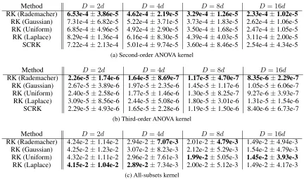
shift-Method D= 2d D= 4d D= 8d D= 16d RK (Rademacher) 6.53e-4±3.86e-5 4.62e-4±2.19e-5 3.29e-4±1.26e-5 2.33e-4±1.02e-5

RK (Gaussian) 7.31e-4±6.82e-5 5.22e-4±3.71e-5 3.73e-4±1.83e-5 2.62e-4±1.06e-5 RK (Uniform) 6.85e-4±4.96e-5 4.92e-4±2.90e-5 3.50e-4±1.68e-5 2.47e-4±1.05e-5 RK (Laplace) 8.29e-4±1.36e-4 6.16e-4±8.30e-5 4.39e-4±4.03e-5 3.11e-4±2.00e-5 SCRK 7.22e-4±2.13e-4 5.01e-4±9.74e-5 3.60e-4±8.46e-5 2.54e-4±4.34e-5

(a) Second-order ANOVA kernel

Method D= 2d D= 4d D= 8d D= 16d

RK (Rademacher) 2.26e-5±1.74e-6 1.64e-5±8.69e-7 1.17e-5±4.70e-7 8.35e-6±2.29e-7 RK (Gaussian) 2.67e-5±3.89e-6 1.97e-5±2.35e-6 1.45e-5±1.17e-6 1.05e-5±6.06e-7 RK (Uniform) 2.40e-5±2.58e-6 1.77e-5±1.46e-6 1.30e-5±8.25e-7 9.27e-6±3.93e-7 RK (Laplace) 3.09e-5±8.56e-6 2.44e-5±5.08e-6 1.80e-5±3.01e-6 1.31e-5±1.54e-6 SCRK 2.29e-5±4.93e-6 1.65e-5±2.28e-6 1.19e-5±1.50e-6 8.40e-6±6.73e-7

(b) Third-order ANOVA kernel

Method D= 2d D= 4d D= 8d D= 16d

RK (Rademacher) 4.24e-2±1.14e-2 2.94e-2±7.07e-3 2.01e-2±4.79e-3 1.49e-2±4.94e-3 RK (Gaussian) 4.25e-2±1.23e-2 3.07e-2±8.23e-3 2.12e-2±5.29e-3 1.54e-2±4.79e-3 RK (Uniform) 4.32e-2±1.11e-2 2.96e-2±7.61e-3 1.99e-2±5.05e-3 1.45e-2±3.93e-3 RK (Laplace) 4.15e-2±1.04e-2 2.89e-2±7.34e-3 2.00e-2±5.12e-3 1.49e-2±4.17e-3

(c) All-subsets kernel

Table 1: Absolute errors of RK feature maps for second-order ANOVA kernel, third-order ANOVA kernel, and all-subsets kernel using different distributions for Movielens 100K dataset.

invariant kernel, when ordermis even,σ is unfortunately meaningless in the proposed RK feature map for them-order ANOVA kernel case because Km

A(−ω,x) = KAm(ω,x). Therefore, the SCRK feature map for an even-order ANOVA kernel may not be effective.

5 Relationship between FMs and RK Feature

Map for the ANOVA Kernel

The equation for linear models using the RK feature map for the second-order ANOVA kernelZRK(x)is:

fLM(ZRK(x); ˜w) = √1

D

D X

s=1

˜

wsKA2(ωs,x), (14)

wherew˜ ∈RDis the weight vector for the RK feature map

ZRK(x). Hence, linear models using the RK feature map can be regarded as FMs with λ = ˜w/√D and only one learnable parameterλ and without the linear term. There-fore, theoretical results that guarantee the generalization er-ror of linear models using the RK map can be applied to the theoretical analysis of that of FMs. We leave this to future work. The same relationship holds between linear models using the RK feature map for the all-subsets kernel and the all-subsets model. Interestingly, it also holds between linear models using the RM feature map for the polynomial kernel and multi-convex PNs, which are multi-convex formulation models of PNs (Blondel et al. 2016b).

6 Evaluation

We first evaluated the accuracy of our proposed RK feature map on the Movielens 100K dataset (Harper and Konstan

2016), which is a dataset for recommender systems. The age, living area, gender, and occupation of users and the genre and release year of items were used as features in the same way as Blondel et al. (Blondel et al. 2016a). The dimension of the feature vectors was78.

We calculated the absolute error of the approximation of ANOVA kernels (m= 2or3) and all-subsets kernel on the training datasets. Each feature vector was normalized by its L1 _{norm. Only}₁₀_,₀₀₀_{instances were used. We calculated} the mean absolute errors for these instances for 100 trials using Rademacher, Gaussian, Uniform, and Laplace distri-butions in the RK feature maps and compared the results. For the ANOVA kernels, we also compared them with the SCRK feature map. We varied the dimension of the ran-dom features: 2,4,8 and16 times that of the original fea-ture vectors. We used Scipy (Jones, Oliphant, and Peterson 2001) implementations of FFT and IFFT (scipy.fftpack) in the SCRK and TS feature maps.

(6)

103

Number of original features (d) 2

4 6 8 10

Time (s)

RK SCRK

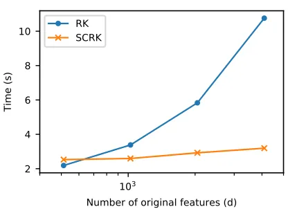
Figure 1: Comparison of mapping times of RK and SCRK feature maps for second-order ANOVA kernel with different dimensions of original feature vector for synthesis dataset (d is shown in log scale).

We next evaluated the effectiveness of the SCRK fea-ture map, which is more time and memory efficient than the RK one w.r.t the dimension of the original feature vec-tor. We created synthesis data with various dimensions of the original features and compared the mapping times of the SCRK and RK feature maps for the second-order ANOVA kernel. We usedN(0,1)as the distribution of original fea-tures and changed the dimension of the original feafea-tures: d = 512, 1024, 2048 and4096. We set D = 8092for alld.

As shown in Figure 1, when the dimension of the origi-nal feature vectordwas large, the SCRK feature map was more efficient. Although the running time of the RK fea-ture map increased linearly w.r.td, that of the SCRK feature map increased logarithmically. However, whend= 512, the RK feature map was faster than the SCRK feature map. This may be because of the following reasons. First, the differ-ence betweendandlogdis small, ifdis small. Furthermore, the SCRK feature map requires FFT and IFFT, and hence its dropped constants in Big-O notation are larger than that of the RK feature map.

We next evaluated the performance of linear models us-ing our proposed RK/SCRK feature maps for the Movie-lens 100K dataset. We converted the recommender system problem to a binary classification problem. We binarized the original ratings (from1to5) by using5as a threshold. There were 21,200,1,000, and 20,202 training, validation, and testing examples. We normalized each feature vector and varied the random features dimension in a manner similar to that used in the first evaluation. We compared the accura-cies and learning and testing times for linear SVMs using the proposed RK feature map for the ANOVA/all-subsets ker-nel, for linear SVMs using the SCRK feature map for the ANOVA kernel, for non-linear SVMs with the ANOVA/all-subsets kernel, and form-order FMs, and for the all-subsets model. Although there was a linear term in the original FMs,

we ignored it because using it or not had little effect on ac-curacy. All the methods have a regularization hyperparam-eter, which we set on the basis of the validation accuracy of the non-linear SVMs. For the linear SVMs using dom feature maps, we ran ten trials with a different ran-dom seed for each trial and calculated the mean of the val-ues. We used a Rademacher distribution for the random vec-tors. For the FMs and all-subsets model, we also ran ten trials and calculated the mean of the values. We used co-ordinate descent (Blondel et al. 2016a) as the optimization method. Because this optimization requires many iterations and much time, we ran the optimization process for the same length of time used for the non-linear SVMs. For the rank hyperparameter, we followed Blondel et al. (Blondel et al. 2016a) and set it to30. We usedLinearSVC andSVCin scikit-learn (Pedregosa et al. 2011) as implementations of linear SVMs and non-linear SVMs.LinearSVCused liblin-ear (Fan et al. 2008) andSVCused libsvm (Chang and Lin 2011). For the implementation of FMs, we used Factoriza-tionMachineClassifierin polylearn (Niculae 2016).

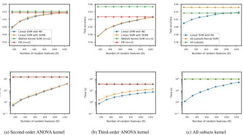
As shown in the Figure 2, when the number of random features D = 1,248 = 16d, the accuracies of the linear SVMs using the proposed RK feature map were as good as those of the non-linear SVMs, FMs, and all-subsets model. Furthermore, even though D = 1,248, their training and testing times were 2–5 times less than those of the non-linear SVMs, FMs, and all-subsets model. Because the dimension of the original feature vector was small, the running times of the linear SVMs using the SCRK feature map were longer than those of the linear SVMs using the RK feature map whenm = 3. The accuracies of the linear SVMs using the SCRK feature map were as good as those of the linear SVMs using the RK feature map, and the SCRK feature map re-quired onlyO(Dlogd)time.

We also compared the accuracies and learning and test-ing times among random-feature-based methods for the polynomial-like kernel: linear SVMs using the proposed RK/SCRK feature map for the ANOVA kernel, TS feature map, and the RM feature map for the polynomial kernel. Similar to the evaluation above, we set the regularization pa-rameter on the basis of the validation accuracy of the non-linear SVMs (we also ran the polynomial kernel SVMs). We again ran ten trials with a different random seed for each trial and calculated the mean of the values.

(7)

200 400 600 800 1000 1200 Number of random features (D) 0.56

0.58 0.60 0.62 0.64 0.66

Test accuracy Linear SVM with RK

Linear SVM with SCRK ANOVA Kernel SVM (m=2) FM (m=2)

0.58 0.60 0.62 0.64 0.66

Test accuracy Linear SVM with RK

Linear SVM with SCRK ANOVA Kernel SVM (m=3) FM (m=3)

0.58 0.60 0.62 0.64 0.66

Test accuracy

Linear SVM with RK All-subsets Kernel SVM All-subsets

200 400 600 800 1000 1200 Number of random features (D) 10−1

100 101 102

Time (s)

(a) Second-order ANOVA kernel

100 101 102

Time (s)

(b) Third-order ANOVA kernel

100 101 102

Time (s)

(c) All-subsets kernel

Figure 2: Test accuracies and times for linear SVM using RK feature map approximating (a) second-order ANOVA kernel, (b) third-order ANOVA kernel, and (c) all-subsets kernel and for two existing methods for Movielens 100K dataset. Upper graphs show test accuracies; lower ones show training and test times (time is shown in log scale).

200 400 600 800 1000 1200

Number of random features (D)

0.57 0.58 0.59 0.60 0.61 0.62 0.63 0.64

Test accuracy Linear SVM with RK Linear SVM with SCRK Linear SVM with TS Linear SVM with RM

200 400 600 800 1000 1200

Number of random features (D)

10−1

100

101

102

Time (s)

Figure 3: Test accuracies and times for linear SVM using RK/SCRK feature map approximating second-order ANOVA kernel and linear SVM using RM/TS feature map approximating second-order polynomial kernel for Movielens 100K dataset. Left graph shows test accuracies; right one shows training and test times (time is shown in log scale).

We also evaluated the performance of the linear models using the RK/SCRK feature maps and the existing models for the phishing and IJCNN datasets (Mohammad, Thabtah, and McCluskey 2012; Prokhorov 2001). The experimental results were similar to those for the Movielens 100K dataset.

7 Conclusion

(8)

Rademacher distribution but also with other distributions with zero mean and unit variance. Furthermore, we showed that the Rademacher distribution achieves the min-max op-timal variance both theoretically and empirically. We also showed how to efficiently compute the random kernel fea-ture map for the ANOVA kernel by using a signed circulant matrix projection technique. Our evaluation showed that lin-ear models using the proposed random kernel feature map are good alternatives to factorization machines and kernel methods for several classification tasks.

Acknowledgement

This work was supported by Global Station for Big Data and Cybersecurity, a project of Global Institution for Collabora-tive Research and Education at Hokkaido University. Ky-ohei Atarashi acknowledges support from JSPS KAKENHI Grant Number JP15H05711. Subhransu Maji acknowledges support from NSF via the CAREER grant (IIS 1749833).

References

Blondel, M.; Fujino, A.; Ueda, N.; and Ishihata, M. 2016a. Higher-order factorization machines. InAdvances in Neural Information Processing Systems (NIPS), 3351–3359. Blondel, M.; Ishihata, M.; Fujino, A.; and Ueda, N. 2016b. Polynomial networks and factorization machines: New in-sights and efficient training algorithms. In International Conference on Machine Learning (ICML).

Chang, C.-C., and Lin, C.-J. 2011. Libsvm: a library for support vector machines. ACM Transactions on Intelligent Systems and Technology2(3):27.

Cucker, F., and Smale, S. 2002. On the mathematical foun-dations of learning. Bulletin of the American mathematical society39(1):1–49.

Fan, R.-E.; Chang, K.-W.; Hsieh, C.-J.; Wang, X.-R.; and Lin, C.-J. 2008. Liblinear: A library for large linear clas-sification. Journal of Machine Learning Research9:1871– 1874.

Feng, C.; Hu, Q.; and Liao, S. 2015. Random feature map-ping with signed circulant matrix projection. In Interna-tional Joint Conference on Artificial Intelligence (IJCAI), 3490–3496.

Fukui, A.; Park, D. H.; Yang, D.; Rohrbach, A.; Darrell, T.; and Rohrbach, M. 2016. Multimodal compact bilin-ear pooling for visual question answering and visual ground-ing. InEmpirical Methods in Natural Language Processing (EMNLP).

Harper, F. M., and Konstan, J. A. 2016. The movielens datasets: history and context.ACM Transactions on Interac-tive Intelligent Systems5(4):19.

Jones, E.; Oliphant, T.; and Peterson, P. 2001. Scipy: Open source scientific tools for python.

Kar, P., and Karnick, H. 2012. Random feature maps for dot product kernels. InArtificial Intelligence and Statistics (AISTAS), 583–591.

Le, Q.; Sarl´os, T.; and Smola, A. 2013. Fastfood-approximating kernel expansions in loglinear time. In In-ternational Conference on Machine Learning (ICML). Lin, T.-Y.; RoyChowdhury, A.; and Maji, S. 2015. Bilinear cnn models for fine-grained visual recognition. In Interna-tional Conference on Computer Vision (ICCV).

Livni, R.; Shalev-Shwartz, S.; and Shamir, O. 2014. On the computational efficiency of training neural networks. In Advances in Neural Information Processing Systems (NIPS), 855–863.

Mohammad, R. M.; Thabtah, F.; and McCluskey, L. 2012. An assessment of features related to phishing websites us-ing an automated technique. In International Conference for Internet Technology And Secured Transactions (ICITST), 492–497.

Niculae, V. 2016. A library for factorization machines and polynomial networks for classification and regression in python. https://github.com/scikit-learn-contrib/polylearn/. Novikov, A.; Trofimov, M.; and Oseledets, I. 2016. Ex-ponential machines. International Conference on Learning Representations Workshop.

Pagh, R. 2013. Compressed matrix multiplication. ACM Transactions on Computation Theory5(3):9.

Pedregosa, F.; Varoquaux, G.; Gramfort, A.; Michel, V.; Thirion, B.; Grisel, O.; Blondel, M.; Prettenhofer, P.; Weiss, R.; Dubourg, V.; et al. 2011. Scikit-learn: Machine learning in python.Journal of Machine Learning Research12:2825– 2830.

Pham, N., and Pagh, R. 2013. Fast and scalable polyno-mial kernels via explicit feature maps. InInternational Con-ference on Knowledge Discovery and Data Mining (KDD), 239–247.

Prokhorov, D. 2001. IJCNN 2001 neural network competi-tion. Slide Presentation in IJCNN.

Rahimi, A., and Recht, B. 2008. Random features for large-scale kernel machines. InAdvances in Neural Information Processing Systems (NIPS), 1177–1184.

Rendle, S. 2010. Factorization machines. InInternational Conference on Data Mining (ICDM), 995–1000.