ISSN: 1137-3601 (print), 1988-3064 (on-line) ©IBERAMIA and the authors
INTELIGENCIA ARTIFICIAL
http://journal.iberamia.org/
On the Enhancement of Classification Algorithms Using Biased
Samples
Safaa O. Al-mamory
College of Business Informatics, University of Information Technology and Communications, Baghdad, Iraq [email protected]
Abstract Classification algorithms' performance could be enhanced by selecting many representative points to be included in the training sample. In this paper, a new border and rare biased sampling (BRBS) scheme is proposed by assigning each point in the dataset an importance factor. The importance factor of border points and rare points (i.e. points belong to rare classes) is higher than other points. Then the points are selected to be in the training sample depending on these factors. Including these points in the training sample enhances classifiers experience. The results of experiments on 10 UCI machine learning repository datasets prove that the BRBS algorithm outperforms many sampling algorithms and enhanced the performance of several classification algorithms by about 8%. BRBS is proposed to be easy to configure, covering all points space, and generate a unique samples every time it is executed.
Keywords: Classification, LOF, Decision Boundary, Biased Sampling, imbalanced dataset.
1
Introduction
The diverse applications of classification algorithms encouraged researchers to enhance the performance of these algorithms; these applications include customer target marketing [1], medical disease diagnosis [2], supervised event detection [3], multimedia data analysis [4], biological data analysis [5], document categorization and filtering [6], and social network analysis [7]. However, enhancing classifiers performance is a challenging mission. There are several ways to improve classifier's accuracy such as preprocess dataset [8], enhancing algorithms performance, and post-process the classifiers’ results [9]. Data sampling is one of data preprocessing techniques. This paper boosts the classification algorithms by enhancing selection of training sample as a preprocess step.
Uniform distributions and dataset with one level of density are rare in real applications. Some records may be of more value in the sample than others; knowing points' importance could help in sampling by assigning an importance value for each point. Having points' importance helps in obtaining representative samples which in turn enhances classifier's performance. Most of the existing sampling algorithms neglect representing small clusters in the sample. In this paper, Border and Rare Biased Sampling Algorithm (BRBS) is proposed in which the border points and rare class points are more important than others. We will use point and instance terms interchangeably.
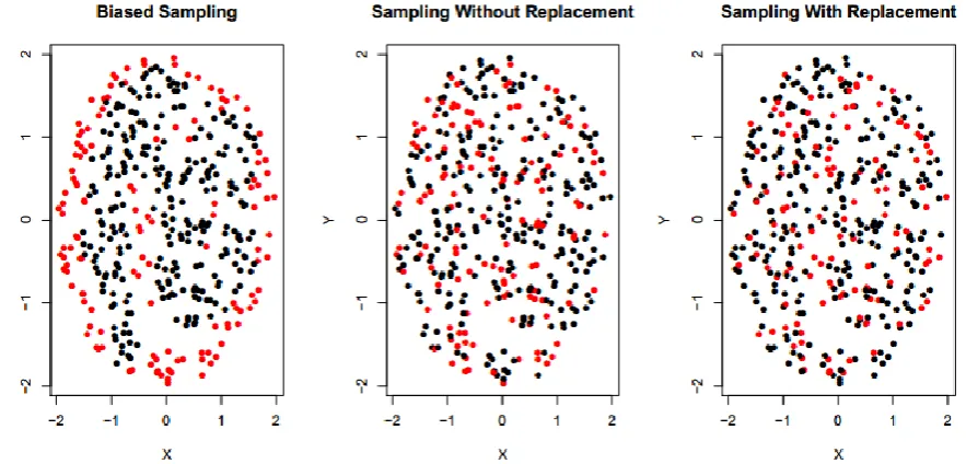
sampling without replacement algorithms are not biased as can be seen in the figure. The main contribution of this paper is to suggest a sampling mechanism, depending on LOF, to ensure rare classes and border points' coverage. The experiments on 10 different datasets with three classifiers prove that BRBS has outperformed holdout sampling and cross validation and enhanced different classifiers performance by about 8% (on average).
Figure. 1: visual comparison between BRBS, sampling without replacement, and sampling with replacement on synthesized dataset
This paper is organized as follows. The related work is presented Section 2. Section 3 states the proposed algorithm. The experimental results are presented in Section 4. Finally, Section 5 concludes this paper.
2
Related Work
In the last few decades, the research community has studied precisely the sampling in order to improve classification and clustering performance. The first group of researchers worked on biased sampling to force the sample to have points from dense regions of data more than the points from sparse regions. In other words, they generate samples that allow clustering processes to find clusters more accurately. George Kollios et al. [10] proposed a density-biased sampling by calculating the density of the local space around each point and then place the point in the sample with probability that is a function of local density. They chose kernel function for density estimation and applied their method to cluster and outlier detection problems. Ana Paula Appel et al. [11] presented a biased box sampling algorithm using local density. The technique is based on a multi-dimensional and multi-resolution grid structure where its depth depends on points' local density of the related region. Christopher R. Palmer [12] used a weighted sample in order to preserve the data density. They introduce a sampling technique to improve on uniform sampling when skewed clusters are processed. A hashing function is used when doing a biased sampling to map bins in space to a linear ordering. An incremental algorithm is introduced by Frédéric Ros et al. [13] to combine distance and density concepts. They manage distance concepts in order to make sure space coverage and fit cluster shapes by selecting representative points in every cluster.
borderline points of the minority class are easier to be misclassified than those points away from the borderline. Thus, they oversampled points of the minority class at the borderline.
The third group of researchers focused on random sampling to enhance classifiers' performance. The holdout algorithm samples the data randomly into two samples which are 66% for training and 34% for testing (these percent are approximated) [19]. Random subsampling approach apply hold-out method several times to boost the estimation of a classifier performance [19]. Cross-validation (CV) is an alternative to random subsampling, in which each record is used the same number of time for training and once only for testing [19]. The idea of the bootstrap is to sample the dataset with replacement to form a training set [20].
The proposed method is different from all previous work in two folds. The first fold is that it is uses local outlier factor as a guide for the sampling. Unlike the previous work in which the work was biased to select from denser regions more than sparse regions, the second fold is that it is biased towards selecting border points and rare class points to be in the sample. To the best of our knowledge, this is the first paper uses importance scoring of points in the sampling.
3
The Proposed Algorithm
The performance of any classifier could be improved if the training examples are representative. The sample containing instances from rare classes and border points is more representative than simple random sampling. Subsection 3.1 describes the concept of local outlier factor while Sunsection 3.2 states how to use that concept of local outlier factor in enhancing sampling.
3.1
Local Outlier Factor
An outlier is an observation that deviates so much from other observations as to arouse suspicion that it was generated by a different mechanism [21]. Three different techniques to detect outliers are available which are supervised, semi-supervised, and unsupervised [22]. LOF [23] is a density based and unsupervised algorithm which gives a numeric value for each point representing the outlier factor. The normal value is 1; the higher the value is the outlier the point is. In this paper, LOF algorithm is used as a base algorithm to rank points. LOF has one control parameter, MinPts. The remaining of this subsection will present the main concepts of LOF algorithm.
To detect density-based outliers, it is necessary to compare the densities of different sets of objects, which means that we have to determine the density of sets of objects dynamically. Therefore, we keep MinPts as the only parameter and use the values reach-distMinPts(p, o), for o ∈ N MinPts(p), as a measure of the volume to determine the density in the neighborhood of an object p. Intuitively, the local reachability density of an object p is the inverse of the average reachability distance based on the MinPts nearest neighbors of p. Equ. 1 presents the local reachability distance [23].
(1)
The outlier factor of object p captures the degree to which we call p an outlier. It is the average of the ratio of the local reachability density of p and those of p’s MinPts-nearest neighbors. It is easy to see that the lower p's local reachability density is, and the higher the local reachability densities of p's MinPts-nearest neighbors are, the higher is the LOF value of p. The (local) outlier factor of p is defined as in Equ. 2 [23].
(2)
where lrd() is the local reachability density of a given point with respect to MinPts, and is the list of nearest MinPts to the point p given in Equ. Z. In this paper, we will use LOF(p) or (LOF) instead
In LOF algorithm, the local density of any point is compared to the neighbors' local densities. A point is considered an outlier if its density is lower than its neighbors density. The score of LOF is approximately 1 means that the density around the point is similar to its neighbors while LOF value much larger than 1 is indicator of an outlier.
3.2
The Biased Sampling Algorithm
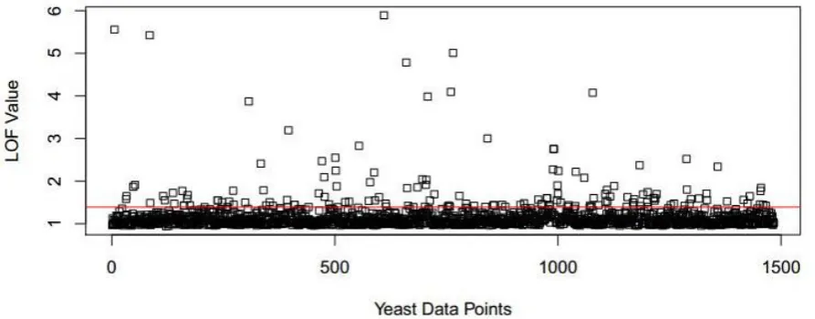
The border between two neighboring regions is known as the decision boundary [19]. The borderline points and rare points are simply misclassified compared with those ones far from the borderline. Therefore, BRBS is suggested to ensure that the training sample contain these classifiers' challenging points. To achieve this goal, an importance score is given to each point in dataset. LOF is used, in this paper, to give this score for all points. The borderline points and rare points always have high LOF score since they have less set of neighbors' points. Figure 2 depicts the LOF values for instances of Yeast dataset where the red line represents the highest 10% LOF values. Most of these 10% points are from rare and border points from different classes.
Figure 2: LOF values for Yeast instances; the red line representing 10% of the dataset
Having the highest 10% of points (having highest LOF scores) in the training sample will improve classifier performance. In this paper, the training sample will have 66% of points and the testing sample will have 34% of points. Algorithm 1 contains the pseudo code of BRBS algorithm. In general, the BRBS algorithm makes a ranking of the points according to the importance score which is computed by LOF algorithm (Lines 2 and 3). Hereafter, a holdout technique with scoring points modification is used to partition the dataset into two parts (Lines 4 and 5). Line 4 may classify noise points as border points. Therefore, it is recommended to employing one of noise removing algorithms before BRBS is applied.
Algorithm 1: pseudo code of BRBS algorithm
Algorithm BRBS (D , MinPts) Input: D , MinPts
Output: Train, Test 1. Begin
2. For each d D do
3. L(d) = Compute using Equ. 2 ; 4. Train = select 66% of points having highest L(D) score; 5. Test = select 34% of points having minimum L(D) score; 6. Return Train, Test;
BRBS uses LOF idea but apply LOF in an innovative way and have several advantages over existing sampling algorithm. It could be look for BRBS from different points of views like:
Ease of use: several sampling algorithms have many parameters to set which are more meaningful to the
data miner than to the user and hence not easy to set. BRBS classifies a point as a border point (or a rare point) depending on one control variables (i.e. MinPts). The higher MinPts value is the more border points. The best value for the parameter is selected using K-dist plot [24] curve which sorts the points according to distances. After drawing the curve, the knee in the curve reflects the best value to be selected making the algorithm easy to use.
Not random sample. The proposed sampling algorithm generates same sample every time it is executed
since it selects top n% instances as a training sample having highest LOF score. This feature is not available in random sampling (with or without replacement). In addition, it is considered as unsupervised sampling algorithm; however it is biased towards selecting rare class instances.
Space coverage. In BRBS, choosing the points with highest LOF scores ensures rare classes are represented. In addition, the points at different classes' borders are selected since their density is different from their neighbors' densities. These points represent about 10% of the dataset. Hence, it should select extra more than 50% of points to be included in the training sample.
4
Experimental Results
The main goal of this section is to do experiments to test the performance of the proposed algorithm. To achieve this goal, three sets of experiments were conducted. The first set focuses on selecting instances with the algorithm. The second set of experiments was to compare the algorithm with two most common algorithms which are hold-out sampling algorithm and cross validation algorithm. The third set of experiments conducted to evaluate the root mean square error (RMSE) of the algorithm. All experiments are conducted by R language [25] and Weka [26].
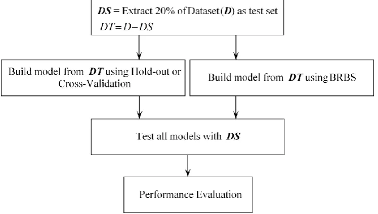
The experiment design that is used to test the performance of BRBS is shown in Figure 3 to obtain a valid comparison. A representative test set (DS) including both easy and hard points is kept apart to make the test fair. The size of DS is 20% of the given dataset. Then, the rest of the points (DT) are used as training set to learn two sets of classifiers, the first in the standard way to be used as a baseline and the second set of classifiers are learnt with the BRBS. Then, the two sets of classifiers are evaluated against the test set (DS). This setup is used with hold-out, cross-validation, and BRBS. Three different classification algorithms were selected (as base classifiers) to compare with, which are J48, Naïve Bayes, and Multi-layer perceptron. The reason for selecting these algorithms is that they used different strategies for dealing with decision boundary regions.
In order to compare BRBS and different algorithms, several measures had been used which are accuracy, recall, precision, the F measure. The accuracy is computed using (TP+TN)/(TP+TN+FP+FN) [19] where TP and TN are correctly classified points (positive and negative points, respectively) while FP and FN are incorrectly classified points (positive and negative points, respectively). Recall (TP)/(TP +FN) measures the proportion of actual positives that are correctly classified. Precision is the ratio of recognized positives which are correctly classified; it is computed by(TP)/(TP+FP). The F-measure is a mixture of recall and precision and is calculated as 2 * (Precision * Recall/( Precision + Recall)) [27]. In the presence of imbalanced datasets, it is more appropriate to use F-measure.
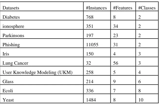
Ten different datasets have been used from UCI repository [28] as can be seen in Table 1. These datasets have different number of features and ranging from binary to multi class classification problems. In addition, these datasets are from different fields. Some of the selected datasets have rare classes like Ecoli, Yeast, and Glass; we consider classes occurred less than 10% as rare.
Table 1: The used dataset in the experiments from UCI repository
Datasets #Instances #Features #Classes
Diabetes 768 8 2
ionosphere 351 34 2
Parkinsons 197 23 2
Phishing 11055 31 2
Iris 150 4 3
Lung Cancer 32 56 3
User Knowledge Modeling (UKM) 258 5 4
Glass 214 9 6
Ecoli 336 7 8
Yeast 1484 8 10
The proposed sampling algorithm produces representative training samples for the classifiers. Each class, containing set of instances, has a set of border instances which are selected by the proposed algorithm. Furthermore, the selected samples are the more difficult instances to classify. According to 10 experiments (on datasets appeared in Table 1) to get samples from, the proposed algorithm successfully produces good samples. The percent of each class in these datasets before and after sampling is presented in Table 2. As can be seen in the table, the algorithm fairly took instances from all classes when selecting the sample. Moreover, it selects most instances in rare classes since these instances sometimes appeared to be noise. The rare classes' instances almost have biased features values so their LOF value tends to be high. Therefore the proposed algorithm selects them as can be noted from Table 2 where the instances of classes 3 and 4 from Ecoli dataset are selected entirely; more examples are bolded. It could be concluded that the proposed algorithm behavior in selecting training instances is biased toward selecting the instances from rare classes.
Table 2: Percent of classes before and after sampling in the format before(after)
Datasets Class Number
1 2 3 4 5 6 7 8 9 10
Diabetes 34.9 (24.5)
65.1 (42.2) ionosphere 35.9
(32.5) 64.1 (34.2) Parkinsons 24.6
(20)
75.4 (46.7) Phishing 55.7
(33.3) 44.3 (33.4)
Iris 33.3
(24.7) 33.3 (22.7) 33.3 (19.3) Lung Cancer 28.1 (18.8) 40.6 (21.9) 31.3 (25)
UKM 9.3
(4.3) 32.2 (19.8) 34.1 (24.8) 24.4 (17.8)
Glass 32.7
(19.2) 7.9 (4.7) 4.2 (3.3) 35.5 (26.6) 13.6 (8.4) 6.1 (4.2)
Ecoli 42.6
(29.2) 22.9 (17) 0.6 (0.6) 0.6 (0.6) 10.4
(5.7) 6 (2.1) 1.5 (1.5)
15.5 (10.1)
Yeast 16.4
(10.2) 28.9 (20.1)
31.2
(23.5) 3 (1.5) 2.4
(0.8) 3.4 (2) 11
(7.6) 2 (0.7) 1.3 (0) 0.3 (0.3)
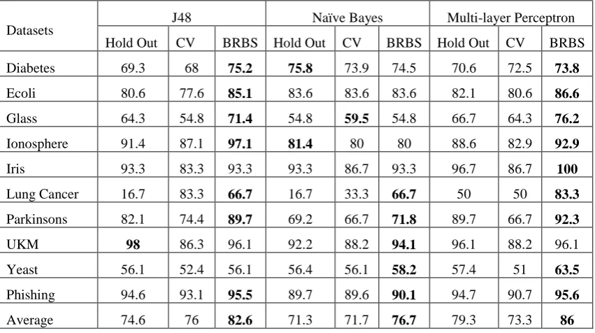
Table 3: Comparison in Accuracy measure between BRBS algorithm, hold-out, and CV algorithms with three different classification algorithms
Datasets
J48 Naïve Bayes Multi-layer Perceptron
Hold Out CV BRBS Hold Out CV BRBS Hold Out CV BRBS
Diabetes 69.3 68 75.2 75.8 73.9 74.5 70.6 72.5 73.8
Ecoli 80.6 77.6 85.1 83.6 83.6 83.6 82.1 80.6 86.6
Glass
64.3 54.8 71.4 54.8 59.5 54.8 66.7 64.3 76.2
Ionosphere 91.4 87.1 97.1 81.4 80 80 88.6 82.9 92.9
Iris 93.3 83.3 93.3 93.3 86.7 93.3 96.7 86.7 100
Lung Cancer 16.7 83.3 66.7 16.7 33.3 66.7 50 50 83.3
Parkinsons 82.1 74.4 89.7 69.2 66.7 71.8 89.7 66.7 92.3
UKM 98 86.3 96.1 92.2 88.2 94.1 96.1 88.2 96.1
Yeast 56.1 52.4 56.1 56.4 56.1 58.2 57.4 51 63.5
Phishing 94.6 93.1 95.5 89.7 89.6 90.1 94.7 90.7 95.6
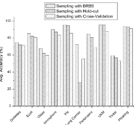
Figure 4: histogram represents a comparison of averaged accuracy measure for different sampling algorithms For computing more performance comparison measures, three measures mentioned above are calculated which are the precision, recall, and F-measures for BRBS and Hold-out. These measures for four different datasets are shown in Table 4. In this table, we can observe that BRBS has the highest precision, recall, and F-measure values while comparing with Hold-out sampling.
Table 4: Comparison between BRBS and hold-out with precision, recall, and F measure Datasets
Hold out BRBS
Precision Recall F-Measure Precision Recall F-Measure
Diabetes 0.678 0.693 0.667 0.745 0.752 0.745
Ionosphere 0.918 0.914 0.915 0.974 0.971 0.972
Iris 0.933 0.933 0.933 0.933 0.933 0.933
Yeast 0.544 0.561 0.548 0.552 0.561 0.552
Average 0.768 0.775 0.766 0.801 0.804 0.801
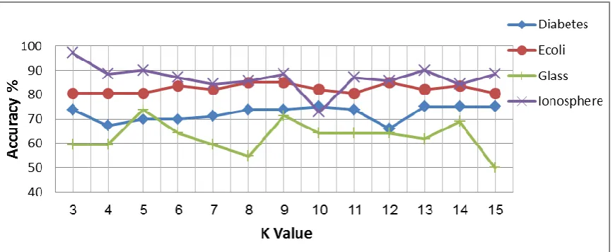
Figure 5: The influence of k parameter on accuracy value
Root mean square error (RMSE) [29] has been used here as another comparison measure to show the error rate in the BRBS algorithm and other algorithms. Equation of RMSE is stated in Equ. 3 where P is the predicted value and O is the observed one. It is well known that RMSE gives good indication as a comparison measure when the classification problem is binary. Hence, only four datasets were used in the experiment. Figure 6 depicts the results of RMSE as a comparison measure. Each column in the figure represents the average of three experiments with different sampling algorithms. The average of RMSE for all experiments was 0.33for BRBS, 0.36 for hold-out, and 0.41 for cross validation. It can be concluded from this figure that the RMSE results of BRBS algorithm is the minimum with respect to other algorithms.
(3)
whole space paying attention to rare points and borderline points as noted in Table 2. BRBS is easy to use since it has one control parameter and every point in the dataset will get constant position in the samples because the points' importance score will be the same every time the algorithm is executed.
5
Conclusions
Several limitations exist in the state of the art of sampling algorithms like multi-control parameters, biasing towards density clusters only, and others. The margin points of different classes and minority class points have a great impact on classifier’s model creation. Therefore, BRBS give these points more importance than other points in training sample building. It extracts margin points from decision boundary between classes and points from rare classes (using LOF as a scoring algorithm) to be included in the training sample to increase classifier experience. The main characteristics of BRBS are ease of use, not random samples, and space coverage.
Acknowledgements
The author recognizes and thanks the anonymous reviewer and the journal editor for their important comments and suggestions, which have significantly enhanced the paper.
References
[1] C. C. Aggarwal, Data classification : algorithms and applications. CRC Press, 2014.
[2] S. U. Ghumbre and A. A. Ghatol, “Heart Disease Diagnosis Using Machine Learning Algorithm,” in Proceedings of the International Conference on Information Systems Design and Intelligent Applications, 2012, pp. 217–225.
[3] H. Becker, “Identification and Characterization of Events in Social Media,” Columbia University, 2011. [4] N. Patel and I. Sethi, “Multimedia Data Mining: An Overview,” in Multimedia Data Mining and
Knowledge Discovery, London: Springer London, 2007, pp. 14–41.
[5] A. Tanay, S. Roded, and S. Ron, “Biclustering Algorithms for Biological Data Analysis: A Survey,” IEEE/ACM Trans. Comput. Biol. Bioinforma., vol. 1, no. 1, pp. 24–45, 2004.
[6] L. Cai and T. Hofmann, “Hierarchical document categorization with support vector machines,” in Proceedings of the thirteenth ACM international conference on Information and knowledge management, 2005, pp. 78–87.
[7] J. Kim and M. Hastak, “Social network analysis: Characteristics of online social networks after a disaster,” Int. J. Inf. Manage., vol. 38, no. 1, pp. 86–96, 2018.
[8] S. O. Al-Mamory, “Classification performance enhancement using boundary based sampling algorithm,” in Annual Conference on New Trends in Information and Communications Technology Applications, 2017, pp. 186–191.
[9] E. B. Kong and T. G. Dietterich, “Error-Correcting Output Coding Corrects Bias and Variance,” Mach. Learn. Proc., pp. 313–321, 1995.
[10] G. Kollios, D. Gunopulos, N. Koudas, and S. Berchtold, “Efficient biased sampling for approximate clustering and outlier detection in large data sets,” IEEE Trans. Knowl. Data Eng., vol. 15, no. 5, pp. 1170–1187, Sep. 2003.
[11] A. P. Appel, A. A. Paterlini, E. P. M. de Sousa, A. J. M. Traina, and C. Traina, “A Density-Biased Sampling Technique to Improve Cluster Representativeness,” pp. 366–373, 2007.
[12] C. R. Palmer and C. Faloutsos, “Density Biased Sampling: An Improved Method for Data Mining and Clustering,” ACM SIGMOD Int. Conf. Manag. Data, no. 82, pp. 82–92, 2000.
[13] F. Ros and S. Guillaume, “DENDIS: A new density-based sampling for clustering algorithm,” Expert Syst. Appl., vol. 56, pp. 349–359, 2016.
[14] N. V Chawla, K. W. Bowyer, L. O. Hall, and W. P. Kegelmeyer, “SMOTE : Synthetic Minority Over-sampling Technique,” J. Artif. Intell. Res., vol. 16, no. 1, pp. 321–357, 2002.
[16] G. Liu, Y. Yang, and B. Li, “Fuzzy rule-based oversampling technique for imbalanced and incomplete data learning,” Knowledge-Based Syst., vol. 158, pp. 154–174, 2018.
[17] G. Douzas, F. Bacao, and F. Last, “Improving imbalanced learning through a heuristic oversampling method based on k-means and SMOTE,” Inf. Sci. (Ny)., vol. 465, pp. 1–20, 2018.
[18] H. Han, W.-Y. Wang, and B.-H. Mao, “Borderline-SMOTE: A New Over-Sampling Method in Imbalanced Data Sets Learning,” LNCS, vol. 3644, pp. 878 – 887, 2005.
[19] T. P, M. Steinbach, A. Karpatne, and K. Vipin, Introduction to data mining, 2nd ed. Pearson, 2018. [20] I. H. Witten and E. Frank, Data Mining: Practical Machine Learning Tools and Techniques. Morgan
Kaufmann, 2005.
[21] D. M. Hawkins, Identification of Outliers. Dordrecht: Springer Netherlands, 1980.
[22] V. Chandola, A. Banerjee, and V. Kumar, “Anomaly Detection: A Survey,” ACM Comput. Surv., vol. 41, no. 3, pp. 1–58, 2009.
[23] M. M. . Breuniq, H.-P. . Kriegel, R. T. . Ng, and J. . Sander, “LOF: Identifying density-based local outliers,” SIGMOD Rec. (ACM Spec. Interes. Gr. Manag. Data), vol. 29, no. 2, pp. 93–104, 2000.
[24] M. Ester, H.-P. Kriegel, J. Sander, and X. Xu, “A Density-based Algorithm for Discovering Clusters a Density-based Algorithm for Discovering Clusters in Large Spatial Databases with Noise,” in Proceedings of the Second International Conference on Knowledge Discovery and Data Mining, 1996, pp. 226–231.
[25] S. Urbanek and M. Plummer, “R: The R Project for Statistical Computing.” [Online]. Available: https://www.r-project.org/. [Accessed: 15-Apr-2019].
[26] M. Hall, E. Frank, G. Holmes, B. Pfahringer, P. Reutemann, and I. H. Witten, “The WEKA Data Mining Software: An Update,” ACM SIGKDD Explor. Newsl., vol. 11, no. 1, p. 10, Nov. 2009.
[27] Y. F. Roumani, J. H. May, D. P. Strum, and L. G. Vargas, “Classifying highly imbalanced ICU data,” Health Care Manag. Sci., vol. 16, no. 2, pp. 119–128, Jun. 2013.
[28] UC Irvine, “UCI Machine Learning Repository.” [Online]. Available: https://archive.ics.uci.edu/ml/index.php. [Accessed: 02-Mar-2019].