1
ESTIMATION AND VALIDATION OF INTERFACIAL HEAT TRANSFER
COEFFICIENT DURING SOLIDIFICATION OF SPHERICAL SHAPED
ALUMINUM ALLOY (AL 6061) CASTING USING INVERSE CONTROL
VOLUME TECHNIQUE
L. Anna Gowsalya
a,
P.D. Jeyakumar
b*,
R. Rajaraman
c†and R. Velraj
daResearch Scholar, Department of Mechanical Engineering, School of Mechanical Sciences, B.S. Abdur Rahman Crescent Institute of Science and Technology, Vandalur, Chennai, Tamilnadu, India- 600 048, E-mail: [email protected]
bAssociate Professor, Department of Mechanical Engineering, School of Mechanical Sciences, B.S. Abdur Rahman Crescent Institute of Science and Technology, Vandalur, Chennai, Tamilnadu, India- 600 048, E-mail: [email protected]
cProfessor, Department of Mechanical Engineering, School of Mechanical Sciences, SRM Institute of Science and Technology, Vadapalani Campus, Chennai, Tamilnadu, India- 600 026. Email: [email protected]
dProfessor and Director, Institute for Energy Studies, College of Engineering Guindy, Anna University, Chennai, Tamilnadu, India- 600 025, Email: [email protected]
A
BSTRACTSolidification of casting is a complex phenomenon which requires accurate input to simulate for real time applications. Interfacial heat transfer coefficient (IHTC) is an important input parameter for the simulation process. The IHTC is varying with respect to time during solidification and the exact value is to be given as input for the accurate simulation of the casting process. In this work an attempt is made to estimate the IHTC during solidification of spherical shaped aluminum alloy component with sand mould. The mould surface heat flux and mould surface temperatures are estimated by inverse control volume technique using the temperature measured at different locations in the mould. The IHTC is calculated using these values. The estimated value of mould surface temperature is validated with the available measured mould temperature at specified location using direct heat conduction problem.
Keywords: Solidification, Aluminum alloy, IHTC, IHCP, control volume.
1.
I
NTRODUCTIONDuring the solidification of casting process, there is an air gap formation between the metal and the mould due to shrinkage of solidifying metal. This air gap acts as a barrier for the heat to flow from the cast metal to the mould. The heat transfer between the cast and the mould is one of the important parameter that influences the solidification time, cooling rate and quality of the casting. This heat transfer rate has been dependent on various factors like thickness of surface coatings, casting size, chill or mould material, applied pressure, alloy type and composition, liquid alloy surface tension, mould and chill preheat, alloy superheat and chill surface roughness etc. These factors make the solidification phenomenon more complex and difficult to analyze the heat transfer at the metal-mould interface. The drop in temperature between the cast surface and the mould surface is represented by an important parameter called interfacial heat transfer coefficient (IHTC). Predicting the heat transfer at the metal – mould interface is one of the important boundary conditions during the solidification.
Most of the commercial software’s available for the solidification process should provide reliable results only when the correct material properties and the initial and boundary values are given. The current commercially available software assumes constant value of IHTC (film
*Corresponding author: Email: [email protected] †Corresponding author: Email: [email protected]
coefficient). However the IHTC is not constant during the solidification process and it varies with time. Hence there is a need for estimation of accurate value of interfacial heat transfer coefficient for different geometries. This paper deals with the estimation IHTC using inverse control volume technique for spherical shaped Aluminum alloy cast part with surrounding sand mould.
During the solidification of casting process the surface heat flux and the mould surface temperature are varying with respect to time. These two are the primary factors acting as boundary conditions for the evaluation of interfacial heat transfer coefficient. The surface heat flux and the mould surface temperature are calculated with the help of the thermocouple conveniently placed some distance away from the mould surface. Since the boundary condition described here is the “cause” (surface heat flux) is calculated from the “effect” measured temperature histories at different locations on the mould surface during solidification of casting (Grysa, 2011; Ozisik et al., 2004). Therefore from the effect (measured temperature histories), the cause at the metal mould interface (surface heat flux or temperature) is calculated which makes the problem as an inverse heat conduction problem (IHCP). The IHCP is also known as Ill posed problem. The direct heat conduction problems or well posed problem is one in which the effect is calculated from the known boundary condition. Generally the analysis of solidification of casting process falls under inverse heat conduction problem (Ozisik et al., 2004).
Frontiers in Heat and Mass Transfer
Many authors tried the varieties of numerical solution for the IHCP due to the fast development in computer applications. There are 14 solution methodologies are available to solve the IHCP but the selection of a particular method is mainly based on easy programming. Some of the numerical methods for IHCP are Finite Difference Method (FDM), Finite Element Method (FEM), Finite Volume Method (FVM) and Control Volume Technique. The other methods available are genetic algorithm, Becks function specification method and lumped capacitance method etc. (Grysa, 2011).
The solution for an inverse heat conduction problem (IHCP) of the solidification of casting at the metal –mould interface is based on the minimization of the objective function containing both estimated and measured temperatures (Beck et al., 1977). Sahin (Sahin et al., 2006) has reported, the estimation of IHTC for cylindrical geometry aluminum alloy casting with two different mould materials copper and HS13 steel using FDM. The upward directional solidification is mainly affected by the contact area and roughness of the material. The IHTC value was very high when pouring the material in liquid stage and during solidification it dropped down. The value of IHTC ranged from 19 - 9.5 kW/m2 K for
copper and for HS13, it ranged from 6.5 – 5 kW/m2 K.
The IHTC is very much affected by the release of latent heat and evaporation of moisture content of green sand during solidification. These characteristics are analyzed by Chao (Chao et al., 2007) for the Aluminum and Tin- lead alloys using lump capacitance method and they reported that the peak value of IHTC was due to the latent heat release of molten material.
The increase in initial temperature of a coated material increases the IHTC and increasing the die coating thickness resulted in reduction of IHTC by Hallam (Hallam, 2004). A decreasing trend of IHTC was observed when the temperature of the contacting metal with the mould decreased was reported by Bezhenov (Bezhenov et al., 2017). Jose (Jose et al., 2006) evaluated transient heat transfer coefficient using control volume technique for Al-Si alloys by comparing the experimental data with the theoretical temperature profile of a numerical model.
Ranjbar (Ranjbar et al., 2009) estimated the IHTC by optimizing the solidification experiment and using inverse heat conduction problem. They performed experiment on Sn-10%Pb alloy in a metallic mould and used a Conjugate Gradient Method (CGM). Zhang et al., 2013, estimated the interfacial heat flux for cylindrical shaped casting and verified the accuracy of the solution by comparing the temperature data obtained from commercial ProCast software. Zhang (Zhang et al., 2013) developed a model to determine IHTC between casting and metal chill by measuring temperatures in the chill, cast and using the inverse heat conduction method. They also verified the experimental temperatures with the numerically calculated temperatures using FEA and found good agreements.
Zhang (Zhang et al., 2017) conducted a detailed study for a heat transfer phenomena on the solidification of 5 step squeeze casting of wrought aluminum alloy with a different hydraulic pressure. The authors observed that the increase in hydraulic pressure increases the IHTC values due to the reduction in the gap between the solidifying metal and die surface. Vaisleiou (Vaisleiou et al., 2017) developed a genetic algorithm (GA) approach to determine the value of heat transfer coefficient (HTC) between Al-Si cast and steel mould, considering two different geometries. The GA simulated the temperature by getting the different values of HTC as input and the simulation continued until there was a small difference between simulated and actual measured temperature being obtained.
Few research papers are available for comparing the results of two different inverse approaches. Rajaraman (Rajaraman and Velraj, 2008) estimated and compared the IHTC results for cylindrical geometry casting with sand mould using Beck’s function specification approach and control volume approach. They reported that the control volume approach gives accurate results as it does not involve iterative processes. Rajaraman (Rajaraman et al., 2018) also estimated IHTC for rectangular geometry aluminum alloy casting using two different inverse methods.
The results obtained by both the inverse methods have identical trend in many places with minimum deviation in some regions.
From the literature it is found that many researchers considered various geometries, materials and solution techniques for the estimation of IHTC. The value of IHTC is also differs based on the geometry, thickness, materials and types of coatings etc. Only very few researchers validated the IHTC obtained. In this paper an attempt is made to estimate the IHTC between the spherical shaped Aluminum alloy casting and spherical shaped sand mould during the solidification. The estimated mould surface temperature is given as input for the direct heat conduction problem to validate the results of IHCP.
2.
P
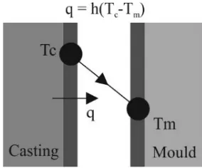
ROBLEM DEFINITIONThe IHTC has a major influence on the heat transfer between the metal and the mould. The schematic representation of IHTC during solidification of casting is shown in Fig. 1.
Fig. 1 Schematic representation of IHTC during solidification of casting
The heat transfer at the metal mould interface is calculated based on mould surface and cast surface temperatures as given by equation (1):
𝑞𝑞(𝑡𝑡) =ℎ(𝑡𝑡)[𝑇𝑇𝑐𝑐(𝑡𝑡)− 𝑇𝑇𝑚𝑚(𝑡𝑡)] (1)
Where q (t) is heat flux at the mould surface (W/m2), h(t) is
interfacial heat transfer coefficient (W/m2°C) , Tc(t) cast surface
temperature (°C) and Tm(t) mould surface temperature (°C)
3.
SOLIDIFICATION OF RECTANGULAR
GEOMETRY CASTING
Fig. 2 Experimental set up for acquiring temperature data from cast and mould
3 spherical cavity of 30 mm diameter was prepared in the green sand using split pattern, the runner and risers were located at appropriate locations. The entire outer surface of the mould was exposed to atmosphere to ensure one dimensional heat transfer. There were four K type thermocouples used to acquire the temperature history from the cast and the mould. One thermocouple was directly inserted at convenient location and nearby the cast surface to measure the cast temperature. This temperature was taken as cast surface temperature of the solidifying metal due to high thermal conductivity of Aluminum alloy. The remaining three thermocouples were located in the mould at distances of 20, 30 and 40 mm from the mould surface to measure the temperature of the mould with respect to time. All these thermocouples were connected to a 16 channel NI 9213 data acquisition system interfaced with a computer and LABVIEW software to measure the temperatures on the cast and the mould as shown in Fig.2.
4.
M
ELTING ANDP
OURINGThe Al 6061 aluminum alloy is melted in a 15 kW, 10 kg electric furnace with high degree of super heat. The high degree of superheat was maintained to avoid solidification of cast metal during pouring and to maintain good fluidity. The melted alloy was poured into the spherical cavity mould, the temperatures were recorded by data acquisition system (DAQ) for every 3 sec and stored in computer till solidification process was complete. This data acquired process continued till the temperature difference between the mould and atmosphere was significantly less. The properties of cast metal and sand mould are listed in table1.
Table 1. Properties of Aluminum alloy and Green sand.
Material Density kg/m3 Specific heat J/kgK
Thermal conductivity
W/mK Cast metal
(Al 6061) 2700 896 167
Green sand 1700 950 0.45
The estimation of interfacial heat transfer coefficient during solidification of casting process is highly transient in nature. Solving such problem is highly complex in nature if the properties are considered as dependent on temperature. More over the variation of these properties with respect to temperature is not much significant and hence they are treated as constant for the present analysis.
4.1
Mathematical Model for Inverse Heat Conduction
Problem
The governing equations for the 1- D spherical coordinate system is given by
𝜕𝜕2𝑇𝑇
𝜕𝜕𝜕𝜕2+2𝜕𝜕𝜕𝜕𝑇𝑇𝜕𝜕𝜕𝜕=∝1𝜕𝜕𝑇𝑇𝜕𝜕𝜕𝜕 (2)
Where,𝛼𝛼=𝜌𝜌𝑐𝑐𝑘𝑘 is the thermal diffusivity (m2/s), k is the thermal
conductivity (W/m°C), ρ is the density (kg/m3) and c is the specific heat
(J/kg°C) of the mould material. The above equation can be solved with the help of two boundary conditions and one initial condition. The boundary and initial conditions for the above governing equation are as follows:
4.2 Initial condition and Boundary Conditions
The mould is considered as isotherm at time t = 0 i.e T(r,t) = Tinitial
(known condition)
The boundary conditions are
The temperature at any time t is known at location E (r = r3+∆r/2) =
T3 (Measured temperature)
Temperature at any time t is known at location G (r = r5+ ∆r/2) = T5
(Measured temperature – used for the validation of results by FDM). The unknown surface heat flux can be calculated using inverse control volume technique by applying energy balance at different control volume as described below.
The heat flux may be calculated with the help of the measured temperature at the mould in T3 and T4 locations.
Since the value of ∆𝑟𝑟 is very small the heat conduction equation for spherical geometry can be approximated using Fourier law of heat conduction. The heat flow in the mould is calculated using the following expression:
𝑄𝑄=−𝑘𝑘𝑚𝑚𝐴𝐴∆𝑇𝑇∆𝜕𝜕 (3)
Where km is the thermal conductivity of the mould material in
W/m°C. the heat flux is calculated by dividing the heat flow with the area perpendicular to the heat flow direction. The calculated heat flux at various time intervals are used for the calculation of IHTC as given in equation (4)
The interfacial heat transfer coefficient is calculated by rearranging equation (1) is given below:
ℎ=𝑇𝑇𝑞𝑞
𝑐𝑐−𝑇𝑇𝑚𝑚 (4)
Where, q is the surface heat flux in W/m2, Tc and Tm are the
temperatures of the cast and the mould surfaces in °C respectively.
Control Volume Approach for IHTC calculation
Fig. 3 Control volume grid for Inverse heat conduction problem The control volume method is based on the energy balance between the control volumes drawn over the individual nodal points. Here the mould is divided into the direct region and inverse region. In Fig. (3) the region right side of thermocouple location T3 (point E) is called direct
region since temperatures are known at discrete time intervals. The region left side of portion E is called inverse region, since the mould surface temperature and heat flux are not known in these regions. The mould surface temperature and heat flux are expressed in terms of known measured temperature T3 by applying energy balance over different
In this approach an energy balance is first applied to control volume over nodal point E, as the temperature of nodal point E is measured experimentally at discrete time interval. The heat flow in the mould at point E, QE is calculated using the following expression:
𝑄𝑄𝐸𝐸=𝑘𝑘𝑚𝑚𝐴𝐴𝑇𝑇3∆𝜕𝜕−𝑇𝑇4=𝑘𝑘𝑚𝑚4𝜋𝜋𝑟𝑟42 𝑇𝑇3∆𝜕𝜕−𝑇𝑇4 (5)
On rearranging equation (5), we obtain equation (6).
𝑇𝑇4=𝑇𝑇3−𝑘𝑘𝑄𝑄𝐸𝐸∆𝜕𝜕
𝑚𝑚4𝜋𝜋𝜕𝜕42 (6)
The heat flow at point E was determined using the measured temperatures in the direct region at location T3 and T4. Therefore at point
E, the temperature (T3) and heat flux were known for various time steps
but at location S the boundary conditions were unknown. These unknown boundary conditions at S were determined from the known values at E, making use of the Fourier law of heat conduction at mould surface
𝑄𝑄𝑆𝑆=𝑘𝑘𝑐𝑐𝐴𝐴 �𝑇𝑇0∆𝜕𝜕−𝑇𝑇1�=𝑘𝑘𝑐𝑐 4𝜋𝜋𝑟𝑟12�𝑇𝑇0∆𝜕𝜕−𝑇𝑇1� (7)
After rearranging the above equation (7), we obtained equation (8):
T0= T1+kcQs∆r4πr12 (8)
Applying energy balance over control volume 3 control volume
𝜌𝜌𝑚𝑚𝑐𝑐𝑚𝑚43𝜋𝜋(𝑟𝑟43− 𝑟𝑟33)𝑑𝑑𝑇𝑇𝑑𝑑𝑑𝑑3= 𝑘𝑘𝑚𝑚4𝜋𝜋𝑟𝑟32(𝑇𝑇2∆𝜕𝜕−𝑇𝑇3)+𝑘𝑘𝑚𝑚4𝜋𝜋𝑟𝑟42(𝑇𝑇4∆𝜕𝜕−𝑇𝑇3) (9)
On substitution of T4 in equation (9), we obtain equation (10)
𝑇𝑇2=𝑇𝑇3+13�𝜕𝜕4
2−𝜕𝜕 32�
𝜕𝜕32
∆𝜕𝜕
𝛼𝛼𝐸𝐸
𝑑𝑑𝑇𝑇3
𝑑𝑑𝑑𝑑 +
𝑄𝑄𝐸𝐸∆𝜕𝜕
4𝜋𝜋𝜕𝜕32𝑘𝑘𝐸𝐸 (10)
Equation (11) is obtained by applying energy balance in control volume 2
1 3
𝜌𝜌𝑚𝑚𝑐𝑐𝑚𝑚
𝑘𝑘𝑚𝑚 ∆𝑟𝑟(𝑟𝑟3
3 − 𝑟𝑟
23)𝑑𝑑𝑇𝑇𝑑𝑑𝑑𝑑2= 𝑟𝑟22(𝑇𝑇1− 𝑇𝑇2) +𝑟𝑟32(𝑇𝑇2− 𝑇𝑇3) (11)
On substitution of T2 and 𝑑𝑑𝑇𝑇𝑑𝑑𝑑𝑑2 in eqn (11) and on rearranging, we
obtain equation (12)
𝑇𝑇1=𝑇𝑇3+𝑛𝑛1∆𝜕𝜕𝛼𝛼𝐸𝐸�𝑑𝑑𝑇𝑇𝑑𝑑𝑑𝑑3+𝑛𝑛2𝛼𝛼∆𝜕𝜕𝐸𝐸𝑑𝑑
2𝑇𝑇3
𝑑𝑑𝑑𝑑2 +
∆𝜕𝜕
4𝜋𝜋𝜕𝜕32𝑘𝑘𝐸𝐸
𝑑𝑑𝑄𝑄𝐸𝐸
𝑑𝑑𝑑𝑑�+𝑛𝑛3�𝑛𝑛2
∆𝜕𝜕
𝛼𝛼𝐸𝐸
𝑑𝑑𝑇𝑇3
𝑑𝑑𝑑𝑑 +
𝑄𝑄𝐸𝐸∆𝜕𝜕
4𝜋𝜋𝜕𝜕32𝑘𝑘𝐸𝐸� (12)
Where, 𝑛𝑛1=𝜕𝜕3
3−𝜕𝜕 23
3𝜕𝜕22 , 𝑛𝑛2=
𝜕𝜕43−𝜕𝜕33
𝜕𝜕32 , 𝑛𝑛3=
𝜕𝜕22+𝜕𝜕32
𝜕𝜕22
By applying energy balance over control volume 1 equation (13) is obtained
1
3�𝑟𝑟23− �𝑟𝑟2− ∆𝜕𝜕
2�
3
� 𝜌𝜌𝑚𝑚𝑐𝑐𝑚𝑚+��𝑟𝑟2−∆𝜕𝜕2� 3
− 𝑟𝑟13� 𝜌𝜌𝑐𝑐𝑐𝑐𝑐𝑐𝑑𝑑𝑇𝑇𝑑𝑑𝑑𝑑1=
𝑘𝑘𝑐𝑐𝑟𝑟12�𝑇𝑇0∆𝜕𝜕−𝑇𝑇1� − 𝑘𝑘𝑚𝑚𝑟𝑟22�𝑇𝑇1∆𝜕𝜕−𝑇𝑇2� (13)
On substitution of T0, T1, T2 and 𝑑𝑑𝑇𝑇1
𝑑𝑑𝑑𝑑 in equation (13) and on
rearranging we obtain:
𝑄𝑄𝑠𝑠=𝑄𝑄𝐸𝐸+ 4𝜋𝜋 �𝑑𝑑𝑇𝑇𝑑𝑑𝑑𝑑3�𝛼𝛼∆𝜕𝜕𝑚𝑚𝐵𝐵 ��𝜕𝜕3
3−𝜕𝜕 23
3𝜕𝜕22 �+�
𝜕𝜕22+𝜕𝜕32
𝜕𝜕22 � �
𝜕𝜕43−𝜕𝜕33
3𝜕𝜕32 �+
𝑘𝑘𝑚𝑚𝜕𝜕22∆𝜕𝜕
𝛼𝛼𝑚𝑚2 �
𝜕𝜕33−𝜕𝜕23
3𝜕𝜕22 � �
𝜕𝜕43−𝜕𝜕33
3𝜕𝜕32 ��� +
𝑑𝑑3𝑇𝑇
3
𝑑𝑑𝑑𝑑3�
∆𝜕𝜕2
3𝛼𝛼𝑚𝑚𝐵𝐵 �
𝜕𝜕33−𝜕𝜕23
3𝜕𝜕22 � �
𝜕𝜕43−𝜕𝜕33
3𝜕𝜕32 ��+
𝑑𝑑𝑄𝑄𝐸𝐸
𝑑𝑑𝑑𝑑 �
∆𝜕𝜕
12𝜋𝜋𝜕𝜕32𝑘𝑘𝑚𝑚𝐵𝐵�� (14)
Where, 𝐵𝐵=�𝑟𝑟23− �𝑟𝑟2−∆𝑟𝑟2�
3
� 𝜌𝜌𝑚𝑚𝑐𝑐𝑚𝑚+ [�𝑟𝑟2−∆𝑟𝑟2�
3
− 𝑟𝑟13]𝜌𝜌𝑐𝑐𝑐𝑐𝑐𝑐
The higher order derivatives in the above equations are evaluated with the help of Stirling’s interpolation formulae (Veerarajan et al., 2004). Equation (13) gives the surface heat flow (Qs) and the surface heat
flux (qs) is calculated by dividing the heat flow (Qs) by area (A) of the
mould surface at S. The IHTC is calculated from mould surface heat flux (qs), mould surface temperature (T1) and cast surface temperature (Tc)
using equation (4).
4.3
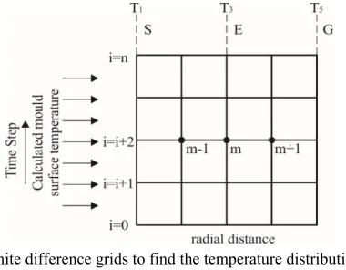
Finite Difference formulation for validation
The calculated mould surface temperature (T1) at particular time interval
was given as input for the direct heat conduction problem. The temperature distribution at different nodes from point S to G is calculated by FDM technique for the given surface temperature (T1) as shown in
figure (4). These calculated temperature at location G in the direct region were used to validate the results of control volume technique.
The finite difference approximation may be derived using the Taylor series expansion for the 1 D transient heat conduction problem for the derivatives 𝜕𝜕𝜕𝜕𝜕𝜕2𝑇𝑇2, 𝜕𝜕𝑇𝑇𝜕𝜕𝑑𝑑in the equation (2). The dependent variable values in a transient heat conduction problem for the future time steps were evaluated from the known set of initial conditions using explicit method. The values of temperature available at the current time step‘t’ was denoted by the superscript ‘i’ as 𝑇𝑇𝑚𝑚𝑖𝑖 . The next calculated temperature
values for the next time step‘t+∆t’ was represented by the superscript ‘i+1’ as𝑇𝑇𝑚𝑚𝑖𝑖+1 is given in Fig.4.
Fig. 4 Finite difference grids to find the temperature distribution in the mould for DHCP
The finite difference grid points for the estimation of the next time step temperature distribution in the mould is given in equation (15):
𝑇𝑇𝑚𝑚𝑖𝑖+1= (1−2𝐹𝐹𝐹𝐹)𝑇𝑇𝑚𝑚𝑖𝑖 +�𝐹𝐹𝐹𝐹 �1−∆𝜕𝜕𝜕𝜕
𝑖𝑖�� 𝑇𝑇𝑚𝑚−1
𝑖𝑖 +𝐹𝐹𝐹𝐹 �1 +∆𝜕𝜕
𝜕𝜕𝑖𝑖� 𝑇𝑇𝑚𝑚+1
𝑖𝑖 (15)
5 The calculated temperature using the equation (15) was compared with the temperature measured at the same node (G) as described in the flow chart for validation of results in Fig.5.
5.
R
ESULTS AND DISCUSSION5.1
Experimental cooling curves
Fig.6 shows the variation of temperature with respect to time recorded by a thermocouples located in the cast (Tc) and in the mould at 20 mm,
30 mm, and 40 mm respectively. The temperature readings were recorded until the difference between the cast temperature and the mould temperature is considerably less. The cast temperature measured by thermocouple Tc suddenly increases after pouring and reaches a maximum value of 655ºC after 22 sec and then decreases gradually as shown. From the graph it is observed that the maximum temperature recorded by a thermocouple located at 10 mm from mould surface is 544.5ºC after 65 sec from pouring and reduced as time increases. The maximum temperature attained by the mould at this location was mainly due to the high latent heat release, high thermal conductivity of aluminum cast and also the position of thermocouple.
Fig. 6 Experimental transient cooling curves
5.2 Calculated mould surface temperature, heat flux and IHTC
The mould surface temperature calculated using inverse control volume technique with respect to time is shown in Fig. 7. From the graph it is observed that the mould surface temperature increased to a maximum value of 508ºC in a short duration of 34 sec and then suddenly drops to 200ºC at 106 sec. This sudden drop in temperature is due to large difference in temperature between the solidifying cast and sand mould. Thereafter the decrease in mould surface temperature is gradual and reaches approximately 100ºC at 180 sec. This is due to high thermal inertia of the moulding sand. Beyond this, the mould surface temperature is almost constant.
Fig. 7 Mould surface temperature with respect to time
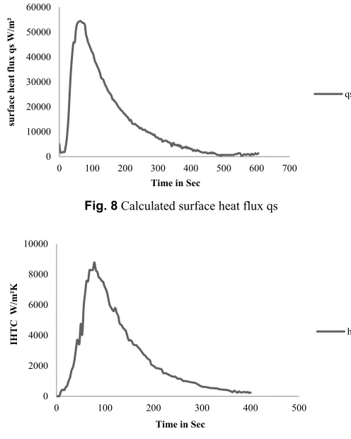
The calculated heat flux at the mould surface is shown in Fig.8. The trend of calculated heat flux is same as that of mould surface temperature. The maximum value is found to be 55,000 W/m2 at 35 sec and decreases
gradually and reaches a value of 3000 W/m2 in 400 sec.
Fig. 8 Calculated surface heat flux qs
Fig. 9 Calculated interfacial heat transfer coefficient
Fig. 10 IHTC variation with cast surface temperature
The variations of IHTC with respect to time and cast surface temperature are shown in Fig.9 and Fig.10. From the figures it is clear that the IHTC reaches peak value of 8870 W/m2K immediately after
pouring. This is due to more contact of the metal with the mould surface at the initial stage. The value of IHTC decreases gradually reaches to value of 1335 W/m2K at 250 sec. The gradual decrease in IHTC is due
to the increase in gap between the solidifying metal and mould due to shrinkage as well the presence of gases in the gap. Thereafter the IHTC gradually decreases and almost maintain a constant trend after 375 sec. This shows that the solidification process is almost completed and there is no change in the properties interfacial of the region.
0 100 200 300 400 500 600 700
0 100 200 300 400 500 600
Te
m
pe
ra
tu
re
in
°C
Time in Sec
Tc T2 T3 T4 T5
0 100 200 300 400 500 600
0 100 200 300 400 500 600
te
m
pe
ra
tu
re
in
⁰C
Time in Sec
0 10000 20000 30000 40000 50000 60000
0 100 200 300 400 500 600 700
su
rf
ac
e h
eat
flu
x q
s W
/m
²
Time in Sec
qs
0 2000 4000 6000 8000 10000
0 100 200 300 400 500
IHTC
W/
m
²K
Time in Sec
h
0 1000 2000 3000 4000 5000 6000 7000 8000 9000 10000
400 450 500 550 600 650 700
IHTC
in
W
/ m
²K
5.3
Validation
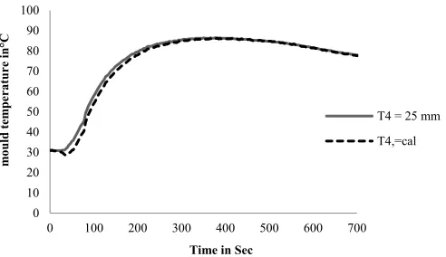
The main objective of the present work is to validate the estimated value of mould temperature by comparing with the experimentally measured temperature data. The estimated mould surface temperature was given as input for the direct heat conduction problem and the temperature history was calculated at various location of the mould. The nodal points were chosen in such a way that any one measured temperatures coincide with the nodal point G (Fig.3). Finite difference method is used to estimate the temperature history.
The estimated temperature at known location (T5) was compared
with the measured temperature data available. Fig.11 shows the comparison of the measured and calculated temperature at location G (T5). It was confirmed from the figure that the calculated temperature
were in good agreement with the measured temperature data. This showed that the accuracy of control volume technique is good as compared to other techniques for the estimation of IHTC by Rajaraman (Rajaraman et al., 2008, 2018).
Fig. 11 Comparison of measured and calculated temperatures at 35 mm from mould surface
6.
C
ONCLUSIONThe following conclusion were arrived in the present work
• The IHTC is calculated between aluminum alloy and sand mould using inverse control volume technique
• The IHTC calculated has a peak value 8870 W/m2K at 80 sec
and then gradually decreases to 1335 W/m2K at 250 sec • The calculated mould temperature is validated by using direct
heat conduction problem and obtained temperature history.
• The estimated and the measured temperature are in good agreement and this testifies to the better accuracy of the selected control volume approach.
NOMENCLATURE
∆r control volume thickness in r direction (m) A heat flow area (m2)
c specific heat (J/kg°C) Fo Fourier number
h interfacial heat transfer coefficient (W/m2°C)
k thermal conductivity (W/m°C) Q heat flow (W)
q heat flux (W/m2)
T temperature (°C) t time (s) Greek symbols
α thermal diffusivity (m2/s)
ρ density (kg/m3)
Superscripts i time step
n total number of future time steps
Subscripts c cast
E thermocouple location at the mould in the inverse region F thermocouple location at the mould in the direct region m nodal point considered
ini initial m mould meas measured cal calculated m mould surface
S location at the mould surface
Abbreviation
IHTC Interfacial Heat transfer coefficient IHCP Inverse heat conduction problem DHCP Direct heat conduction problem FDM Finite Difference method DAQ Data Acquisition system
REFERENCES
Bazhenov, V.E., Koltygin, A.V., Tselovalnik Yu and Sannikov, A.V., 2017, “Determination of Interface Heat Transfer Coefficient between Aluminum Casting and Graphite Mold”, Russian Journal of Non-Ferrous Metals, 58 (2), 114–123.
https://doi.org/10.3103/S1067821217020031
Haci Mehmet Sahin,Kadir Kocatepe, Amazan Kayikci .R. and Nest Akar, 2006, “Determination of unidirectional heat transfer coefficient during unsteady- state solidification at metal casting-chill interface ,” J. of Energy conversion and Management, 47, 19-34.
https://doi.org/10.1016/j.enconman.2005.03.021
Hallam, C.P., and Griffiths W.D, 2004, “A Model of the Interfacial Heat-Transfer Coefficient for the Aluminum Gravity Die-Casting Process”, Metallurgical and Materials Transactions,35B, 721 -733,
https://doi.org/10.1007/s11663-004-0012-x
Hamasaiid, A., Dour, G., Dargusch, M.S., Loulou, T., Davidson, C., and Savage, G., 2008, “Heat-Transfer Coefficient and in-Cavity pressure at the casting-die interface during high-pressure die casting of the Magnesium alloy AZ91D”, Metallurgical and Materials Transactions A,
39A, 853-864.
https://doi.org/10.1007/s11661-007-9452-7.
Jose Eduardo, Spinelli, IvaldoLeao Ferreira and AmauriGarci, 2006, “Evaluation of heat transfer coefficients during upward and downward transient directional solidification of Al–Si alloys”, Struct Multidisc Optim., 31, 241–248.
https://doi.org/10.1007/s00158-005-0562-9
Kovacevic, L., Terek, P., Kakaz, D., and Miletic, A., 2012, “A correlation to describe interfacial heat transfer coefficient during solidification of Al–Si alloy casting”, Journal of Materials Processing,
212, 1856–1861.
https://doi.org/10.1016/j.jmatprotech.2012.04.007
Liqiang Zhang and Luoxing Li, 2013, “Determination of heat transfer coefficients at metal/chill interface in the casting solidification process”, Heat Mass Transfer,49, 1071–1080.
https://doi.org/10.1007/s00231-013-1147-6
0 10 20 30 40 50 60 70 80 90 100
0 100 200 300 400 500 600 700
m
ou
ld
te
m
pe
ra
tu
re
in
°C
Time in Sec
7 Liqiang Zhang, Carl Reilly, Luoxing Li, Steve Cockcroft and Lu Yao, 2014, “Development of an inverse heat conduction model and its application to determination of heat transfer coefficient during casting solidification”, Heat and Mass Transfer, 50 (7) , 945–955.
https://doi.org/10.1007/s00231-014-1304-6
Rajaraman, R., and Velraj, R., 2008, “Comparison of interfacial heat transfer coefficient estimated by two different techniques during solidification of cylindrical aluminum alloy casting” Journal of Heat and Mass transfer, 44, 1025-1034.
http://dx.doi.org/10.1007/s00231-007-0335-7
Rajaraman, R., Anna Gowsalya, L., and Velraj, R.., 2018, “Interfacial heat transfer coefficient estimation during solidification of rectangular aluminum alloy casting using two different inverse methods” Frontiers in Heat and Mass Transfer (FHMT), 11, 23.
http://doi:10.5098/hmt.11.23
Ranjbar, A., A., Ezzati, M., and Famouri, M., 2009, “Optimization of experimental design for an inverse estimation of the metal-mold heat transfer coefficient in the solidification of Sn-10% Pb,” Journal of Materials Processing Technology, 209, 5611-5617.
https://doi.org/10.1016/j.jmatprotec.2009.05.019
Xuezhi Zhang, Li Fang, Zhizhong Sun, Henry Hu, Xueyuan Nie and Jimi Tjong, 2016, “Interfacial heat transfer in squeeze casting of magnesium alloy AM60 with variation of applied pressures and casting wall-thicknesses”, Heat Mass Transfer,52, 2303–2315.
https://doi.org/10.1007/s00231-015-1744-7
Yiwei Dong, Kun Bu, Yangqing Dou and Dinghua Zhang, 2011, “Determination of interfacial heat-transfer coefficient during investment-casting process of single-crystal blades” Journal of Materials Processing Technology, 211, 2123– 2131.
https://doi.org/10.1016/j.jmatprotec.2011.07.012
Howard, E., Boyer, and Timothy, L., Gall, Eds., Metals Hand Book, 1985, American Society for Metal, Materials Park, OH.
Krzysztof Grysa, 2011, “Inverse Heat Conduction Problems, Heat Conduction - Basic Research”, ISBN: 978-953-307-404-7, In. Tech.
Necati Ozisik, M., Helcio, R., and Orlande, B., 2000, “Inverse Heat Transfer Fundamentals and Applications”, Taylor & Francis.
Veerarajan, T., and Ramachandran, T., 2004, “Theory and problems in numerical methods with programs in C and C++”, Tata McGraw-Hill