Journal of Information Technology and Computer Science Volume 3, Number 1, 2018, pp. 1-15
Journal Homepage: www.jitecs.ub.ac.id
Introducing a Practical Educational Tool for Correlating
Algorithm Time Complexity with Real Program Execution
Gisela Kurniawati1, Oscar Karnalim2
Maranatha Christian University, Prof. Drg. Surya Sumantri Street No.65, Bandung, West Java, 40164, Indonesia
[email protected], [email protected]
Received 30 January 2018; accepted 08 June 2018
Abstract. Algorithm time complexity is an important topic to be learned for programmer; it could define whether an algorithm is practical to be used on real environment or not. However, learning such material is not a trivial task. Based on our informal observation regarding students’ test, most of them could not correlate Big-O equation to real program execution. This paper proposes J-CEL, an educational tool that acts as a supportive tool for learning algorithm time complexity. Using this tool, user could learn how to correlate Big-O equation with real program execution through intuitive graphics (resulted from providing three components: Java source code, source code input set, and time complexity equations). According to our evaluation, students feel that J-CEL is helpful for learning the correlation between Big-O equation and real program execution. Further, the use of Pearson correlation in J-CEL shows a promising result.
1
Introduction
Algorithm time complexity indicates how fast an algorithm runs in regard to input size [1]. It is an important topic to be learned for programmer; it could define whether an algorithm is practical to be used on real environment. Therefore, it is listed as a required topic to be mastered for undergraduates in Computer Science (CS) curricula [2].
At CS undergraduate major, algorithm time complexity is usually taught theoretically using Big-O notation; where operations on given algorithm are correlated to input size through abstracted pseudo-execution. It is true that such notation is helpful for learning time complexity. However, according to our informal observation, some students find it difficult to correlate Big-O equation to real program execution. They need some real examples regarding to that correlation.
2
Related Works
In general, despite various terminologies used, Computer Science (CS) educational tool can be classified into twofold: programming-oriented and algorithm-oriented educational tool [3, 5].
Programming-oriented educational tool puts more stress on technical knowledge such as how to write a program. At CS undergraduate major, it has been frequently used for learning Introductory Programming; such tool is proved to be effective for teaching undergraduate students [6–9]. Most programming-oriented educational tools are either program visualization or visual programming tool. On the one hand, program visualization tool is focused on simulating how a program works. It is usually featured with a rich information regarding running program (e.g., variable state). Several examples of program visualization tool are PythonTutor [10], OmniCode [11], SRec [12], Jelliot 3 [13], JIVE [14], and VILLE [15]. On the other hand, visual programming tool is focused on preventing errors caused by writing the code directly. It is usually featured with indirect interaction mechanism between user and target program. Several examples of visual programming tool are Raptor [16], SFC Editor [17], Scratch [18], Alice [19] and Greenfoot [20].
Algorithm-oriented educational tool puts more stress on algorithmic steps. At CS undergraduate major, it has been frequently used to cover complex topic such as data structures [21, 22] and algorithm strategies [3, 23–26]. When perceived from how they focus on visualization, algorithm-oriented educational tools can be further classified into twofold: algorithm visualization and standard algorithm-oriented educational tool. On the one hand, algorithm visualization tool focuses on utilizing visualization as its main interaction feature. Different with program visualization tool, it involves no specific programming language. In other words, it displays more abstract information than program visualization tool. Several examples of such tool are VisuAlgo [22], AP-ASD1 [21], AP-SA [23], and AP-BB [24]. On the other hand, standard algorithm-oriented educational tool does not focus on visualization as its main feature. Several examples of such tool are GreedEx [26], GreedExCol [25], and Complexitor [3].
Algorithm time complexity is a metric used to measure the time growth of a particular algorithm toward input size [1]. In other words, it could be used to define whether a particular algorithm is practical to be used on real environment. Despite its benefit, learning algorithm time complexity is not a trivial task. According to our informal observation regarding students’ test toward that topic, most of them could not grasp the idea behind calculating algorithm time complexity using Big-O notation. They could not correlate Big-O equation to real program execution. Further, an informal survey provided by [3] also shows similar phenomenon.
Kurniawati, G. et al. Introducing a Practical Educational Tool ... 3
3 Proposed Methodology
This paper proposes an educational tool that acts as a supportive tool for learning algorithm time complexity. It is named J-CEL (Java-based time Complexity Educational tooL). Using this tool, user could learn how to correlate Big-O equation with real program execution by providing three components: arbitrary source code (written in Java programming language), source code input set, and time complexity equations.
It is true that Complexitor [3], at some extent, also aims similar goal as ours. However, we would argue that our proposed tool is more practical to be used in real environment: user is not required to have deep technical knowledge regarding target programming language since programming-language-dependent syntaxes are automatically generated. Further, we also provide richer information regarding time complexities and their respective correlation.
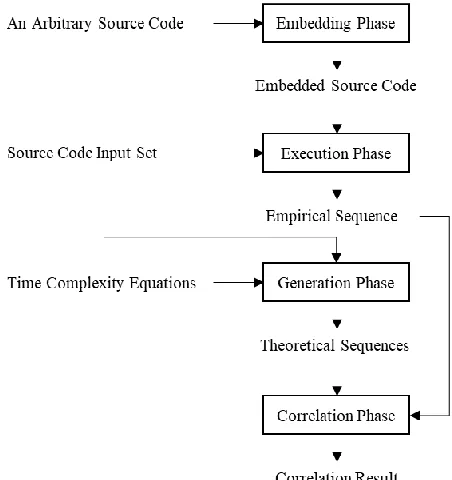
The correlations between time complexity equation and real programming execution are calculated using methodology given on Fig. 1. It contains four phases which are embedding, execution, generation, and correlation phase.
Fig. 1. Proposed methodology to generate the correlations between time complexity equation and real programming execution.
example about that counter mechanism can be seen in [3].
To automatically embed statements, ANTLR [27] is used to parse inputted source code and locate desired positions. Since ANTLR requires different lexer and parser for each programming language, we limit our target programming language to Java as our case study.
Execution phase will generate an empirical sequence (i.e., a sequence that represents the number of process for real program execution) by executing embedded source code multiple times with respect to source code input set. Empirical sequence will be used for correlating time complexity with real program execution at correlation phase. Execution phase works in twofold. At first, embedded source code will be compiled to a program. Later, each input stream from source code input set will be fed to given program; each input stream will result an integer representing the number of process toward given stream. These integers will be sorted based on input size in ascending order and returned as an empirical sequence.
Generation phase will generate theoretical sequences with respect to the number of time complexity equations. Each equation will result one theoretical sequence where each integer on given sequence represents the number of process for given complexity toward given input. Theoretical sequences will be used for correlating time complexity with real program execution at correlation phase.
Correlation phase will generate correlation value for each theoretical sequence toward empirical sequence. It will be calculated using Pearson correlation algorithm [4], a well-known algorithm to correlate two sequences. Since the correlation between two constant sequences cannot be detected through Pearson correlation, the correlation between constant theoretical sequence (i.e., O(1))and empirical sequence will be calculated by measuring how far the difference between each empirical value and the mean of empirical values. If all differences are lower than 10% of the mean, that empirical sequence will be assumed as constant sequence with 1 as its correlation value. This mechanism is adopted from [3].
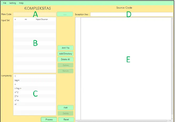
To enhance user understanding further, J-CEL is featured with two intuitive User Interfaces (UIs). The first UI will be used to accept three input components while the second one will be used to display resulted correlations.
Kurniawati, G. et al. Introducing a Practical Educational Tool ... 5
code.
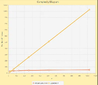
J-CEL’s UI for displaying correlation result can be seen on Fig. 4. It contains four panels which are graph setting panel, correlation graph display, input stream selection panel, and source code display. These panels are referred as A, B, C, and D respectively on Fig. 4.
First, graph setting panel is used to manipulate correlation graph display. User can select which time complexity equation he wants to display. Further, he can also set how many logarithmic layers that will be applied to given graph. Logarithmic layer is used to mitigate the gap between theoretical and empirical sequence when such difference cannot be seen by default: applying logarithmic layer will reduce the difference between two numbers while keeping their comparison order similar (see Fig. 5 for an example about applying a logarithmic layer to a graph displayed on Fig. 4). To provide clearer analysis for users, J-CEL is also featured with a default prediction of time complexity on graph setting panel. It will show time complexity equation which correlation toward empirical sequence is the highest.
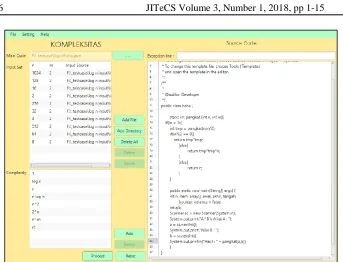
Fig. 3. J-CEL’s UI for accepting input components when all components are ready.
Kurniawati, G. et al. Introducing a Practical Educational Tool ... 7
Fig. 5. Correlation graph display from Fig. 4 that has been applied with a logarithmic layer.
Second, correlation graph display is used to show how close the correlation between selected theoretical sequence and the empirical one. Each sequence will be represented with a line; orange line refers to theoretical sequence while the red one refers to empirical sequence. On given display, horizontal axis represents input size while vertical axis represents the number of process; similar line equation refers to high correlation between theoretical and empirical sequence (see Fig. 4 for an example of high correlation and Fig. 6 for an example of low correlation). It is important to note that resulted display will rely on inputs given on graph setting panel. If log layer(s) is applied, displayed graph will be automatically changed with more stress on slight difference between given sequences.
Third, input stream selection panel is used to manipulate the number of process on source code display. User can select which input stream he wants to relate with the number of process. In addition, user can also see the detail of input stream and check resulted output from executing targeted source code with given input. He is only required to press related buttons.
Fourth, source code display is used to display the relation between source code statements and their respective number of process. Such relation is displayed to provide further understanding toward the correlation between time complexity and empirical execution. The number of process for each statement is resulted from actual execution of given source code toward predefined input stream. Moreover, the total of all numbers of process is also provided at the bottom of source code display.
4 Evaluation
Five evaluation schemes are conducted: black-box evaluation, questionnaire-based evaluation, evaluation regarding minimum number of input stream, evaluation regarding non-asymptotic Big-O equation, and evaluation regarding the impact of involved statements. The first two schemes are related to J-CEL’s usability while the others are related to the characteristics of Pearson correlation for connecting theoretical sequence to empirical one.
4.1 Black-Box Evaluation
This evaluation scheme validates features provided by J-CEL. For each feature, its functionality is checked by simulating how user would use such feature. According to our findings, all J-CEL’s features work correctly as expected. They generate no error during the simulation.
4.2 Questionnaire-based Evaluation
This evaluation scheme validates whether J-CEL helps student for learning the correlation between Big-O equation and real program execution. Questionnaire surveys were distributed to 23 undergraduate students which had taken Algorithm Strategy course (i.e., a course where one of its topic is about algorithm time complexity) at our major. Each of them should rate 8 statements regarding to the use of J-CEL (see Table 1 for the detail of statements) in 4-points Likert scale (1 refers to strongly disagree, 2 refers to weakly disagree, 3 refers to weakly agree, and 4 refers to strongly agree). Further, rationale for the rating of each statement is also asked to be provided. To generate more objective result, these students had been asked to use J-CEL before they filled the survey.
Kurniawati, G. et al. Introducing a Practical Educational Tool ... 9
clear enough to see the correlation between theoretical and empirical sequence in detail.
Table 1. Statements in Questionnaire Survey
ID Statement
S1 Time complexity prediction on graph setting panel helps student to know time complexity of a particular algorithm,
S2 Correlation graph display helps student to correlate theoretical sequence with empirical one.
S3 Correlation graph display helps student to determine which theoretical sequence is the most correlated one toward given empirical sequence.
S4 The number of process resulted for each input stream helps student to understand which statements generate slow or fast processing time.
S5 The existence of logarithmic layer helps student to see the correlation between theoretical and empirical sequence in detail.
S6 J-CEL helps student to get a brief insight about the impact of time complexity. S7 A mechanism to add time complexity equation helps student to understand the correlation between Big-O notation and real program execution through trial and error.
S8 Exception line helps student to only consider core operations for correlating Big-O notation and real program execution.
Fig. 7. Mean and standard deviation of questionnaire survey result.
theoretical and empirical sequence. Fourth, S7 is weakly disagreed by two respondents. One of them stated that it is unclear about how to perform trial and error while another one stated that it is hard to write Big-O notation through given mechanism. Last, S8 is weakly disagreed by one respondent. He stated that it is impractical to put exception lines manually. It is important to note that, since the number of weakly-disagree rating is low, these rationales will be considered further on future work.
4.3 Evaluation regarding Minimum Number of Input Stream
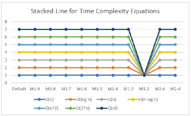
This evaluation scheme enlists minimum number of input stream required for each well-known asymptotic algorithm time complexity. There are 7 time complexity equations involved: O(1), O(log n), O(n), O(n log n), O(n2), O(2n), and O(n!). Each equation will be featured with a source code that generates such complexity and ten input streams with various input sizes. The first five equations will use input size with 2t growth and the last two equations will use input size with t growth. t refers to positive integer starting from 1 to 10. In other words, the first five equations will involve 2, 4, 8, 16, 32, 64, 128, 256, 512, and 1024 as their input sizes while the last two equations will involve 1, 2, 3, 4, 5, 6, 7, 8, 9, and 10 as their input sizes.
To evaluate minimum number of input stream, eleven evaluation schemes for each time complexity equation will be generated. One of them is generated by involving all input sizes, eight of them will be generated by iteratively removing the largest input size, and the other two will be generated by iteratively excluding in-between input sizes (i.e., input sizes that are placed at neither the beginning nor the end of the list). The latter mechanism is proposed to check whether the range between input sizes affects resulted correlation.
To provide clearer view about proposed mechanisms to generate evaluation schemes, suppose we have ten input streams with 2, 4, 8, 16, 32, 64, 128, 256, 512, and 1024 as their respective input size. Input sizes for each evaluation scheme can be seen in Table 2. The name for each scenario except default is prefixed with either M1 (for a mechanism that removes the largest input size) or M2 (for another mechanism). Such name is then followed by a positive integer representing the number of input stream. As seen in Table 2, it is clear that M1 excludes the largest input size each time its new scenario is generated. Further, M2 excludes input size in position 2, 5, 6, & 9 from default to generate M2-6 and excludes input size in position 2 & 5 from M2-6 to generate M2-4.
Minimum number of input stream for each time complexity equation is evaluated by executing its respective source code toward input streams provided by aforementioned scenarios and checking which scenario with the fewest input streams generates the highest correlation for correct time complexity equation. The result of that evaluation can be seen on Fig. 8. All equations are assigned correctly with the highest correlation on most scenarios. These equations except O(1) are only assigned incorrectly on M1-2. We would argue that such finding is natural considering the number of input stream on such scenario is limited and these input streams are only slightly different to each other. Pearson correlation could not distinguish correct equation among the wrong ones on those conditions. It is important to note that O(1)
Kurniawati, G. et al. Introducing a Practical Educational Tool ... 11
Table 2. The Examples of Involved Input Sizes for Evaluation Schemes
Mechanism Involved Input Sizes
Default 2, 4, 8, 16, 32, 64, 128, 256, 512, 1024 M1-9 2, 4, 8, 16, 32, 64, 128, 256, 512 M1-8 2, 4, 8, 16, 32, 64, 128, 256 M1-7 2, 4, 8, 16, 32, 64, 128 M1-6 2, 4, 8, 16, 32, 64 M1-5 2, 4, 8, 16, 32 M1-4 2, 4, 8, 16 M1-3 2, 4, 8 M1-2 2, 4
M2-6 2, 8, 16, 128, 256, 1024 M2-4 2, 16, 128, 1024
As seen in Fig. 8, scenarios generated by both M1 and M2 are favorable for each equation except when the number of input stream is 2. Hence, it can be stated that the range between input size does not affect correlation result and generated correlation result will be correct as long as its number of input stream is higher than 2 with reasonable range between input streams (in our case, we assign 2t growth for low time complexity equations and t growth for high time complexity equations where t refers to positive integer).
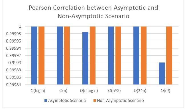
4.4 Evaluation regarding Non-Asymptotic Big-O Equation
This evaluation scheme validates whether resulted Pearson correlation is increased when asymptotic Big-O equation is incorporated and the difference between non-asymptotic and non-asymptotic equation is considerably large. To do so, time complexity equations defined for evaluating the minimum number of input stream except O(1)
will be used. O(1) is excluded since determining such complexity does not require Pearson correlation. For each equation, two scenarios are proposed: asymptotic and non-asymptotic scenario. The former one refers to a condition where inputted equation is the non-asymptotic one while the latter one refers to a condition where inputted equation is the asymptotic one. It is important to note that non-asymptotic scenario is implemented by utilizing J-CEL’s feature to add new time complexity equation.
Pearson correlation result for both scenario toward all involved time complexity equations can be seen in Fig. 9. Non-asymptotic scenario generates higher or similar correlation value when compared to the asymptotic one. We would argue that similar correlation value between both scenarios on several equations is natural considering the difference between equation used in both scenarios is extremely small. Consequently, it still can be stated that resulted Pearson correlation is increased when asymptotic Big-O equation is incorporated and the difference between non-asymptotic and non-asymptotic equation is considerably large.
Fig. 9. Pearson correlation between asymptotic and non-asymptotic scenario for each equation. The highest possible correlation for each scenario is 1.
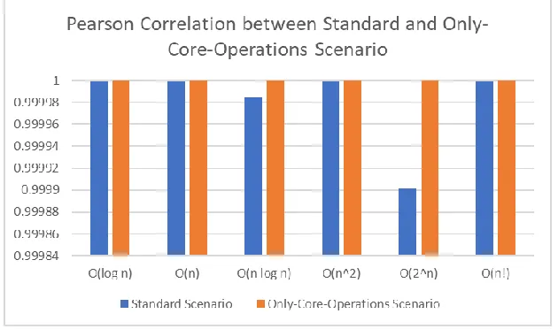
4.5 Evaluation regarding The Impact of Involved Statements
This evaluation scheme validates whether resulted Pearson correlation is increased when only statements related to core operations are involved. Time complexity equations defined for evaluating the minimum number of input stream except O(1)
Kurniawati, G. et al. Introducing a Practical Educational Tool ... 13
involved while the latter one refers to a condition where only statements related to core operations are involved. Only-core-operations scenario is implemented by utilizing J-CEL’s exception lines.
Pearson correlation result for both scenarios toward all involved time complexity equations can be seen in Fig. 10. Only-core-operations scenario generates higher correlation value when compared to the standard one. Such finding is natural since only-core-operations scenario excludes input and output statements from each case, resulting more accurate empirical sequence. Hence, it can be stated that resulted Pearson correlation is increased when only statements related to main operations are involved.
Fig. 10. Pearson correlation between standard and only-core-operations scenario for each equation. The highest possible correlation for each scenario is 1.
5 Conclusion and Future Work
References
1. Levitin, A.: Introduction to the design & analysis of algorithms. Pearson (2012).
2. on Computing Curricula, A. for C.M. (ACM), Society, I.C.: Computer Science Curricula 2013: Curriculum Guidelines for Undergraduate Degree Programs in Computer Science. ACM, New York, NY, USA (2013).
3. Elvina, E., Karnalim, O.: Complexitor: An Educational Tool for Learning Algorithm Time Complexity in Practical Manner. ComTech: Computer, Mathematics and Engineering Applications. 8, 21 (2017).
4. Pearson, K.: Note on Regression and Inheritance in the Case of Two Parents.
5. Sorva, J., Karavirta, V., Malmi, L.: A Review of Generic Program Visualization Systems for Introductory Programming Education. ACM Transactions on Computing Education. 13, 1–64 (2013).
6. Kaila, E., Rajala, T., Laakso, M.J., Salakoski, T.: Effects of Course-Long Use of a Program Visualization Tool. In: Australasian Computing Education Conference. , Brisbane (2010). 7. Karnalim, O., Ayub, M.: The Effectiveness of a Program Visualization Tool on
Introductory Programming: A Case Study with PythonTutor. CommIT (Communication and Information Technology) Journal. 11, (2017).
8. Karnalim, O., Ayub, M.: The Use of PythonTutor on Programming Laboratory Session: Student Perspectives. KINETIK. 2, (2017).
9. Cisar, S.M., Pinter, R., Radosav, D.: Effectiveness of Program Visualization in Learning Java: a Case Study with Jeliot 3. International Journal of Computers, Communications & Control. 6, (2011).
10. Guo, P.J.: Online python tutor: embeddable web-based program visualization for cs education. In: Proceeding of the 44th ACM technical symposium on Computer science education - SIGCSE ’13. p. 579. ACM Press, New York, New York, USA (2013).
11. Kang, H., Guo, P.J.: Omnicode: A Novice-Oriented Live Programming Environment with Always-On Run-Time Value Visualizations. In: The 30th ACM Symposium on User Interface Software and Technology (UIST (2017).
12. Velázquez-Iturbide, J.Á., Pérez-Carrasco, A., Urquiza-Fuentes, J.: SRec: : an animation system of recursion for algorithm courses. In: Proceedings of the 13th annual conference on Innovation and technology in computer science education - ITiCSE ’08. p. 225. ACM Press, New York, New York, USA (2008).
13. Moreno, A., Myller, N., Sutinen, E., Ben-Ari, M.: Visualizing programs with Jeliot 3. In: Proceedings of the working conference on Advanced visual interfaces - AVI ’04. p. 373. ACM Press, New York, New York, USA (2004).
14. Gestwicki, P., Jayaraman, B.: Interactive Visualization of Java Programs. In: Symposia on Human Centric Computing Languages and Environments (2002).
15. Rajala, T., Laakso, M.-J., Kalla, E., Salakoski, T.: VILLE: a language-independent program visualization tool. In: Proceedings of the Seventh Baltic Sea Conference on Computing Education Research - Volume 88. pp. 151–159. Australian Computer Society, Darlinghurst (2007).
16. Carlisle, M.C., Wilson, T.A., Humphries, J.W., Hadfield, S.M.: RAPTOR: a visual programming environment for teaching algorithmic problem solving. Acm Sigcse Bulletin. 37, 176–180 (2005).
17. Watts, T.: The SFC editor a graphical tool for algorithm development. Journal of Computing Sciences in Colleges. 20, 73–85 (2004).
Kurniawati, G. et al. Introducing a Practical Educational Tool ... 15
Eastmond, E., Brennan, K., Millner, A., Rosenbaum, E., Silver, J.: Scratch: Programming for All. Communications of the ACM. 52, 60 (2009).
19. Cooper, S., Dann, W., Pausch, R.: Alice: a 3-D tool for introductory programming concepts. In: Journal of Computing Sciences in Colleges. pp. 107–116 (2000).
20. Kölling, M.: The greenfoot programming environment. ACM Transactions on Computing Education (TOCE). 10, 14 (2010).
21. Christiawan, L., Karnalim, O.: AP-ASD1 : An Indonesian Desktop-based Educational Tool for Basic Data Structure Course. Jurnal Teknik Informatika dan Sistem Informasi. 2, (2016).
22. Halim, S., Chun KOH, Z., Bo Huai LOH, V., Halim, F.: Learning Algorithms with Unified and Interactive Web-Based Visualization. Olympiads in Informatics. 6, 53–68 (2012). 23. Jonathan, F.C., Karnalim, O., Ayub, M.: Extending The Effectiveness of Algorithm
Visualization with Performance Comparison through Evaluation-integrated Development. In: Seminar Nasional Aplikasi Teknologi Informasi (SNATI) (2016).
24. Zumaytis, S., Karnalim, O.: Introducing an Educational Tool for Learning Branch & Bound Strategy. Journal of Information Systems Engineering and Business Intelligence. 3, 8 (2017).
25. Debdi, O., Paredes-Velasco, M., Velázquez-Iturbide, J.Á.: GreedExCol, A CSCL tool for experimenting with greedy algorithms. Computer Applications in Engineering Education. 23, 790–804 (2015).
26. Velázquez-Iturbide, J.Á., Pérez-Carrasco, A.: Active learning of greedy algorithms by means of interactive experimentation. In: Proceedings of the 14th annual ACM SIGCSE conference on Innovation and technology in computer science education - ITiCSE ’09. p. 119. ACM Press, New York, New York, USA (2009).
27. Parr, T.: The definitive ANTLR 4 reference. Pragmatic Bookshelf (2013).