Display of the β-effect in the Black Sea Two-Layer Model

Display of the

β-effect in the Black Sea Two-Layer Model

A.A. Pavlushin, N.B. Shapiro, E.N. Mikhailova

Marine Hydrophysical Institute, Russian Academy of Sciences, Sevastopol, Russian Federation e-mail: [email protected]

The research is a continuation of a series of numerical experiments on modeling formation of wind currents and eddies in the Black Sea within the framework of a two-layer eddy-resolving model. The main attention is focused on studying the β-effect role. The stationary cyclonic wind is used as an external forcing and the bottom topography is not considered. It is shown that at the β-effect being taken into account, the Rossby waves propagating from east to west are observed both during the currents’ formation and at the statistical equilibrium mode when the mesoscale eddies are formed. In the integral flows’ field the waves are visually manifested in a form of the alternate large-scale cyclonic gyres and zones in which the meso-scale anti-cyclones are formed. This spatial pattern constantly propagates to the west that differs from the results of calculations using the constant Coriolis parameter when the spatially alternate cyclonic and anti-cyclonic vortices are formed, but hold a quasi-stationary position. The waves with the parameters of the Rossby wave first barotropic mode for the closed basin are most clearly pronounced. Interaction of the Rossby waves with large-scale circulation results in intensification of the of the currents’ hydrodynamic instability and in formation of the mesoscale eddies. Significant decrease of kinetic and available potential energy as compared to the values obtained at the constant Coriolis parameter is also a consequence of the eddy formation intensification.

Keywords: the Black Sea, eddy-resolving model, numerical experiment, β-effect, Rossby waves.

DOI: 10.22449/1573-160X-2016-5-3-23

© 2016, A.A. Pavlushin, N.B. Shapiro, E.N. Mikhailova © 2016, Physical Oceanography

Introduction. To investigate the effect of various factors (internal and external) on the formation and evolution of the hydrophysical fields in the Black Sea, a series of targeted numerical experiments with eddy-resolving two-layer isopycnic model was carried out [1, 2]. The model is based on a system of primitive equations in the Boussinesq, hydrostatic and β-plane approximations. The sea comprising of two layers with the upper layer density ρ₁=const and the lower layer oneρ₂ =const. The layers are not mixed with each other. The friction between the layers can be taken into account in the model. The tangential wind stress τ is set on the sea surface. The energy sink is carried out at the expense of the bottom friction and horizontal turbulent viscosity.

The equations of motion and continuity, vertically integrated within each layer, have the following form

( ) (

) (

)

( )

(

)

( ) (

) (

)

( )

(

)

( ) ( ) ( )

( ) ( ) ( )

, 0 , , 2 2 2 1 1 1 2 2 1 2 2 2 2 2 2 2 2 2 2 1 2 2 2 2 2 2 2 2 = + + = + + ∇ ∇ + − + ′ + = = + + + ∇ ∇ + − + ′ + = − + + y x t y x t l y b y a y y y x t l x b x a x x y x t V U h V U h v h A R R h h g gh fU V v V u V u h A R R h h g gh fV U v U u U ζ ζ (1)

where indices 1 and 2 denote the upper and lower layer correspondingly; the lower indices x, y and t designate differentiation; u_i,v_i are the i-layer horizontal components of the current velocity; h ₁, h₂ are the layer thickness; U1=uihi,

i ih v

V₁ = are the flow components; ζ is the sea level; Rax = ra

(

)

(

)

r

R_ay = _a − are the components of the friction force between the layers;

2 u r

R_bx = _b , Rby =rbv2 are the bottom friction force components; r a, rb are the

constant coefficients; f = f0+βy is the Coriolis parameter,

4 0 10 − = f 1/s, 13 10 2⋅ − =

β 1/(сm∙s); g=980 g∙сm/s2 _{is the free fall acceleration;}

(

)

=

′ g

g ; τx, τy are the tangential wind stress components; Al is the

horizontal eddy viscosity coefficient.

The integral continuity equation in the rigid lid approximation terminates the equations. It permits to introduce the stream function ψ for the total flows:

y

U

U₁+ ₂ =−ψ , V1+V2 =ψx.

At the side basin boundaries the no-slip conditions are set. River runoff into the sea and water exchange through the straits are not taken into account. Initially, the water is at rest, the interface layer and the sea surface are horizontal.

In the finite-difference model representation a time two-layer numerical scheme is applied. It is based on the B-grid box method (in the terminology of Arakawa), the implicit approximation of the Coriolis force and friction forces on the section and the bottom surface. Advective members in the equations of continuity are approximated by the first accuracy order (directed differences) scheme and in the equations of motion – by the second accuracy order scheme of the (Lax – Wendroff).

The paper [1] presents the analysis of the results of experiments with different coefficients of horizontal turbulent viscosity Al and bottom friction rb at the

constant Coriolis parameter f0 = 10-4 1/s, corresponding to the Black Sea latitude. It

is shown that satisfactory results in the model are obtained using the coefficients

Al ~ 105 cm2/s and rb in the range of 0.01 – 0.1 cm/s. Under these parameters in the

basin alongside with the stable quasi-stationary cyclonic gyres the mesoscale anticyclonic eddies associated with the hydrodynamic instabilities of currents sporadically appear.

In the paper [2] the effect of the basin shape on circulation was studied. The results of calculations of current fields in basins with different configurations in the absence of β-effect were analyzed. In the stretched basins, provided the bottom friction is quite weak, the large-scale circulation is divided into individual cyclonic eddies, even without the protruding coastline elements available. The number of these eddies depends on the ratio of the length of the basin to its width.

In the papers [1, 2] the energy inflow in the sea under the stationary wind const

) (t =

τ is also shown to be regulated by the oscillatory process [3] associated with changes in the work of the tangential wind stress W_τ =τ⋅u₁ ⋅cos(α). This is

due to the transformation of the surface current field u1 

by mesoscale eddies generated by hydrodynamic (barotropic and/or baroclinic) large-scale circulation instability. The period of oscillation in the β-effect absence is mainly determined by the lifetime of mesoscale eddies.

In the present article the research of the β-effect role on the formation of wind-driven circulation in the Black Sea is carried out. According to the theory [4 – 6] latitude change of the Coriolis parameter leads to appearance of the planetary Rossby waves, which can have a very wide range of manifestations depending on various conditions. The Black Sea specificity is that it is almost a closed basin. Its size is less than the barotropic (external) Rossby deformation radius, but more than baroclinic (internal) deformation radius.

There are a number of works that are directly or indirectly related to the modeling and description of processes in the Black Sea, connected with the manifestation of planetary waves [7 – 14]. First of all, the works of E. Stanev, N. Rachev [7, 8] should be paid attention to. There the analysis of the numerical simulation of wind circulation in the Black Sea applying the level eddy-resolving Bryan – Cox model is described. The movement in the sea as well as in our case was excited by stationary wind. As a result of computations performed in the Black Sea long-term fluctuations were obtained. They were described as barotropic Rossby waves generated in a closed basin, whose dimensions are smaller than the outer radius of deformation. According to the authors of [8], the Rossby waves are the dominant form of wave motion in the Black Sea and the variability of the circulation associated with planetary modes can be compared in some cases with the variability caused by baroclinic instability.

out on a quasi-periodic mode with the oscillations in the total flow fields with periods of 43 and 83 days. According to opinion of the authors, the first of these periods is associated with the manifestation of baroclinic instability of the main current, and the second one can be caused by manifestation of barotropic Rossby waves.

In [10] based on the processing of satellite observations of the Black Sea level changes the long-period oscillations propagating in the western direction were monitored. The authors explain this process by radiation of the baroclinic Rossby waves, caused by seasonal fluctuations of the wind vorticity from, the eastern coast of the sea.

In [11] based on the analysis of hydrophysical and morphometric characteristics of the Black Sea, the conclusion about the possible existence of the Rossby waves in the basin with periods of 80 – 200 days and phase velocities of 2 – 8 cm/s is drawn.

As the observational data indicating the presence of planetary waves in the Black Sea basin, the works [12, 13] can also be mentioned. They describe the anticyclonic mesoscale eddies generated in the Black Sea during summer. Monitoring of the eddies showed that during the observation period, they had a velocity component of ~ 2 km/day, directed to the west, which may indicate their relation to the Rossby waves.

Generally, the features of the appearance and propagation of planetary waves in the Black Sea have not been studied enough.

Description of the experiments. As it was previously mentioned, the experiments considered in the present paper, are devoted to β-effect and its effect on the formation of wind circulation in the Black Sea. The experiments do not take into account the bottom topography and friction between the layers. τ wind power

is set stationary at a constant cyclonic vorticity 0,5⋅10−7N/m3_{. The sea depth is set}

equal to H = 2200 m. The upper layer initial thickness is h0 = 175 m, the Coriolis

parameter on the southern boundary is β = 2∙10-13 _s-1с_m-1_{, the Rossby parameter is}

β = 2∙10-13 _s-1с_m-1_{, horizontal eddy viscosity coefficient is A}

l = 105 сm2s-1.

In previous studies [1, 2] it was shown that the results of solving the problem under the constant Coriolis parameter are very sensitive to the value of bottom friction, while rb ratio variation range is quite wide. Therefore, computations with

different values of the rb coefficient were carried out.

For the convenience of description, in the present paper we introduced the following alphanumeric designations of the experiments. In the numerical experiments, indicated by the letter B, β > 0, experiments with β = 0 are indicated by the letter A. The paper discusses the results of six experiments: B1, B2, B3 and A1, A2, A3. In addition to β-parameter, the difference between them is in the use of different values of the rb bottom friction coefficient: in B1, A1, B3, A3

experiments rb = 0.01 cm/s; B2, A2 ones – rb = 0.1cm/s.

configuration. This makes it possible to demonstrate the influence of the effect of the basin configuration and coastline features on the formation of currents, eddies and Rossbi waves.

The computations were performed on a 3 × 3 km square grid with a time step of Δt = 3 min. The use of a high spatial resolution compared to the previous works [1, 2], which applied a 4 × 3.5 km grid and time step of Δt = 6 min., permitted to obtain the smaller eddies with an increase in their quantity in the study area

Duration of the computations in each experiment was not less than 10 years. The experiment was stopped after the decision came out on a statistically equilibrium mode [2], in which the averaged time characteristics of the model has changed little over time.

Results of the numerical experiments. The performed computations resulted in obtaining instantaneous and averaged over time fields of the upper layer

thickness h1, the sea level

ζ

integrated stream function ψ.

In addition, graphs of the time changes of area averaged values were

constructed. These values were the kinetic energy of the upper and lower layer KE1

KE2, available potential energy DPE and tangential wind stress work Wτ calculated

according to the following formulas

, 2 / )

( 12

2 1 1 1

1 h u v

KE = ρ + ( 22)/2 ,

2 2 2 2

2 h u v

KE = ρ +

, 2 / )

( _{1 0} 2

1g h h

DPE= ρ ′ − W_τ = ρ₁(u₁τx+v₁τy) ,

where h1, h2 are the upper and lower layer thickness; u1, v1, u2 and v2 horizontal

components of the current velocities in the respective layers; g′=g

(

)

τ

x

,

τ

brackets denote averaging over the area.

Results of the computations obtained under β > 0 were compared with results

of the experiments where β-parameter was assumed to be zero.

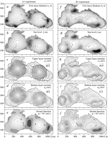
Fig. 1 shows the instantaneous spatial distributions of the features in В1 and

А1 experiments. А1 experiment (β = 0) is characterized by the presence of all the fields in the two large-scale cyclonic gyres (Fig. 1, а – e). One cycle is located in

the western part of the sea, the other – in the east one. These sub-basin cyclones define large-scale circulation in the basin. Between the cyclones and the coast and

between mesoscale cyclones anticyclonic eddies occasionally appear. They are

clearly visible in the h1,

ζ

and

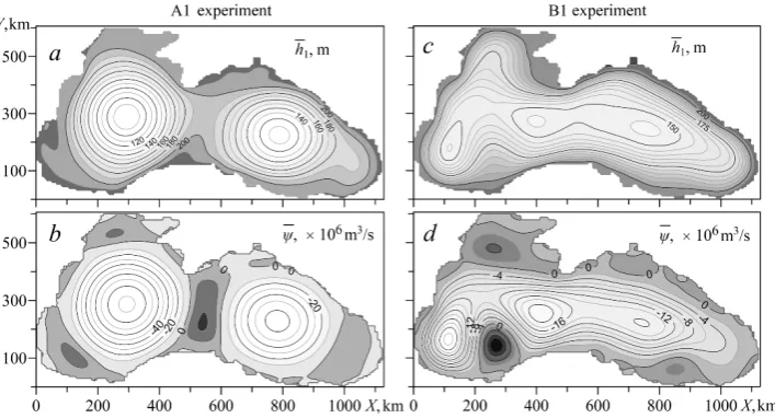
There are clearly distinguished two cyclonic eddies averaged over several in the fields h1 and ψ (Fig. 2, a, b). They were also observed in the instantaneous

distributions. This testifies their stationary nature. With regard to mesoscale

anticyclonic eddies, due to their non-stationarity in time and space, they are weakly manifested in the averaged field ψ and do not appear at all in the field h1.

Fig. 2. Average distributions h1 and ψ in the experiments А1 (left) and В1 (right)

In the experiment (В1) with β-effect taken into account the large-scale cyclones in the sea central part are also found in the instantaneous distributions h1,

ζ and u1 (Fig. 1, а – c) (В1), but, unlike А1 experiment, they are weaker, and their

number is more than two. Therefore, we can rather speak of the presence of a large-scale cyclonic gyre with several peaks in the central part of the given basin. Mesoscale anticyclonic eddies are observed along the coast.

The single cyclonic and anticyclonic eddies are more distinguished in the

fields ψ and u2 _{in B1 experiment than in the upper layer.}

Eddy formations, available in instantaneous fields, are constantly moving. It leads appearance of a vast cyclonic area t in the medium fields h1 and ψ in the

central part of the basin (Fig. 2. c, d). As a consequence of the intensification of western currents, there is a slight thickening of the isolines h1 and ψ near the

western coast.

In both experiments considered the qualitative coincidence of current fields in the upper and lower layers, indicating that the process barotropization is noteworthy. The direction of currents in the upper and lower layers is substantially the same. The velocity of currents in the lower layer is about 40 % of the one in the upper layer.

Integrated stream function ψ, which characterizes the barotropic currents,

correlates well with the fieldu2, and the isolines h1 are close to the current lines

1

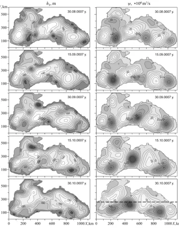
Fig. 3. Consequent fields h1 (left) and ψ (right) with 15 day period in B1 experiment. The dotted line

represents the section Y = 270 km

As it has already been mentioned, the eddy formations occurring under β > 0, do not have a stationary position. If the sequence of instantaneous fields h1 and ψ,

created for B1 experiment, is considered (Fig. 3), the movement of eddy formation has mainly the western direction, which is not observed in A1 experiment.

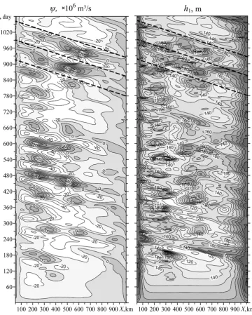
In graphs h1 and ψ (Fig. 4), plotted for the latitudinal section, going through

waves are better manifested than in h1one, as in the upper layer the currents and

mesoscale eddies associated with baroclinic instability are superposed on them.

Fig. 4. Time graphsψ (left) and h1 (right) on the section Y = 270 km in B1 experiment

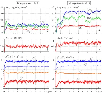
Fig. 5. Energy graphs of KE1, KE2, DPE in В1 (а) and А1 (d) experiments; the tangential wind stress

work Wτ in В1 (b) and А1 (e) experiments; mean vorticity В1 (c) and А1 (f)

Fig. 5 а, d, show the solution reaches a statistically equilibrium mode, the characteristics change within the relatively limited certain mean values in the both experiments.

In В1 experiment under β > 0 the KE1, KE2 and DPE energy values resulted

significantly smaller than in A1 experiment. The work Wτ, which provides the energy inflow in the sea, also appeared smaller. As Wτ is determined by oscillatory process, depending on the stability of currents in the upper layer, it can be assumed that the β-effect influences the currents, making them more instable.

It can be seen if we calculate separately the average area values of cyclonic and anticyclonic relative vorticity in the different layers of the model. It is necessary to sum over areas cyclonic and anticyclonic vorticity values in each layer separately and divide by the corresponding areas. The resulting mean values for cyclonic and anticyclonic vorticity will be denoted asξ₁C, ξ₂C ξ₁Aandξ₂A:

dxdy

y u x v S

i i _C

i i C C

i

∫∫

  

 

∂ ∂ − ∂ ∂

= 1

ξ , dxdy

y u x v S

i i _A

i i A

A

i

∫∫

  

 

∂ ∂ − ∂ ∂

= 1

where Ci, Ai are areas occupied by cyclones and anticyclones respectively;SCi ,

А

i

S are areas under cyclones and anticyclones; i is number of the layer.

Due to the adhesion conditions on the lateral borders of the total cyclonic and

anticyclonic vorticity in the basin are equal in absolute value: + iA A=0

C C

i Si ξ Si

ξ . But the

area under the anticyclones and cyclones may be different, so the mean values of the

cyclonic and anticyclonic vorticity in absolute value are not equal. The values C i

ξ and

A i

ξ can be applied as an integral vorticity field characteristics in the sea.

Fig. 5, c, f show the graphs ofξ1C, C 2

ξ A

1

ξ andξ2A, calculated in accordance

with the instantaneous current velocity values in B1 and A1 experiments. As it can

be seen from the aforementioned figures, in moth cases the mean anticyclonic vorticity in the upper layer is 1.5 times more than the cyclonic one in absolute

value. Such pattern is obviously caused by cyclonic wind effect. For the lower

layer the same vorticity characteristics are almost equal in absolute value. It is

noteworthy that both in experiments respective quantitiesξ₁C, ξ₂C ξ₁Aand ξ₂Atake close values unlike energy and tangential wind stress work. This means that in B1

experiment under β> 0 the mean velocity field vorticity, similar by the magnitude

in A1 experiment (β = 0) is achieved at a lower energy level.

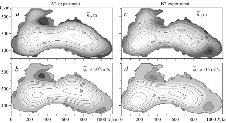
In B2 and A2 experiments in order to relieve barotropic component of currents was set (rb = 0.1 cm/s) more by an order of the bottom friction. As a result, in A2

experiment (Fig 6, a – e) under the constant Coriolis parameter the large-scale circulation separation into individual cyclonic eddies, as in A1 Experiment, did not take place. There was a large cyclonic gyre observed in the sea. It occupied the central part of the basin. On its periphery mesoscale anticyclones periodically arose. They moved along the coast in the direction of the main stream. The areas of anticyclonic vorticity (hydrodynamic instability of currents) were mainly tied to the protruding features of the coastline.

Taking into consideration β-effect in В2 experiment (Fig. 6, f – j), in

comparison with А2 one, the separate eddy formations began to be more clearly

identified in the instantaneous fields, especially in ψ and u2 fields (Fig. 6, i, j).

Although in general circulation changed little.

In the mean fields ψ and h1 in В2 experiment (Fig. 7) the west intensification

of currents is visible and the area of anticyclonic vorticity at the eastern boundary of the basin appeared. In addition, in the averaged field h1 the cyclonic circulation

in the basin center has two centers ("Knipovich glasses"), which was not observed

Fig. 6. Instantaneous distributions of the characteristics in А2 (left) and В2 (right) experiments

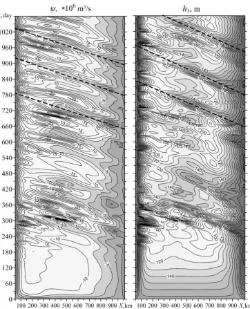
Like in B1 experiment, the eddy formations represented in the instantaneous

fields moved in the western direction. It is well observed on the time diagrams ψ and h1, built for the section Y = 270 km (Fig. 8). In diagram ψ the waves moving

from the east to the west with the phase velocity of 7 – 8 cm/s are clearly

identified. In the field h1 (Fig. 8, b) the phase velocity of the observed waves is less

Fig. 7. Mean distributions h1 and ψ in А2 (left) and В2 (right) experiments

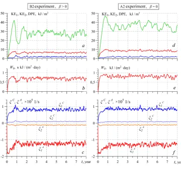
Fig. 9 shows graphs of KE1, KE2, DPE, Wτ, ξ₁C, ξ₂C ξ₁Aand ξ₂A, plotted for

А2 and В2 experiments. It is clear that as compared with А1 and В1 experiments (Fig. 5, а, d)the more intense bottom friction leads to a significant decrease of KE2

and increase of DPE, with practically unchanged KE1.

β-effect in В2 experiment (Fig. 9, а) caused the energy decrease (especially

DPE) comparing with А2 experiment (Fig. 9, d), at that the vorticity features (Fig. 9, c, f) did not changed significantly.

Summarizing the results of B1 and B2 experiments, we can assume that in the Black Sea under the cyclonic wind influence the role of β-effect leads to the formation of long-period waves, which are manifested in the form of alternating eddies moving in the western direction. These waves can be most clearly traced in the field ψ.

Similar results have already been obtained and are described in the papers [7 – 9]. In [8] to determine the nature of the observed processes, the authors compared the model results with the normal modes of own vibrations of a rectangular basin with a homogeneous liquid, with the length, width and depth roughly corresponding to the Black Sea parameters.

The solution of the system of equations of natural vibrations in β-plane for the rectangular two-layer ocean geostrophic approximation is given in [10]. In this case the system of equations has the following form

(

)

(

)

, 0

1 2 2 2 2

2 1 1 1 1

= − ∂

∂ − ∂ ∂ + ∆ ∂

∂

= − ∂

∂ − ∂ ∂ + ∆ ∂

∂

γψ ψ ψ

β ψ

ψ ψ ψ

β ψ

t E x t

t E x

t ₍₂₎

where ψ1, ψ2 are stream functions, for vertically averaged velocities in the upper

Fig. 8. Time diagramsψ (left) and h1 (right) on the section Y = 270 mm in В2 experiment

Fig. 9. Graphs of the KE1, KE2 and DPE energy in В2 – а and А2 – d experiments; tangential wind

stress work Wτ in В2 – b and А2 – e experiments; mean vorticity in В2 – c and А2 – f experiments

Multiplying the second equation of the system (2) by an arbitrary constant α, and adding it to the first one, we obtain the following

(

)

(

)

[

(

)

(

)

]

∂ − +

∂ ∂ + + ∆ ∂

∂ _{ψ αψ β ψ αψ ψ αα γ ψ αα}

t E x

t , (3)

where α₀=h₁ h₂.

Then we are to define a new dependent variable F and an arbitrary constant G:

(

)

(

)

[

]

F =ψ₁+αψ₂ =ψ₁1−αα₀γ +ψ₂ αα₀−1 , (4)

as a result we obtain the following equation of the normal vibrations

0

1 =

∂ ∂ − ∂ ∂ + ∆ ∂

∂

t F G E x F F

t β . (5)

γ αα0 1 1 − = G , γ αα αα α 0 0 1 1 − −

= . (6)

To determine α we obtain a quadratic equation as follows

0 1 2 1 0 0 0

2₊ − _{− =}

γ α α γ α α α ,

from which we find

(

)

α =− −  − + . (7)

Taking into account Fi =ψ1+αiψ2 (i = 1, 2) the equation (5) is rewritten in

the following way:

0 1 = ∂ ∂ +       − ∆ ∂ ∂ x F F G E t i i i

β . (8)

The expression (8) is a well-known equation of planetary waves [15]. It defines two normal fluctuations (barotropic and baroclinic modes) with frequencies σi in a

rectangular basin with the a × b dimensions at Fi = 0 on the boundary expressed by the formula below

2 1 1 2 2 2 2 2 2 2 / −       + + = i i G E b n a

mπ π

β

σ , (9)

where i = 1, 2; m and n are whole numbers.

Taking into account (6) and (7), two values for E₁ G_ican be found:

) ( _{1 2}

2 1 1 h h g f G E + = , 2 1 2 1 2 2 1 h h g h h f G E ε ) ( + = .

The first expression defines a value for the barotropic oscillation mode with an equivalent depth of H = h1 + h2, the second one – for the baroclinic modes with

equivalent depth of

)

( 1 2

2 1 h h h h H + =ε .

Solution of the equation (8) for a rectangular basin with the a × b dimensions under Fi= 0 on a solid boundary was first obtained by Longuet-Higgins [15] and

has the following form

(

)

y b n x a m

Fi γi σi

π π ₊            

=sin sin cos , (i = 1, 2), (10)

where x and y are coordinates; m and n are whole numbers;

i i _σ β γ 2 = .

obtained, under i = 2 – the baroclinic one. The phase velocity of the

waveсi =−σiγi−1, the distance between the moving nodes (half

wavelength) 1

2 −

= πσ β

λ_{i i} and the wave period Ti = 2π/ci.

For the rectangular basin with the dimensions of 1125 × 285 km and the depth

H = 2200 m, with two water layers having the parameters, analogical to the experiments considered, for the principal (m = 1, n =1) barotropic normal mode we obtain: c1 = –7.7 cm/s, λ1 = 276 km, T1 = 82.8 days, for the principal baroclinic

mode: c1 = –0.5 cm/s, λ1 = 69 km, T1 = 331 days. The wave, related to the main

barotropic normal mode has maximum phase velocity. Baroclinic normal modes under the same values of m and n are have smaller phase velocities and wavelengths, than the barotropic modes.

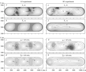
In B1 and B2 experiments, phase velocities of the observed waves (Fig. 4, 8) were obtained close enough to the above calculated velocity of the main barotropic modes of natural oscillations in a rectangular basin. But such a comparison may not look correct due to the strong differences in the shapes of the compared basins. In addition, the calculations using the same formula (10) with different sizes of a rectangular basin showed that the basin width b (the size according to the Y-axis) has the greatest effect on the results, and in case of a real configuration it is very difficult to determine the equivalent width of the sea. Therefore additional B3 experiment was carried out in an elongated basin with constant width and boundaries rounded off to the east and west (Fig. 10). As shown in [2], this form allows you to minimize the nonlinearity effect associated with the basin asymmetry and the coastline roughness. The length, width and depth matched the dimensions of the rectangular basin, the normal modes were calculated for. In addition, to compare and control A3 experiment was carried out, which differs from B3 one by zero value of β-parameter.

Instantaneous distributions h1 and ψ, obtained after the problem entrance in the

statistical equilibrium mode in B3 and A3 experiments and giving an idea of the circulation in the upper and lower layer, are shown in Fig. 10, a, b, d and e. Distributions of the other characteristics are not presented, as there is a good

cross-correlation between fields h1, ζ, u1 and ψ, u2, as well as in the previously considered

pairs of the experiments. As it can be seen in Fig. 10, а – d, in A3 experiment the large-scale circulation was divided into three rounded shape cyclones with a diameter equal to the basin width. Two zones are located between the cyclones. There are mesoscale anticyclonic eddies periodically encountered (Fig. 10 a, b). In the averaged field h1 (Fig. 10, c, d) cyclonic circulations are only observed. Some

anticyclonic eddies are not expressed because of their unsteadiness. In ψ field (Fig. 10, d) two anticyclonic vorticity areas are observed between the three stationary cyclones.

in the instantaneous fields, are not manifested. A slight thickening of the contour as a result of the intensification of western currents is observed near the western coast.

Fig. 10. Instantaneous and mean fieldsin А3 experiment: h1 – a; h1 – b; ψ – c; ψ – d, Instantaneous

and mean fieldsin B3 experiment: h1 – e; h1 – f; ψ – g; ψ – h

In B3 experiment all the eddy formations move in the western direction. This is clearly shown in Fig. 11 (left). There the successive fields ψ, built in the period of 15 days, are demonstrated. If they are compared with the main barotropic normal mode distribution, calculated with the same frequency (Fig. 11, right), great similarity will be found. Also, time diagrams ψ and h1, built for the latitudinal

section passing through the central axis of the basin (Fig. 12), are in a very good agreement with the barotropic normal mode. All the diagrams clearly show wave with a period of 90 days, moving in the western direction with the phase velocity of 7.5 cm/s. Thus, it is possible to make presumptive conclusion that by accounting for the influence of β-effect in B1, B2 and B3 numerical experiments the Rossby waves were obtained. They correspond to the normal barotropic modes of natural oscillations in a closed basin. These waves can be best seen in the field ψ, which characterizes the barotropic component of currents. In diagram h1 (Fig. 12, c) you

Rossby wave background in the areas of positive values of ψ, which correspond to anticyclones.

Fig. 12. Consistent spatial distributions at the latitudinal sections along the central axis of the basin for ψ, corresponding to the normal mode (left) in B3 experiment (center), h1 in B3 experiment (right)

As for the Rossby waves caused by baroclinic modes of the normal vibrations, which, according to theory, should also be present in the solution, they were failed to be identify explicitly in the considered experiments. Most likely, this is due to the fact that the self-oscillating process, changing the sink of energy from the wind and resulting in the oscillation of the observed waves, has the frequency the barotropic Rossby waves predominantly occur at. Theoretical ocean response research on the different types of external exposure is considered in [14]. It is shown that the external effect at the intervals of several weeks – months mostly results in the barotropic Rossby waves. But for the baroclinic waves to appear the oscillating force frequency should be more than a year.

Analysis of the behavior of energy characteristics showed that the β-effect reduces the tangential wind stress work, which in its turn determines the lower level of the energy components calculated in the model. Rossby waves have a stimulating effect on the processes of hydrodynamic instabilities that lead to the appearance of opposite wind vorticity mesoscale eddies.

On the basis of the performed experiments we can agree with the conclusion of the authors of the article [8] that the β-effect and associated Rossby waves in the Black Sea can have a significant impact on the formation of large-scale circulation, comparable to the baroclinic instability effect.

REFERENCES

1. Pavlushin, A.A., Shapiro, N.B., Mikhaylova, E.N. & Korotaev, G.K., 2015, “Two-layer eddy-resolving model of wind currents in the Black Sea”, Physical oceanography, no. 5, pp. 3-12. 2. Pavlushin, A.A., Shapiro, N.B., Mikhaylova, E.N, 2016, “Effect of the basin shape on

formation of the Black Sea circulation”, Physical oceanography, no. 2, pp. 3-15.

3. Seidov, D.G., 1989, “Sinergetika okeanskikh protsessov [Synergetics of the ocean processes]”, Leningrad, Gidrometeoizdat, 288 p. (in Russian).

4. Gill, A., 1986, “Dinamika atmosfery i okeana. T. 1 [Atmosphere and ocean dynamics. Vol. 1]”, Moscow, Mir, 396 p. (in Russian).

5. Kamenkovich, V.M., Monin, A.S., 1978, “Fizika okeana. T. 2-Gidrodinamika okeana [Ocean physics. T2-Ocean hydrodynamics]”, Moscow, Nauka, 435 p. (in Russian).

6. Kamenkovich, V.M, Koshlyakov, M.N. & Monin, A.S., 1987, “Sinopticheskie vikhri v okeane

[Synoptical eddies in the ocean]”, Leningrad, Gidrometeoizdat, 510 p. (in Russian).

7. Rachev, N.H., Stanev, E.V., 1997, “Eddy processes in semi-enclosed seas: A case study for the Black Sea”, J. Phys. Oceanogr., no. 27, pp. 1581-1601.

8. Stanev, E.V., Rachev, N.H., 1999, “Numerical study on the planetary Rossby waves in the Black Sea”, J. Mar. Sys., no. 21, pp. 283-306.

9. Demyshev, S.G., Korotaev, G.K. & Kuftarkov, A.Yu., 1996, “Analiz nachal'nogo perioda prisposobleniya geofizicheskikh poley Chernogo morya k novoy chislennoy modeli [Analysis of the initial adaptation period of the Black Sea geophysical fields to the new numerical model]”, Izv. RAN. FAO, vol. 32, no. 5, pp. 635-644 (in Russian).

10. Korotaev, G.K., Saenko, O.A. & Koblinsky, C.J., 2001, “Satellite altimetry observation of the Black Sea level”, J. Geophys. Res., iss. 106, no. C1, pp. 911-933.

11. Blatov, A.S., Bulgakov, N.P. & Ivanov, V.F. [et al.], 1984, “Izmenchivost' gidrofizicheskikh poley Chernogo morya [Variability of hydrophysical fields of the Black Sea]”, Leningrad, Gidrometeoizdat, 239 p. (in Russian).

12. Latun, V.S., 1989, “Antitsiklonicheskie vikhri v Chernom more letom 1984 goda”, Morskoy gidrofizicheskiy zhurnal, no. 3, pp. 27-34 (in Russian).

13. Latun, V.S., 1990, “Energosnabzhenie glubokikh antitsiklonicheskikh vikhrey Chernogo morya [Power supply of the Black Sea deep anticyclonic eddies. Complex oceanographic research of the Black Sea: Proceedings]”, Kompleksnye okeanograficheskie issledovaniya Chernogo morya: Sb. nauch. tr., pp. 10-21 (in Russian).

14. Safronov, G.F., 1985, “Vozbuzhdenie dlinnykh voln v okeane krupnomasshtabnymi izmeneniyami v pole kasatel'nogo napryazheniya vetra [Oscillation of long waves in the ocean by large-scale changes in the tangential wind stress]”, Moscow, Gidrometeoizdat, 108 p. (in Russian).