https://doi.org/10.5194/ars-15-283-2017
© Author(s) 2017. This work is distributed under the Creative Commons Attribution 3.0 License.
Comparison of digital beamforming algorithms for 3-D terahertz
imaging with sparse multistatic line arrays
Bessem Baccouche1, Patrick Agostini1, Falco Schneider1, Wolfgang Sauer-Greff2, Ralph Urbansky2, and Fabian Friederich1,3
1Fraunhofer Institute for Industrial Mathematics, 67663 Kaiserslautern, Germany
2Institute of Communications Engineering, Kaiserslautern University of Technology, 67663 Kaiserslautern, Germany 3Department of Physics and Research Center OPTIMAS, University of Kaiserslautern, Germany
Correspondence:Fabian Friederich ([email protected])
Received: 9 January 2017 – Revised: 8 August 2017 – Accepted: 14 September 2017 – Published: 12 December 2017
Abstract. In this contribution we compare the back-projection algorithm with our recently developed modified range migration algorithm for 3-D terahertz imaging using sparse multistatic line arrays. A 2-D planar sampling scheme is generated using the array’s aperture in combination with an orthogonal synthetic aperture obtained through linear move-ment of the object under test. A stepped frequency contin-uous wave signal modulation is used for range focusing. Comparisons of the focusing quality show that results us-ing the modified range migration algorithm reflect these of the back-projection algorithm except for some degradation along the array’s axis due to the operation in the array’s near-field. Nevertheless the highest computational efficiency is obtained from the modified range migration algorithm, which is better than the numerically optimized version of the back-projection algorithm. Measurements have been per-formed by using an imaging system operating in theW fre-quency band to verify the theoretical results.
1 Introduction
The use of the effective aperture of a sparse multistatic ar-ray reduces the number of required transmitters (Tx) and receivers (Rx) and preservers the array’s imaging quality
(Lockwood et al., 1996). Hence, this approach is widely spread in the fields of radar and ultrasonic imaging (Wies-beck and Sit, 2014; Thomenius, 1996). The principle idea of the effective aperture concept is to illuminate the target ob-ject with an array of transmitters (Tx-array) and record
back-scattered radiation using an array of receivers (Rx-array).
The Tx-array and the Rx-array are designed in a way that
the convolution of their apertures results in a dense effective aperture. In a subsequent step digital beam forming (DBF) algorithms are applied to the recorded data for 3-D image reconstruction of the target object. Furthermore, the use of DBF techniques does not pose any constraints on the kind of aperture sampling. So one can replace a physical array by an equivalent synthetic one, or combine both or even generate a sampling aperture that corresponds to the object shape. This approach has been adopted in different system designs. In Zhuge and Yarovoy (2011) for instance, the authors reported on the development of an imaging system at a center fre-quency of ca. 11 GHz, which generates a 2-D sampling aper-ture through combining a sparse multistatic line array with a synthetic aperture generated by the movement of the array. However, in Ahmed et al. (2011) the authors used a 2-D pla-nar array for 3-D imaging at a center frequency of 76 GHz. In the field of terahertz imaging there is also a growing inter-est for using sparse arrays, since imaging using quasi-optics in combination with scanning stages doesn’t fulfill real-time operation requirements and focal-plane arrays (FPAs) pose a trade-off between the system’s field of view and the resolu-tion (Friederich et al., 2011). Hence, a major concern about such systems is the acceleration of data acquisition processes as well as faster image generation.
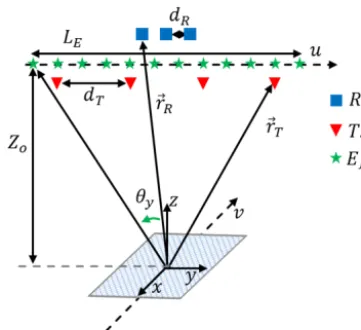
Figure 1.Schematic of a generic imaging setup using the effective aperture concept in combination with a synthetic aperture.
and bistatic configurations (Soumekh, 1991; Lopez-Sanchez and Fortuny-Guasch, 2000). Under the assumption of a fully populated multistatic array an implementation of the RMA is presented in Zhuge and Yarovoy (2011). However, the use of sparse arrays hinders a direct implementation of the RMA because of the violation of the Nyquist sampling criterion along the sampling aperture.
In this contribution we compare a modified RMA with the projection (BP) algorithm and the fast-factorized back-projection (FFBP) algorithm by taking the focusing quality and the asymptotic computing complexity as criteria.
This paper is organized as follows. In Sect. 2 we formulate the imaging problem. The imaging algorithms are briefly de-scribed in Sect. 3. Required sampling criteria and resulting resolution are discussed in Sect. 4. The algorithms are com-pared in Sect. 5. In Sect. 6 terahertz image reconstructions using the mentioned algorithms from measurement data are presented. Conclusions are drawn in Sect. 7.
2 Formulation of the imaging problem
A schematic of the exemplary imaging scenario is depicted in Fig. 1. Along theyaxis a line array ofNTtransmitters il-luminates the measurement scene. The transmitters are oper-ated sequentially. A line array ofNRreceivers records back-scattered radiation from the scene. The Tx-array and Rx -array are placed on the same distanceZofrom the center of the volume to be imaged (for the sake of clarity they are il-lustrated separately). The coordinates of the transmitters and receivers are then given byrT=(0, uT,Zo)andrR=(0, uR,
Zo), respectively. The elements of each array are uniformly
distributed along theyaxis. Both arrays are combined to gen-erate an equivalent effective aperture. Under far-field condi-tions the resulting effective aperture is the convolution of the apertures of theTx-array and theRx-array (Lockwood et al.,
1996). Hence the resulting number of effective sampling
ele-ments isNE=NT×NR. The main idea of this approach is to design the aperture of one array, here theTx-array, in a sparse fashion of the required effective aperture and to design the other array, here respectively theRx-array, in a denser
fash-ion so that its aperture is used as an interpolatfash-ion functfash-ion. Thus, the element spacing in the effective aperture is equal to theRx-array element spacingdR. To generate a uniform ef-fective aperture, the element spacing in theTx-array should
bedT=NR×dR. The coordinates of an effective aperture element are given by,
xE=0,
yE=uT+uR=u,
zE=Zo. (1)
The overall extent of the effective aperture is given byLE=
(NE−1)×dR. The target object is translated along thexaxis, thus mechanically creating a synthetic aperture orthogonally to the array’s aperture. The translation along thex axis is described by the vectorrv=(v,0,0). The signal measured at the effective aperture positionuand the synthetic aperture positionvis given by,
S(u, v, k)= Z
V
o(r)e−j krmu(v,uT,uR,r)dV . (2)
Whereo(r)is the object reflectivity function,V is the illu-minated volume andk=ω/cis the wavenumber composed of the temporal radial frequency ω and the vacuum speed of lightc. Amplitude variations due to antenna patterns and wave propagation attenuation of the volume elements (vox-els) specifying the object are included ino(r).rmuis the path of the electromagnetic waves travelling from an arbitraryTx
to a an arbitrary voxel located atr=(x, y, z)and back to an arbitraryRx,
rmu(v, uT, uR,r)= q
(v−x)2+(u
T−y)2+(Zo−z)2
+ q
(v−x)2+(u
R−y)2+(Zo−z)2. (3) The aspect angle between a voxel and an effective aperture element is denoted byθy. Through combining the effective
aperture of the physical multistatic line array and the syn-thetic aperture generated by the movement of the object we generate a 2-D sampling aperture containingNE×NS sam-pling positions with NS the number of the synthetic aper-ture sampling positions. The requiredNS is estimated using the spectral support along the synthetic aperture as shown in Sect. 4. Range focusing is obtained using a stepped fre-quency continuous wave (SFCW) modulation withNF fquency points. The goal of an imaging algorithm is to re-trieve the object functiono(r). A common method to solve this problem is to use a spatial variant Matched-Filter (Pas-torino, 2010),
o(r)=X
u X
v X
k
where now u comprises all NE measurement positions, v allNS synthetic aperture positions andkallNF SFCW fre-quency points. The reconstruction of 3-D images using a di-rect implementation of Eq. (4) has a high computational load, which makes it unsuitable for time critical imaging appli-cations. By settingM=NE=NS=NF, the reconstruction of N3 voxels using a direct implementation of Eq. (4) has a computational burden of O(N3M3). The computational costs of the implementation of Eq. (4) can be reduced using the following algorithms.
3 Imaging algorithms 3.1 The BP algorithm
Assuming that the measured signal stems from a set of point sources distributed within a volume to be inspected, this al-gorithm projects the measurement data back to their sources. Details on the algorithm can be found in Ulander et al. (2003). Here only the main implementation steps are men-tioned. Starting from a SFCW signal the first step is to inverse Fourier transform the measurement data along the frequency axis
S(u, v, ρ)=Fk−1{S(u, v, k)}. (5) Where ρ is the range variable and numerically performed using the FFT. In this way the data are range focused. The image is reconstructed by estimating the reflectivity of each voxel through linear interpolating the range focused data ac-cording to its relative coordinates to the sampling aperture,
eo(r)= X
u X
v
S(u, v, ρ= |r−a|) , (6)
witha=(v, u, Zo)atNEpositionsuandNSpositionsv. 3.2 The FFBP algorithm
This is a numerically optimized implementation of the BP algorithm. The optimization is based on reducing the com-putational costs of the summation in Eq. (6). Through itera-tively dividing the total volume in sub-volumes and assigning samples from adjacent aperture positions to the centers of the sub-volumes the total number of summations in Eq. (6) is re-duced. The performance of this algorithm is governed by a so called factorization factorn, which denotes the number of adjacent aperture positions taken to form a single new aper-ture position. A more detailed description can be found in Ulander et al. (2003).
3.3 The modified RMA
From Eq. (4) we see thato(r)is estimated through 3-D con-volution in the aperture coordinates (uT, uR, v), which can be implemented in the wavenumber-domain using a complex
multiplication. This is the basic idea of the RMA. However the thinning of theTx-array violates the Nyquist sampling criterion along the axis of theTx-array and leads to alias-ing in the wavenumber-domain. This can be modified to be suitable for imaging with sparse arrays. In the following the main steps of the modified RMA are summarized. Since in the array’s near-field the effective aperture approach is ap-proximately valid due the spherical phase front, a phase com-pensation factor is obtained by calculating the difference be-tween the measured phase and the intended far-field phase in the volume center. Then the measured signal is Fourier trans-formed along the sampling aperture,
S(kx, ky, k)=F(u,v){S(u, v, k)}. (7)
The next step is a regridding of S(kx, ky, k) known as the Stolt interpolation (Cafforio et al., 1991),
S(kx, ky, k)→S(kx, ky, kz) (8)
with
kz= r
k+
q k2−k2
y 2
−k2
x. (9)
This can be obtained by evaluating the Fourier transform in Eq. (7) using the method of stationary phase, which is dis-cussed in more detail in Appendix A. A first estimate of the reflectivity function is obtained by inverse Fourier transform-ing the 3-D spectrum with respect tokxandky,
eo1(r)=F −1
kx,ky{S(kx, ky, kz)}. (10)
The last step is to correct the range curvature in the first esti-mation due to near-field operation,
eo(r)=F −1
kz n
eo1(x, y, kz)e −jkz2
√
x2+y2+Z2
o o
. (11)
4 Sampling constraints and resolution
For a correct reconstruction of the object sampling straints in the space domain have to be fulfilled. These con-straints and the expected spatial resolution are discussed in the following paragraphs. For an extended discussion we re-fer to Soumekh (1994).
4.1 Spatial sampling with a physical aperture
The spacingdRis determined with the knowledge of the spa-tial frequency (wavenumber) supportyof the recorded sig-nal with respect toy,
dR≤ 2π
2y
= π
(ky,max−ky,min)
. (12)
Whereky,maxandky,minare the extrema of theycomponent
kyof the wavenumberkand are given by,
ky,min=ksin(θy,min). (14) For a symmetric imaging setupky,max= −ky,min,
dR≤
π
2ksin(θy,max)
. (15)
The expected spatial resolution along the y axis is also a function of the spatial frequency supporty. The bandwidth
of the spatial spectral support depends on the relative posi-tion of a voxel to the array. For the center of the object the spatial resolution is given by
δy=
2π
y (16)
=
π q
L2E+4Z2
o
kLE
.
4.2 Spatial sampling with a synthetic aperture
Along the x axis the translation movement is used to gen-erate a synthetic aperture in this direction. Sampling con-straints are also derived from the spatial frequencyxof the recorded signal with respect tox. The maximum step size is then given by
dv≤ 2π 2x
= π 4ksin(θ3 dB/2)
. (17)
Where the half-power beamwidth of aTx/Rxantenna is
de-noted by θ3 dB. Using a synthetic aperture we can ensure a constant spatial spectral bandwidth for all parts of the object. The expected spatial resolution in this direction is given by
δx= π
2ksin(θ3 dB/2)
. (18)
4.3 Frequency sampling and range resolution
The range resolution is determined by the signal modulation bandwidthB. For free space wave propagation it is given by
δr≤
c
2B. (19)
Since we use a SFCW waveform, a maximum temporal fre-quency step size1fis required in order to avoid range ambi-guities. For a required range unambiguityRun,
1f≤
c
2Run
. (20)
5 Comparison of the algorithms 5.1 Focusing quality
Firstly, we compare the focusing quality of the BP algorithm, FFBP algorithm and the RMA using numerical simulations.
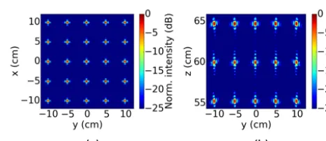
Figure 2.3-D image reconstruction using the BP algorithm.(a)xy -section atz=Zo.(b)yz-section atx=0.
Figure 3. 3-D image reconstruction using the FFBP algorithm. (a)xy-section atz=Zo.(b)yz-section atx=0.
Assuming that the required spatial resolution is 4 mm, ac-cording to Eqs. (12) and (16), an effective aperture of 50 cm is required at an imaging range ofZo=60 cm. The spacing between the receiver elements has to be at most 2 mm in or-der to avoid aliasing. Hence we assume aRx-array with 10 elements spaced by 2 mm and aTx-array containing 25 Tx
with an element spacing of 2 cm to obtain the required ef-fective aperture. The corresponding number of efef-fective ele-ments is 250 eleele-ments. We also assume a synthetic aperture of 25 cm. According to Eq. (17) the sampling step along the synthetic aperture has to be at most 1 mm. We use an SFCW waveform with 300 frequency steps from 75 to 110 GHz. We simulate the signal from a 3-D grid of ideal point reflectors with a uniform spacing of 5 cm using Eq. (2) and reconstruct it using the proposed RMA, the BP algorithm and the FFBP algorithm.
The implementation of the two latter algorithms requires the definition of a discrete 3-D rectangular volume, which covers the expected extent of the target. The distances be-tween each two points of the volume is set to half of the ex-pected resolution along each dimension. Two perpendicular sections from the image reconstruction obtained using the BP algorithm are depicted in Fig. 2. Figure 2a shows anxy -section of the volume, which describes the estimated object reflectivity at a constant depthz=Zo. This section shows a
-Figure 4.3-D image reconstruction using the modified RMA algo-rithm.(a)xy-section atz=Zo.(b)yz-section atx=0.
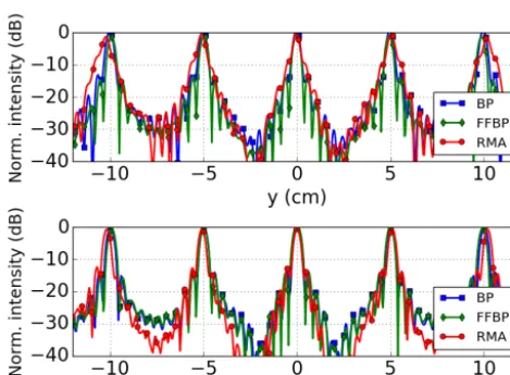
Figure 5.Focusing quality comparison of the modified RMA with the BP and FFBP algorithms.
section and yz-section, which result from the FFBP algo-rithm with a factorization factor ofn=2 are shown in Fig. 3a and b, respectively. They also demonstrate the successful 3-D focusing using this algorithm. Finally the same sections, which result from the proposed RMA are provided in Fig. 4 to illustrate its 3-D focusing quality.
For a quantitative assessment of the imaging quality, we take a closer look at the focusing along theyaxis andxaxis of each algorithm. The upper part of Fig. 5 shows three
y profiles of the estimated reflectivity function atx=0 and
z=Zo. The profiles resulting from the BP and FFBP agree very well. The 3 dB-width of the main lobes yield a width of ca. 4 mm. The side lobes level is ca.−14 dB due to the rect-angular shape of the aperture. The width of the main lobes of the profile resulting from the RMA fulfill the expected resolution, yet with increasing y-coordinate the RMA main lobes yield a slight shift accompanied by a broadening. An increase of the side lobes level of the RMA by ca. 3 dB is also observable. Thex-profiles of the algorithms aty=0 and
z=Zoare depicted in the lower part of Fig. 5. Along with
the x axis the 3 dB-width of the main lobe of the three al-gorithms agree very well. All alal-gorithms achieve the desired resolution of 4 mm. Along this axis the RMA yield solely a
Figure 6.Reconstruction time comparison of the modified RMA with the BP and FFBP algorithms.
slight shift with increasingxcoordinate. The behavior of the RMA is expected, due to the approximately validness of the effective aperture approach in the near-field of the array. It is worth mentioning, that although the synthetic aperture is as large as half of the effective aperture, both achieve the same spatial resolution. This is due to the spectral support of the synthetic aperture, which is two times higher than the one of the effective aperture, compare Eqs. (16) and (18).
5.2 Computational complexity
Secondly, we compare the computing costs of the three dis-cussed algorithms. Using the asymptotic computational com-plexity of the implementation steps of each algorithm we can estimate its computational burden. For the RMA the highest computational burden is caused by the 3-D Stolt interpola-tion. Since this is implemented using a complex 3-D linear interpolation, its asymptotic operation countCpis
Cp=O(M3). (21)
Additionally we use in this algorithm 5 complex FFT opera-tions with a total asymptotic operation countCfftof,
Cfft=O 5M
2 log2(M)
. (22)
Hence the asymptotic computing complexity of the RMA is,
CRMA=O(Cfft+Cp)
=O 5
M
2 log2(M)+M 3
. (23)
The computational burden of the BP algorithm is estimated from Eqs. (5) and (6),
CBP=O
N3M2+M
2 log2(M)
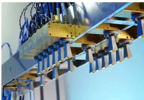
Figure 7.Multistatic sparse line array composed of 12Tx and 12
Rx.
For an aperture factorization factornthe computational load of the FFBP algorithm is given as function of the computa-tional load of the BP algorithm (Ulander et al., 2003),
CFFBP=O nlog
n(M)
M CBP
=O
nlogn(M)
N3M+1
2log2(M)
. (25)
For large volumesN3M1
2log2(M)
,
CFFBP≈O
nlogn(M)N3M. (26)
Comparing the FFBP with the RMA we obtain a computa-tional saving in the order of
CFFBP
CRMA
=O nlogn(M)N 3M 5M
2 log2(M)+M3 !
=O nlogn(M)N 3 5
2log2(M)+M2 !
. (27)
By setting N=M we obtain the computational saving as function of amount of measurement samples,
CFFBP
CRMA
=O nlogn(M)M. (28) Furthermore, we have compared the performance of the men-tioned algorithms on a commercial i7 CPU with 3.5 GHz and 16 GB of RAM. The scientificPythonmodules (van der Walt et al., 2011) have been used for the implementation of the algorithms. Using numerical simulation we investigate the dependency of the reconstruction time on the amount of vox-els to be reconstructed for each algorithm. The results are depicted in Fig. 6. The x axis of Fig. 6 represents the total
Figure 8. A-sandwich GFRP with a Rohacell core with a size of (20 cm×10 cm× 0.5 cm): (a) Photograph of the sample. (b)Schematic and distribution of defects.
number of the image voxels (N3). As expected the highest reconstruction duration is caused by the BP algorithm. This increases rapidly with increasing number of voxels. A sig-nificant improvement is obtained using the FFBP algorithm. For instance, the reconstruction of 100 Kilovoxels becomes four times faster. However, the modified RMA yields the best computational performance. The 100 Kilovoxels have been reconstructed 22 times faster than the FFBP algorithm and 90 times faster than the BP algorithm. Significantly faster recon-struction times can be obtained by parallelizing the imple-mentation of the algorithms as reported in Baccouche et al. (2017), where the mentioned algorithms are executed on a graphics processing unit.
6 Measurement results
We experimentally investigated the imaging performance of the algorithms using measurement data from the imaging system presented in Baccouche et al. (2015), which combines a sparse line array with a band-conveyor for 3-D tera-hertz imaging as sketched in Fig. 1. This system operates in the
W-band and provides a modulation bandwidth of 35 GHz. As Fig. 7 shows, the multistatic sparse line arrays used in this system contains 12 transmitters, which are linearly dis-tributed along the y axis. Standard-gain horn antennas are used for the transmitters as well as for the receivers. The transmitters are sequentially operated using a switching ma-trix. TheRx-array contains also 12 elements. For the ease of
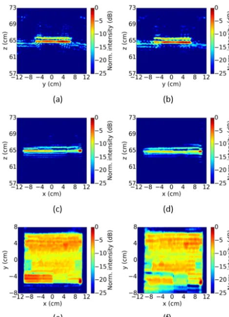
Figure 9. 3-D terahertz image reconstruction of the GFRP sam-ple:(a),(c)and(e)yz-section,xz-section andxy-section using BP, respectively.(b),(d)and(f)yz-section,xz-section andxy-section using modified RMA, respectively.
As measurement sample we used an A-sandwich (20 cm×10 cm×0.5 cm) made of glass fiber reinforced plastic (GFRP) with a Rohacell core, depicted in Fig. 8a. The sample was prepared with different insertions at differ-ent locations with varying depths on the top of the Rohacell core. Figure 8b shows a schematic of the sample with the different insertions and defects, which are made of adhesive, teflon and polyethylene (PE). Furthermore, a step wedge was formed at the top of the sample through removing surface layers. The step size is less than 1 mm. The corner of the sample was marked with an aluminum quadrant. The imag-ing range is ca. 65 cm. Figure 9 shows different 2-D layers from the 3-D image reconstruction of the sample using the BP algorithm as a reference (Fig. 9a, c and e) and the mod-ified RMA (Fig. 9b, d and f). By comparing Fig. 9e and f, the same amount of defects at this layer can be recognized using both algorithms even if the modified RMA yields the expected degradation with respect to the array’s axis (yaxis). Figure 9c and d shows that the modified RMA is also sensi-tive to the tiny thickness variations of the sample as well as the BP algorithm. The upper and the lower layers of the
sam-ple are resolved by both algorithms (Fig. 9a and b). These two figures show also the expected increase of grating lobes along the array’s axis, yet confirming that the modified RMA approximates well the focusing quality of the BP algorithm.
7 Conclusions
We have compared the back-projection algorithm (BP) and its numerical optimized implementation, the fast-factorization back-projection (FFBP) algorithm, with a mod-ified range migration algorithm (RMA) for 3-D terahertz imaging using a sparse multistatic line array in combination with a synthetic aperture. As criteria for comparison we took the focusing quality and the computational complexity. We have shown that the computational costs can be significantly reduced using the FFBP algorithm with competitive imaging quality to the BP algorithm. On the other side the modified RMA yields the highest computational efficiency at the costs of a minor focusing degradation along the array’s axis due to the operation in the array’s near-field. We used an undersam-pled sparse multistatic line array to inspect the inner structure of a glass fibre reinforced plastics (GFRP) sample in the fre-quency range 75 to 110 GHz. Using the modified RMA we can recognize the same relevant features within the sample as by using the BP algorithm with dramatically reduced compu-tational effort.
Appendix A: Fourier transform using the method of stationary phase (MSP)
The relation given in Eq. (9) results from applying the MSP to asymptotically evaluate the 2-D Fourier transform along the measurement aperture,
F (kx, ky)= Z
y Z
x
ej 8(x,y)dxdy , (A1)
with,
8(x, y)=k(r1+r2)−kxx−kyy. (A2)
and
r1= q
x2+y2+(Zo−z)2
r2= p
x2+(Z
o−z)2.
The approximate solution of Eq. (A1) using the MSP is then,
F (kx, ky)≈ej 8(x0,y0). (A3)
Wherex0andy0are the phase stationary points. These can be found by equating the first partial derivatives of8(x, y)
to zero. ∂8(x, y) ∂x
(x0,y0)
=0 (A4)
∂8(x, y) ∂y
(x0,y0)
=0 (A5)
The first partial derivatives of8(x, y)are,
8x(x, y)=
∂8(x, y)
∂x =k
x r1
+x
r2
−kx (A6)
8y(x, y)=
∂8(x, y) ∂y =k
y r1
−ky. (A7)
We solve Eq. (A5) fory0,
kq y0
x2+y2
0+(Zo−z)2
−ky=0 (A8)
y0= ±
ky q
k2−k2
y p
x2+(Z
o−z)2. (A9)
Now we solve Eq. (A4) forx0,
x02
1+ 1
r
1+ y
2 0
x02+(Zo−z)2
2 = kx k 2
x20+(Zo−z)2
.
(A10) By inserting the solution fory0in Eq. (A10) we get,
x02
1+ 1
r 1+ k
2
y k2−k2
y 2 = k x k 2
x02+(Zo−z)2
(A11)
x0= ±
(Zo−z)kx kz
, (A12)
with
kz= r
k+qk2−k2
y 2
−k2
x. (A13)
To obtain the expression ofy0, we insertx0in Eq. (A9),
y0= ±
ky q
k2−k2
y
k+qk2−k2
y
kz
(Zo−z) . (A14)
Since (Zo> z) both first derivatives simultaneously vanish
only for the positive solutions. Now we insert Eqs. (A12) and (A14) in Eq. (A2),
8(x0, y0)=k(Zo−z) v u u u u t
kx2 k2
z
+
k2y
k+qk2−k2
y 2
k2
z
k2−k2
y
+1
+k(Zo−z) s
kx2 k2
z
+1−kx (Z
o−z)kx kz
−ky
ky kz
k+qk2−k2
y
q k2−k2
y
(Zo−z)
. (A15)
After some mathematical rearrangements we obtain,
8(x0, y0)=
k2k+qk2−k2
y
kz q
k2−k2
y
(Zo−z) (A16)
+
kk+qk2−k2
y
kz
(Zo−z)
−k 2
x kz
(Zo−z)
−
k2yk+qk2−k2
y
kz q
k2−k2
y
(Zo−z).
=
k+qk2−k2
y 2 kz −k 2 x kz
=kz(Zo−z) . (A17) By inserting Eq. (A17) in Eq. (A3) we obtain,
Competing interests. The authors declare that they have no conflict of interest.
Acknowledgements. This work was supported by FhG Internal Programs under Grant No. Attract 018-692 158, the FhG pilot project: Fraunhofer innovations for cultural heritage and the Innovation Center of Applied System Modeling for Computational Engineering (ASM4CE) in Kaiserslautern, Germany. The authors would also like to thank Andreas Keil and Georg von Freymann for the fruitful discussions. Finally our thank goes to John D. Hunter for providing the 2-D graphics environment matplotlib (Hunter, 2007).
Edited by: Eckard Bogenfeld
Reviewed by: two anonymous referees
References
Ahmed, S. S., Schiessl, A., and Schmidt, L. P.: A Novel Fully Electronic Active Real-Time Imager Based on a Planar Multi-static Sparse Array, IEEE T. Microw. Theory, 59, 3567–3576, https://doi.org/10.1109/TMTT.2011.2172812, 2011.
Baccouche, B., Keil, A., Kahl, M., Haring Bolivar, P., Loeffler, T., Jonuscheit, J., and Friederich, F.: A sparse array based sub-terahertz imaging system for volume inspection, in: Mi-crowave Conference (EuMC), 2015 European, pp. 438–441, https://doi.org/10.1109/EuMC.2015.7345794, 2015.
Baccouche, B., Agostini, P., Mohammadzadeh, S., Kahl, M., Weisenstein, C., Jonuscheit, J., Keil, A., Löffler, T., Sauer-Greff, W., Urbansky, R., Bolívar, P. H., and Friederich, F.: Three-Dimensional Terahertz Imaging With Sparse Mul-tistatic Line Arrays, IEEE J. Sel. Top. Quant., 23, 1–11, https://doi.org/10.1109/JSTQE.2017.2673552, 2017.
Cafforio, C., Prati, C., and Rocca, F.: SAR data focusing using seis-mic migration techniques, IEEE T. Aero. Elec. Sys., 27, 194– 207, https://doi.org/10.1109/7.78293, 1991.
Friederich, F., von Spiegel, W., Bauer, M., Meng, F., Thomson, M. D., Boppel, S., Lisauskas, A., Hils, B., Krozer, V., Keil, A., Loffler, T., Henneberger, R., Huhn, A. K., Spickermann, G., Boli-var, P. H., and Roskos, H. G.: THz Active Imaging Systems With Real-Time Capabilities, IEEE T. Terahertz Science and Technol-ogy, 1, 183–200, https://doi.org/10.1109/TTHZ.2011.2159559, 2011.
Hunter, J. D.: Matplotlib: A 2D Graphics Environment, Com-put. Sci. Eng., 9, 90–95, https://doi.org/10.1109/MCSE.2007.55, 2007.
Lockwood, G. R., Li, P.-C., O’Donnell, M., and Foster, F. S.: Optimizing the radiation pattern of sparse peri-odic linear arrays, IEEE T. Ultrason. Ferr., 43, 7–14, https://doi.org/10.1109/58.484457, 1996.
Lopez-Sanchez, J. M. and Fortuny-Guasch, J.: 3-D radar imaging using range migration techniques, IEEE T. Antenn. Propag., 48, 728–737, https://doi.org/10.1109/8.855491, 2000.
Pastorino, M.: Microwave Imaging, Wiley, Hoboken, 2010. Soumekh, M.: Bistatic synthetic aperture radar inversion
with application in dynamic object imaging, in: Acous-tics, Speech, and Signal Processing, 1991, ICASSP-91, 1991 International Conference on, 4, 2577–2580, https://doi.org/10.1109/ICASSP.1991.150928, 1991.
Soumekh, M.: Fourier Array Imaging, Fourier Array Imaging, PTR Prentice-Hall, 1994.
Thomenius, K. E.: Evolution of ultrasound beamformers, in: Proceedings of the IEEE Ultrason., 2, 1615–1622, https://doi.org/10.1109/ULTSYM.1996.584398, 1996.
Ulander, L. M. H., Hellsten, H., and Stenstrom, G.: Synthetic-aperture radar processing using fast factorized back-projection, IEEE T. Aero. El. Sys. Mag., 39, 760–776, https://doi.org/10.1109/TAES.2003.1238734, 2003.
van der Walt, S., Colbert, S. C., and Varoquaux, G.: The NumPy Ar-ray: A Structure for Efficient Numerical Computation, Comput. Sci. Eng., 13, 22–30, https://doi.org/10.1109/MCSE.2011.37, 2011.
Wiesbeck, W. and Sit, L.: Radar 2020: The future of radar systems, in: 2014 International Radar Conference, 1–6, https://doi.org/10.1109/RADAR.2014.7060395, 2014.