Geosci. Model Dev., 6, 457–468, 2013 www.geosci-model-dev.net/6/457/2013/ doi:10.5194/gmd-6-457-2013
© Author(s) 2013. CC Attribution 3.0 License.
EGU Journal Logos (RGB)
Advances in
Geosciences
Open Access
Natural Hazards
and Earth System
Sciences
Open AccessAnnales
Geophysicae
Open AccessNonlinear Processes
in Geophysics
Open AccessAtmospheric
Chemistry
and Physics
Open AccessAtmospheric
Chemistry
and Physics
Open Access DiscussionsAtmospheric
Measurement
Techniques
Open AccessAtmospheric
Measurement
Techniques
Open Access DiscussionsBiogeosciences
Open Access Open Access
Biogeosciences
Discussions
Climate
of the Past
Open Access Open Access
Climate
of the Past
Discussions
Earth System
Dynamics
Open Access Open Access
Earth System
Dynamics
DiscussionsGeoscientific
Instrumentation
Methods and
Data Systems
Open Access
Geoscientific
Instrumentation
Methods and
Data Systems
Open Access DiscussionsGeoscientific
Model Development
Open Access Open Access
Geoscientific
Model Development
DiscussionsHydrology and
Earth System
Sciences
Open AccessHydrology and
Earth System
Sciences
Open Access DiscussionsOcean Science
Open Access Open Access
Ocean Science
Discussions
Solid Earth
Open Access Open Access
Solid Earth
DiscussionsThe Cryosphere
Open Access Open Access
The Cryosphere
DiscussionsNatural Hazards
and Earth System
Sciences
Open Access
Discussions
Inclusion of ash and SO
2
emissions from volcanic eruptions in
WRF-Chem: development and some applications
M. Stuefer1, S. R. Freitas2, G. Grell3, P. Webley1, S. Peckham3, S. A. McKeen3, and S. D. Egan1
1Geophysical Institute, University of Alaska Fairbanks, 903 Koyukuk Drive, Fairbanks, Alaska, AK 99775, USA 2Center for Weather Prediction and Climate Studies – CPTEC/INPE, Cachoeira Paulista, 12630-000 Sao Paulo, Brazil 3National Oceanic and Atmospheric Administration Earth Systems Research Laboratory, 325 Broadway, Boulder, Colorado,
CO 80305-3337, USA
Correspondence to: M. Stuefer ([email protected])
Received: 13 July 2012 – Published in Geosci. Model Dev. Discuss.: 3 September 2012 Revised: 27 February 2013 – Accepted: 4 March 2013 – Published: 9 April 2013
Abstract. We describe a new functionality within the
Weather Research and Forecasting (WRF) model with cou-pled Chemistry (WRF-Chem) that allows simulating emis-sion, transport, disperemis-sion, transformation and sedimentation of pollutants released during volcanic activities. Emissions from both an explosive eruption case and a relatively calm degassing situation are considered using the most recent vol-canic emission databases. A preprocessor tool provides emis-sion fields and additional information needed to establish the initial three-dimensional cloud umbrella/vertical distribution within the transport model grid, as well as the timing and du-ration of an eruption. From this source condition, the trans-port, dispersion and sedimentation of the ash cloud can be realistically simulated by WRF-Chem using its own dynam-ics and physical parameterization as well as data assimila-tion. Examples of model applications include a comparison of tephra fall deposits from the 1989 eruption of Mount Re-doubt (Alaska) and the dispersion of ash from the 2010 Ey-jafjallaj¨okull eruption in Iceland. Both model applications show good coincidence between WRF-Chem and observa-tions.
1 Introduction
Past and recent volcanic eruptions, such as Eyjafjallaj¨okull (Gudmundsson et al., 2010) and Puyehue Cordon-Caulle (BVGN, 2011), with huge impacts on the environment (soil, water), air quality and air traffic have been increas-ing the need of accurate real-time forecasts of ash movement
show that online models represent the atmosphere more re-alistically. Errors in air quality prediction introduced by the offline approach can be quite substantial, especially as the model resolution is increased (Grell and Baklanov, 2011). The online approach using the Weather Research and Fore-casting (WRF) with Chemistry (WRF-Chem, Grell et al., 2005) model accounts for a numerically consistent air qual-ity forecast; no interpolation in time or space is required. In this paper we describe how volcanic emissions may be in-cluded in WRF-Chem, and apply the model using emissions from volcanic eruptions. We use WRF-Chem for studies of past volcanic eruptions to better understand volcanic emis-sions and their transport within the atmosphere. Intercom-parison studies of coupled (online) versus decoupled (offline) models will follow based on this work. The modelled feed-back between volcanic emissions is suitable for climate im-pact studies as well as for detailed studies of the dispersion and the weather following an eruption event. In the follow-ing we describe the implementation of generalized volcanic source parameters within WRF-Chem, indicating an oppor-tunity to use the modelling system for near-real-time erup-tions at times during an event when the user might know a location and maybe the height of a volcanic plume, but oth-erwise there is little information available about the charac-teristics of a certain eruption. WRF-Chem is based on the WRF model (Skamarock et al., 2008). The architecture of WRF supports both research and operational weather fore-casting applications. WRF includes various options for dy-namic cores and physical parameterizations (Skamarock et al., 2008) so that it can be used to simulate atmospheric processes over a wide range of spatial and temporal scales. WRF-Chem simulates trace gases and particulates interac-tively with the meteorological fields using several treatments for photochemistry and aerosols developed by the user com-munity. The work described in this paper is based on WRF versions 3.3.1 and 3.4 (WRFV3.4, released in April 2012). A brief description is given at the beginning of Sect. 3.
Section 2 of this paper describes the source parameters that we use to determine volcanic emissions, as well as sulfur dioxide (SO2) from volcanic degassing processes. In Sect. 3
we explain the implementation into WRF-Chem. Section 4 demonstrates two applications. Section 5 discusses some of the software issues. Our conclusions are discussed in Sect. 6.
2 Volcanic emissions
Volcanic ash, SO2, and other trace gases perturb atmospheric
composition and chemistry. Volcanic ash consists of fine-grained rock, mineral fragments, and glass shards gener-ated during eruptions. With any VATD model and especially WRF-Chem, initial source information on the volcanic emis-sions is critical for the model’s ability to forecast the ash cloud movement and provide warnings on actual ashfall con-centrations (Webley and Mastin, 2009). A volcanic plume
model generates the source data for WRF-Chem. The nec-essary parameters are the scale of the eruption including the erupted mass, the initial altitudes of the ash particles and SO2, an eruption rate, and a grain size spectrum of the
ash particles. Mastin et al. (2009) have developed “eruption source parameters (ESP)” for the world’s volcanoes. Each of the world’s volcanoes has a “typical” eruption assigned to it. Mastin et al. (2009) provide details on each source param-eter for each ESP type, which include plume altitude, mass of the eruption cloud and particle size distributions. WRF-Chem uses ESP type data as volcanic emission information for the model forecasting. The modelled volcanic ash is sub-divided into different bins representing the size spectrum of the particles, typically ranging from a few micrometers up to one or two millimeters. We have developed a volcanic emission preprocessor for initializing the ash fields within the model based on a look-up table containing the ESP data. The programming code of the Coupled Aerosol Tracer Transport model, which has been developed for the Brazilian version of the Regional Atmospheric Modelling System (Freitas et al., 2009), has been used as a template and adapted to suit WRF-Chem. In the following subsection we describe how ash and SO2emissions from volcanic activities are formulated for use
in the WRF-Chem model.
2.1 The emissions preprocessor
Table 1. Injection height, duration, eruption rate, volume and mass fraction (<63µm) as provided by Mastin et al. (2009) and used to determine the eruption properties within the WRF-Chem model. Adapted from Mastin et al. (2009).
ESP Type Example Height Duration (h) Eruption Volume Mass
above rate fraction
vent less than
(km) (h) (kg s−1) (km3) 63 micron
M0 standard mafic Cerro Negro, Nicaragua, 4/13/1992 7 60 1×10⁵ 0.01 0.05
M1 small mafic Etna, Italy, 4/13/1992 2 100 5×10³ 0.001 0.02
M2 medium mafic Cerro Negro, Nicaragua, 4/9-13/1992 7 60 1×10⁵ 0.01 0.05
M3 large mafic Fuego, Guatemala, 10/14/1974 10 5 1×10⁶ 0.17 0.1
S0 standard silicic Spurr, USA, 8/18/1992 11 3 4×10⁶ 0.015 0.4
S1 small silicic Ruapehu, New Zealand, 6/17/1996 5 12 2.×105 0.003 0.1
S2 medium silicic Spurr, USA, 8/18/1992 11 3 4×10⁶ 0.015 0.4
S3 large silicic St Helens, USA, 5/18/1980 15 8 1×10⁷ 0.15 0.5
S8 co-ignimbrite silicic St Helens, USA, 5/18/1980 (pre-9 a.m.) 25 0.5 1×10⁸ 0.05 0.5 S9 brief silicic Soufri`ere Hills, Montserrat (composite) 10 0.01 3×10⁶ 0.0003 0.6
U0 default submarine none 0 – – –
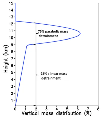
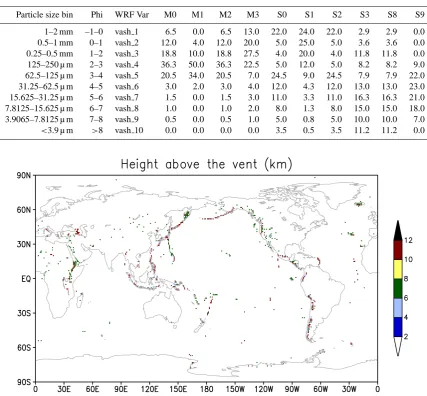
it. The umbrella cloud detrainment layer is represented as a parabolic mass distribution. Note that this method does not account for the detailed dynamics of the erupted plume above the volcano vent; we further do not include any data on the thermodynamics of the eruption itself. Phenomena such as pyrocumuli are not resolved within the model. Data on atmo-spheric heat release during an eruption, or detailed plume dy-namics, are very sparse. The total erupted mass is calculated using the corresponding erupted volume (Table 1) times the ash mass density, which is defined as 2600 kg m−3. Then the total ash mass is distributed between 10 bins of aerosol par-ticles with diameter size range starting from 2 mm down to less than 3.9 µm, using the corresponding percentage of mass derived from analysis of historic eruptions. Table 2 gives the selected particle size bins, which have been associated with the WRF-Chem variable names vash 1 to vash 10, and the corresponding mass fraction percentage for each volcano ESP type. Scollo et al. (2007), Rose et al. (2007), Durant and Rose (2009), Bonadonna and Houghton (2005), Durant et al. (2009), and Bonadonna et al. (2002) used analysis of ash samples mostly from the example eruptions listed in Ta-ble 1 to derive the mass fraction percentage shown in TaTa-ble 2. For each bin the aerodynamic radius, needed by the settling velocity calculation, is defined as half of the arithmetic mean between the limits of the diameters of each bin size. The time interval during which the ash mass is released in the domain of the model simulation is given by the default “duration” parameter as specified in Table 1. If observed data of injec-tion heighthand eruption length d are available, they may be used instead. The 1535 volcanoes with referenced source parameters as specified in Table 1, for which WRF-Chem is able to simulate the associated ash cloud movement in an
Fig. 1. The vertical profile of the ash cloud mass distribution (%) associated with an eruption with 12 km height above the vent. In this case the cloud base is located around 9 km height above the vent. Note the umbrella cloud detrainment layer represented as a parabolic mass distribution with 75 % of the erupted mass. The 25 % of the erupted mass is linearly detrained from the umbrella base to the vent height.
Table 2. Ash particle bin size ranges with corresponding WRF-Chem variable names; the mass fractions in percent of total mass are given below each ESP eruption type M0–M3 and S0–S9.
Particle size bin Phi WRF Var M0 M1 M2 M3 S0 S1 S2 S3 S8 S9
1–2 mm –1–0 vash 1 6.5 0.0 6.5 13.0 22.0 24.0 22.0 2.9 2.9 0.0
0.5–1 mm 0–1 vash 2 12.0 4.0 12.0 20.0 5.0 25.0 5.0 3.6 3.6 0.0
0.25–0.5 mm 1–2 vash 3 18.8 10.0 18.8 27.5 4.0 20.0 4.0 11.8 11.8 0.0 125–250 µ m 2–3 vash 4 36.3 50.0 36.3 22.5 5.0 12.0 5.0 8.2 8.2 9.0 62.5–125 µ m 3–4 vash 5 20.5 34.0 20.5 7.0 24.5 9.0 24.5 7.9 7.9 22.0 31.25–62.5 µ m 4–5 vash 6 3.0 2.0 3.0 4.0 12.0 4.3 12.0 13.0 13.0 23.0 15.625–31.25 µ m 5–6 vash 7 1.5 0.0 1.5 3.0 11.0 3.3 11.0 16.3 16.3 21.0 7.8125–15.625 µ m 6–7 vash 8 1.0 0.0 1.0 2.0 8.0 1.3 8.0 15.0 15.0 18.0 3.9065–7.8125 µ m 7–8 vash 9 0.5 0.0 0.5 1.0 5.0 0.8 5.0 10.0 10.0 7.0 <3.9 µ m >8 vash 10 0.0 0.0 0.0 0.0 3.5 0.5 3.5 11.2 11.2 0.0
Fig. 2. The global dataset of volcanoes described in Mastin et al. (2009) and included in WRF-Chem model to simulate ash cloud movement. The figure shows the plume height above the vent prescribed for each volcano with past and potential future eruption.
2.2 Volcanic SO2degassing emissions
The data provided by the AEROCOM program (http: //www-lscedods.cea.fr/aerocom/AEROCOM\HC/volc/, Diehl, 2009; Diehl et al., 2012) contain volcanic SO2
emissions and other variables for all days from 1 January 1979 to 31 December 2009 for all volcanoes with historic eruptions listed in the Global Volcanism Program database provided by the Smithsonian Institution. There is one file for each year that contains the number of events for each day of that year over the entire world. For each event the volcano name, date, height above the mean sea level, cloud column height, longitude, latitude, and daily emission rate of SO2
are provided. There is also a separation between eruptive and non-eruptive volcanic emissions.
In a similar fashion to the volcanic ash, the emission pro-cessing tool places the SO2emissions from each volcano in
the WRF-Chem grid box, which surrounds its geographical location. The total emission is calculated by summing the emissions of all volcanoes within the grid cell. Next, the to-tal emission and the minimum and maximum column heights of the set of volcanoes within the grid cell are provided. The units are kg [SO2] m−2dy−1. If other observed volcanic SO2
emission data are available (i.e. from satellite retrievals us-ing the Ozone Monitorus-ing Instrument), or SO2emissions are
modelled for volcanic eruptions outside the date range cov-ered by the AEROCOM data, SO2mass emission rates can
be entered in the WRF-Chem emissions driver. In this case the SO2plume resembles the umbrella-shaped plume of the
In general, once airborne, SO2 oxidizes to sulfuric acid
(H2SO4) that condenses into sulfate aerosol, and the
atmo-spheric loading and residence time of the sulfate aerosol is proportional to the sulfur-containing gases in the volcanic plume. As for the ash emissions, to evaluate the impacts of volcanic emissions, it is important to use accurate assump-tions not only of SO2 emission rates, but also of injection
heights. It is important to note that SO2may show different
plume characteristics than volcanic ash; also the residence time of sulfate aerosol may differ significantly from the resi-dence time of ash. An example was the June 1991 eruption of Pinatubo (Philippines), which injected large amounts of SO2
and ash up to 35 km above sea level (a.s.l.) into the strato-sphere. The sulfate aerosol was detected for many months after the eruption, while the ash settled within several days (McCormick et al., 1995).
3 Inclusion of volcanic emissions in WRF-Chem
In this section we describe how ash and SO2emissions from
volcanic activities are used in the WRF-Chem model. WRF’s typical governing equations are fully compressible; the used Advanced Research WRF (ARW) solver includes the non-hydrostatic Euler equations and conserves mass and other scalars (Skamarock et al., 2008). WRF/Chem v3.4 contains two hard coded gas phase chemical mechanisms: the sec-ond generation Regional Acid Deposition Model mechanism (RADM2) (Stockwell et al., 1990), and the Carbon Bond Mechanism version Z (CBM-Z) (Zaveri and Peters, 1999). The kinetic preprocessor (KPP, Salzmann, 2008; Grell et al., 2011b) is also used in WRF-Chem, which allows many ad-ditional gas phase chemical mechanisms. The aerosol mod-ules available in WRFV3.4 are the Modal Aerosol Dynamics Model for Europe (MADE) (Ackermann et al., 1998) with the secondary organic aerosol (SOA) model (SORGAM) of Schell et al. (2001) (referred to as MADE/SORGAM), and the Model for Simulating Aerosol Interactions and Chem-istry (MOSAIC) (Zaveri et al., 2008). The volatility basis set (VBS) approach has been coupled to both MOSAIC (Shrivastava et al., 2011) and MADE (Ahmadov et al., 2012). The numerically very simple and computationally inexpen-sive bulk approach from the Goddard Chemistry Aerosol Ra-diation and Transport (GOCART, Chin et al., 2002) model is also available in WRF-Chem V3.4. An aerosol optical prop-erty module (Fast et al., 2006; Barnard et al., 2010) was added to WRF-Chem that treats bulk, modal, and sectional aerosol size distribution using a similar methodology for re-fractive indices and multiple mixing rules. The WRF-Chem aerosol modules allow for quantification of the interaction between aerosol and precipitation, such as the first aerosol indirect effect (Twomey, 1977) referring to the modification of the cloud droplet number concentration by aerosols, or the second indirect effect, which was first proposed by Al-brecht (1989), who showed that the suppression of
precip-itation by aerosols could increase cloud water content (or cloud liquid water path, LWP) and fractional cloud cover. The interactions between aerosols and clouds, such as the first and second indirect effects, activation/resuspension, wet scavenging, and aqueous chemistry are described in more de-tail by Gustafson et al. (2007) and Chapman et al. (2009).
For the initial release in the modelling system, the user may use volcanic emissions with several chemistry options. Three main options to characterize volcanic ash are available. The simplest and computationally least expensive approach is to use (1) the four finest ash species as invariant tracers that are being transported, deposited and settled only. A fur-ther option allows (2) selecting a number of 10 ash variables, which also includes coarse ash species for estimates of ash fall. The third option (3) distinguishes only 2 different ash species by including the ash within the WRF-Chem particu-late variables; this last option enables the user to take advan-tage of all aerosol feedback processes implemented within WRF-Chem.
(1) When simulating ash as an invariant tracer using 4 ash variables and no chemistry modules, only settling is applied and dry deposition is neglected since the settling effect is much stronger for these fairly heavy particles. Wet deposi-tion uses a simple scavenging rate of 0.5, applied both for parameterized and large-scale precipitation. The algorithm to calculate the settling velocity was originally developed for the GOCART model (Chin et al., 2002), but modified here for aerodynamic radius and ash mass density. The calcula-tion is based on the Stokes law corrected by the Cunning-ham slip factor (Pruppacher and Klett, 1997). This option may be useful for quick emergency simulations for aviation purposes. An example would be the Eyjafjallaj¨okull erup-tion as described below. Computaerup-tional cost is minimal since no chemistry is involved and additional computations are de-rived mostly from advective transport of the 4 additional vari-ables.
(2) The next step up is to use the full 10 particle size bins. This option is useful if ash fall is important to predict with reasonable accuracy. Many of the heavy ash particles fall out within less than 200 km distance of the eruption (Rose et al., 1995).
sections, modes, or total mass only) parallels the existing WRF-Chem inclusion of direct aerosol forcing detailed in Fast et al. (2006) and Barnard et al. (2010) for the MO-SAIC model sectional 8-bin approach. As above, mass con-centrations within the lowest 3 volcanic size bins are first mapped onto the corresponding MOSAIC bins between 2.5 and 10 µm dry diameter. Few data on the microphysical prop-erties of volcanic ash exist to date. Lathem et al. (2011) anal-ysed the hygroscopic properties of ash originating from 6 dif-ferent eruptions for ash with diameters less than 125 µm. They concluded a lower hygroscopicity for ash when com-pared to atmospheric mineral dust aerosol and clays due to the molecular structure of the ash particles. Within this ver-sion of the WRF-Chem model, the optical and hygroscopic properties of the volcanic aerosol are assumed to be the same as generic crustal derived dust with a hygroscopicityκ=0.1. As in Fast et al. (2006), Mie calculations are performed for each MOSAIC size bin to calculate aerosol extinction, single scattering albedo, and the asymmetry parameter at 4 wave-lengths (300, 400, 600, and 999 nm), with bin summation or extinction weighted averaging used to derive the integrated parameters. Wavelength interpolation based on ˚Angstr¨om co-efficients for these 3 quantities is used as input for two ra-diative transfer options within WRF-Chem (the WRF Rapid Radiative Transfer Model (RRTMG, Iacono et al., 2008), or the Goddard shortwave scheme, Chou et al., 1998).
Additionally, SO2 emissions are added to the gas phase
SO2variable if SO2is available for the chosen chemistry
op-tion. The lifetime of SO2 is a few days, depending on the
atmospheric humidity and the amount of hydroxyl (OH) rad-icals. Typically, most of the SO2 oxidizes in clouds, while
some reacts with OH. Eventually, all sulfur dioxide converts to sulfuric acid, H2SO4. The calculation of SO2 requires
choosing a WRF-Chem gas phase chemistry option (Grell et al., 2005). These much more complex chemistry setups come with a heavy computational burden (the most complex setups can easily cost up to a factor of 10 more computational time than just WRF by itself, or WRF with only 4 ash variables but no chemistry), more sophisticated studies of the impact of volcanic eruptions on air quality, weather, and short term climate can be undertaken.
While the emissions preprocessor provides not only vol-cano location, but also total mass and injection height, the latter will most often be overwritten by the user in the WRF-Chem namelist, assuming that observations are available that are much closer to the truth. For historic cases with known injection heightsh and duration d of an eruption, the de-fault initialization parameters are then replaced by the total erupted mass m(kg), which is empirically derived from h (m) andd (s) according to Mastin et al. (2009):
m=ρd(0.0005h)4.1494. (1)
The variable ρ denotes the assumed magma density of 2600 kg m−3. Figure 3 shows the mass eruption rate m/d in (kg s−1) derived from Eq. (1), which increases significantly
Figure 3
Figure 4
Fig. 3. Mean mass eruption rates derived from injection heights.
with injection height. It is evident that the total mass strongly depends on accurate injection heights. A 500 m error inhat an assumed injection height of 5 km amounts to a mass erup-tion rate error of about 40 tons s−1; the same 500 m error in-creases to 1400 tons s−1at an injection height of 15 km.
The model results of the impact of an eruption are obvi-ously very sensitive to correct estimates of the plume charac-teristics. Data assimilation methods have been developed to improve the accuracy of the modelled state of the atmosphere and its composition. It is important to note that WRF offers options to apply three- and four-dimensional data assimila-tion. In the case of volcanic emissions, satellite retrievals of characteristics of the ash and SO2 (i.e. concentrations,
aerosol optical depth, chemical composition) may be useful to correct for possible uncertainties in initial mass estimates or plume characteristics through data assimilation methods.
4 Initial applications
4.1 The prediction of ash fall
To show the capability of the model to predict ash fall, we chose to simulate the 1989 Redoubt eruption in Alaska; see Casadevall (1994) and Miller and Chouet (1994) for more in-formation on the eruption. Some observations of tephra fall deposits were available to us for this period (see Scott and McGimsey, 1994). Although this was also an interesting case for transport of volcanic ash – a KLM B747 briefly lost the use of all of its engines when flying through the ash cloud (Casadevall, 1994) – upper air observational data were not available. To show the transport properties of the modelling system, we therefore decided to use the Eyjafjallaj¨okull vol-cano in another application presented in the next subsection. For Redoubt 1989 we focus on the first 2 major explo-sive eruptions. Miller and Chouet (1994) reported the first eruption 14 December 1989 at 18:47 UTC with a 10 min duration, and the second eruption started 22 min later at 19:09 UTC, lasting for about 13 min. For the WRF-Chem ini-tialization, we combined the 2 eruptions in one 23 min erup-tion starting on 14 December 1989, 19:00 UTC. An injecerup-tion height of more than 10 km a.s.l. was reported for the 2 erup-tion events; thus, we used an assumed injecerup-tion height of 12 km for the WRF-Chem initialization. A 13 km2×13 km2 horizontal resolution domain is employed, covering Alaska from 162−144◦W longitude and 55−65◦N latitude. The S2 particle size distribution is used (Table 2). The initial and boundary meteorological fields for the WRF-Chem run were derived from the National Centers for Environmen-tal Prediction (NCEP) North American Regional Reanaly-sis project (http://www.esrl.noaa.gov/psd/data/gridded/data. narr.html). WRF-Chem, with its setup described above, was started on 14 December 1989, 00:00 UTC, and run for a 48 h period. Figure 4 compares the results of the total ash fall pre-dictions with observations of tephra deposited from 14 to 15 December 1989. WRF-Chem seems to capture the dy-namic pattern of the ash fall well when compared with the measured tephra deposits. The volcanic ash in WRF-Chem was injected at an altitude where winds were predictable over the short time periods that we are studying. However, the magnitudes of the predicted tephra fall deposits were partly smaller than the observed data. We address this discrepancy first to the large uncertainty of the total mass injected as well as the uncertainty of the assumed size distribution (Carey and Sigurdsson, 1982). Forty percent of the S2 type particle dis-tribution amounts to particles less than 63 µm; choosing a higher share of larger particles would increase the ash fall. In addition, there are no aggregation effects included in the model.
4.2 Simulation of ash transport for Eyjafjallaj¨okull
Next we show results from WRF-Chem runs of the Eyjafjal-laj¨okull volcano in Iceland, April 2010. We initialized WRF-Chem with the meteorological fields from the NCEP FNL
Table 3. The duration and height of the Eyjafjallaj¨okull plume used for WRF-Chem for the period from 14 to 19 April 2010.
Start time Duration End time Height
a.s.l.
(UTC) (h) (km)
4/14/10 09:00 10 14 April 2010 19:00 9 4/14/10 19:00 9 15 April 2010 04:00 5.5 4/15/10 04:00 39 16 April 2010 19:00 6 4/16/10 19:00 35 18 April 2010 06:00 8.25 4/18/10 06:00 17 18 April 2010 23:00 5 4/18/10 23:00 1 19 April 2010 00:00 4
Fig. 4. Left: measured tephra fall deposits (g m−2) from the 1989 eruption of Redoubt Volcano, south-central Alaska, as adapted from Scott and McGimsey (1994). The dotted and dashed contour lines (2, 10, 100, and 1000 g m−2) delineate the derived isomass from 14 and 15 December 1989; the measurement locations are indicated with small dots (large dots are geographic reference points). Right: WRF-Chem modelled ash-fall produced by the 2 main eruptions from 14 December using the same isomass contour intervals.
April 15, 2010 at 00:00 UTC, S1, total mass = 2428 KT April 16, 2010 at 12:00 UTC, S1, total mass = 906 KT
April 18, 2010 at 00:00 UTC, S1, total mass = 4017 KT
April 15, 2010 at 00:00 UTC, S2, total mass = 10648 KT April 16, 2010 at 12:00 UTC, S2, total mass = 4467 KT April 18, 2010 at 00:00 UTC, S2, total mass = 17459 KT
Ash Mass Loading (g/m2)
Fig. 5. Daily WRF-Chem dispersion of the Eyjafjallajokull ash mass loading from 15 to 18 April 2010. The top 3 panels represent WRF-Chem model results using the S1 particle size distribution; the bottom panels represent WRF-Chem results with the S2 particle size distribution.
The radar heights indicate a continuous eruption starting with a plume height of 9 km on 14 April at 09:00 UTC. The WRF-Chem plume heights vary stepwise between 9 and 4 km, representing mean upper limits of the radar heights. Table 3 shows the plume height and duration used for WRF-Chem; Webley et al. (2012) give a detailed description of the used plume characteristics (their Fig. 2, Table 1). 24 h model simulations are performed from 14 April 00:00 UTC for 5 days until 19 April 00:00 UTC. Each daily model run is reinitialized with the NCEP FNL meteorological data, the WRF-Chem ash output from the previous day, and the cor-responding volcanic plume heights. Figure 5 shows the Ey-jafjallaj¨okull ash cloud dispersing initially towards the east and south-east, extending over Central Europe on 15 April. The ash dispersed further over Europe and to the east to-wards northern Russia during the following days, and shift-ing winds over the North Atlantic from 18 to 19 April 2010 dispersed ash to the west, south of Greenland. The WRF-Chem runs using the S2 particle size distribution resulted in ash concentrations over Central Europe between 0.5 and 2 mg m−3 at altitudes between 4 and 6 km (Webley et al., 2012). Devenish et al. (2012) emphasize that the distance travelled by the ash cloud is clearly sensitive to the size of the ash particles; their simulations with the NAME model show best coincidence of the modelled distal cloud with ob-servational data, assuming that less than 5 % of the total
A
B
C
D
Volcanic ash concentration (µg/m3)
Leipzig (51.4oN, 12.4oE) for April 16 , 2010
Heigh
t (k
m) ASL
Heigh
t (k
m) ASL
Heigh
t (k
m) ASL
Vertical Cross Section Volcanic ash concentration (µg/m3)
11:00 UTC on April 16, 2010
Vertical Cross Section Volcanic ash concentration (µg/m3)
14:00 UTC on April 16, 2010
WRF-Chem ash concentration (µg/m3)
WRF-Chem ash concentration (µg/m3) WRF-Chem ash concentration (µg/m3)
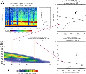
Fig. 6. (A) Earlinet lidar at Leipzig, Germany, showing the evolution of the major ash plume over Leipzig on 16 April 2010 (in red, 3–5 km height, 13:47–15:32 UTC) in terms of 1064 nm range-corrected (RC) lidar signal (arbitrary units), (B) WRF-Chem simulation from 10:00 to 16:00 UTC, and (C, D) vertical profiles at 11:00 and 14:00 UTC, respectively (adapted from Webley et al., 2012).
at 3.5 km a.s.l. Ansmann et al. (2010) showed from post-processed lidar data that the cloud was centred at 3.5 km and had ash concentrations around 900 µg m−3. The WRF-Chem
modelled magnitude (using the S2 size distribution) proved to be close to the lidar data, and the modelled vertical extent of the ash was well comparable to the lidar measurements.
5 The software
The software tool necessary to produce the input data to WRF-Chem simulates the movement of volcanic ash cloud, and SO2 is the PREP-CHEM-SRC emission tool (Freitas
et al., 2011). This system is coded using Fortran90 and C and requires Hierarchical Data Format (HDF) and Network Common Data Format (NetCDF) libraries. The desired grid configuration and emission inventories to provide emission fluxes and additional information are defined in a Fortran namelist file called “prep-chem-src.inp”. The software has been tested with GFortran, Intel and Portland Fortran com-pilers under the UNIX/LINUX operating system. Emissions output from the PREP-CHEM-SRC program are provided in separate intermediate binary data files for volcanic
emis-sions as well as anthropogenic emisemis-sions, biomass burning and GOCART aerosol background fields if so desired.
A utility program, convert emiss, is provided with the WRF-Chem model that converts these separate intermediate files from PREP-CHEM-SRC into WRF input data files. This utility program reads the volcanic emissions binary data file, and computes the vertical mass distribution and the sions for the volcanic ash size bin before populating the emis-sions input data arrays. The WRF-Chem model then reads the input data and then either re-computes the emissions based upon a new eruption height and vertical mass distribution provided as a WRF-Chem input parameter or uses the pre-scribed volcanic ash emissions.
6 Summary and conclusions
atmospheric transport of ash, subsequently 10 ash variables were added to WRF-Chem describing the typical bin size dis-tribution of the total ash during a volcanic eruption event.
The total ash is distributed into the model bins according to a typical particle distribution scheme, which is character-istic for each eruption type. During an eruption event, the ash is distributed in an umbrella-shaped vertical distribution plume above the volcano. Eruption source parameters have been compiled from historic eruptions (Mastin et al., 2009); the source parameters are characteristic for certain eruption types, and have been assigned to 1535 volcanoes worldwide. The parameters were implemented as a look-up table in the WRF-Chem PREP-CHEM-SRC emission tool. The data in-clude injection heights and the duration of an event, and rep-resent the best initial assessment of the type and size of fu-ture eruptions. In addition to ash, volcanic SO2sources were
added from the AEROCOM program. Alternatively to the AEROCOM dataset, SO2 was implemented in WRF-Chem
by distributing SO2in an umbrella-shaped plume in similar a
fashion to the ash. The SO2initial mass is also estimated as
a first guess.
This implementation offers opportunities for the opera-tional community to use this tool for prediction of hazardous evens. WRF-Chem results in mass concentrations of ash, which are useful for ash advisories; most offline Lagrangian models describe the particle trajectory, and additional as-sumptions are needed to derive mass concentrations of ash. Additionally, scientists may try to improve their understand-ing of the interaction of volcanic aerosols with radiation and microphysics. We plan to test WRF-Chem for near-real-time experimental WRF-Chem volcanic ash emission forecasts for modelling domains within the Anchorage Volcanic Ash Advisory Center (http://vaac.arh.noaa.gov/). Once the mete-orological source and boundary fields are created, a WRF-Chem run with 10 ash particle size bins takes about 25 min using 64 2.6 GHz AMD Opteron processors, and a modelling domain with a 12 km horizontal resolution, 300 by 300 hori-zontal grid cells (3600 km×3600 km), and 50 vertical levels; the experimental runs calculate gravitational settling and wet deposition of ash.
Studies with different volcanic ash source models are in progress to test the sensitivity of the various eruption source parameters. Initial model runs of the 1989 Redoubt erup-tion and the 2010 Eyjafjallaj¨okull eruperup-tion showed promis-ing results. The distal ash cloud durpromis-ing the 2010 event was well comparable with satellite remote sensing data and li-dar measurements. Grell and Baklanov (2011) indicate that the vertical motion fields in the atmosphere may exhibit very large variabilities, which are especially challenging to simu-late with offline models. WRF-Chem resulted in a vertically confined ash cloud, which compared well with the shown li-dar measurements from Leipzig. Obviously, the initial ash particle size distribution and the associated mass are critical for the downwind ash concentrations. Devenish et al. (2012) have shown the sensitivity of the size of the ash particles for
modelling concentrations of the distal ash clouds from Eyjaf-jallaj¨okull in May 2010. Long distance ash transport is deter-mined by the total amount of the emitted fine ash generated by explosive fragmentation at the source and by particle ag-gregation. So far there is no parameterization of aggregation of volcanic ash particles included in WRF-Chem, although Sparks et al. (1997) state that most of the fine ash typically aggregates. In most cases we would overestimate concen-trations of fine ash afar from the erupting volcano without considering the factors which determine the efficiency of ag-gregation. However, typically there exists high uncertainty in the particle size distribution and the fine ash at the source, and most ash dispersion models reduce aggregation errors by assuming a smaller fine ash fraction when defining the erup-tion source parameters used for the models. Future work is needed and online models such as WRF-Chem will facilitate the implementation of parameterization schemes for aggre-gation of ash particles as described by Costa et al. (2010).
Acknowledgements. This publication results in part from research
sponsored by the Cooperative Institute for Alaska Research with funds from the National Oceanic and Atmospheric Administration under cooperative agreement NA08OAR4320751 with the Uni-versity of Alaska. The authors acknowledge support from the US Air Force Weather Agency, the University of Alaska Arctic Region Supercomputing Center, and the NOAA Health of the Atmosphere Program. Saulo R. Freitas acknowledges support of this work by CNPq (302696/2008-3). We would like to thank Larry Mastin and the anonymous reviewer for their comments.
Edited by: A. Stenke
References
Ackermann, I. J., Hass, H., Memmesheimer, M. , Ebel, A., Binkowski, F. S., and Shankar, U.: Modal aerosol dynamics model for Europe: Development and first applications, Atmos. Environ., 32, 2981–2999, doi:10.1016/S1352-2310(98)00006-5, 1998.
Ahmadov, R., McKeen, S. A., Robinson, A., Bahreini, R., Mid-dlebrook, A., de Gouw, J., Meagher, J., Hsie, E., Edgerton, E., Shaw, S., and Trainer, M.: A volatility basis set model for summertime secondary organic aerosols over the east-ern United States in 2006, J. Geophys. Res., 117, D06301, doi:10.1029/2011JD016831, 2012.
Albrecht, B. A.: Aerosols, cloud microphysics, and fractional cloudiness, Science, 245, 1227–1230, doi:10.1126/science.245.4923.1227, 1989.
Arason, P., Petersen, G. N., and Bjornsson, H.: Observations of the altitude of the volcanic plume during the eruption of Eyjafjal-laj¨okull, April–May 2010, Earth System Science Data, 3, 9–17, doi:10.5194/essd-3-9-2011, 2011.
Barnard, J. C., Fast, J. D., Paredes-Miranda, G., Arnott, W. P., and Laskin, A.: Technical Note: Evaluation of the WRF-Chem “Aerosol Chemical to Aerosol Optical Properties” Module using data from the MILAGRO campaign, Atmos. Chem. Phys., 10, 7325–7340, doi:10.5194/acp-10-7325-2010, 2010.
Bonadonna, C., Mayberry, G. C., Calder, E. S., Sparks, R. S. J., Choux, C., Jackson, A. M., Lejeune, A. M., Loughlin, S. C., Norton, G. E., Rose, W. I., Ryan, G., and Young, S. R.: Tephra fallout in the eruption of Soufri`ere Hills Volcano, Montserrat, in: The eruption of Soufri`ere Hills Volcano, Montser-rat, from 1995 to 1999, edited by: Druitt, T. H. and Koke-laar, B. P., Geological Society of London, London, 483–516, doi:10.1144/GSL.MEM.2002.021.01.22, 2002.
Bonadonna, C. and Houghton, B. F.: Total grain-size distribution and volume of tephrafall deposits, B. Volcanol., 67, 441–456, doi:10.1007/s00445-004-0386-2, 2005.
Bulletin of the Global Volcanism Network (BVGN): Weekly report of Puyehue-Cord´on Caulle volcano, available at: http://www.volcano.si.edu/world/volcano.cfm?vnum=1507-15= &volpage=weekly, last access: 9 July 2012, 1–7 June 2011. Carey, S. N. and Sigurdsson, H.: Influence of particle aggregation
on deposition of distal tephra from the May 18, 1980, eruption of Mount St. Helens volcano, J. Geophys. Res., 87, 7061–7072, 1982.
Casadevall, T. J.: The 1989/1990 eruption of Redoubt Volcano Alaska: impacts on aircraft operations, J. Volcanol. Geoth. Res., 62, 301–316, 1994.
Chapman, E. G., Gustafson Jr., W. I., Easter, R. C., Barnard, J. C., Ghan, S. J., Pekour, M. S., and Fast, J. D.: Coupling aerosol-cloud-radiative processes in the WRF-Chem model: Investigat-ing the radiative impact of elevated point sources, Atmos. Chem. Phys., 9, 945–964, doi:10.5194/acp-9-945-2009, 2009.
Chen, F. and Dudhia, J.: Coupling an advanced land-surface/hydrology model with the Penn State/NCAR MM5 modeling system. Part I: Model description and implemen-tation, Mon. Weather Rev., 129, 569–585, doi:10.1175/1520-0493(2001)129<0587:CAALSH>2.0.CO;2, 2001.
Chin, M., Ginoux, P., Kinne, S., Holben, B. N., Duncan, B. N., Martin, R. V., Logan, J., Higurashi, A., and Nakajima, T.: Tropospheric aerosol optical thickness from the GOCART model and comparisons with satellite and sunphotometer mea-surements, J. Atmos. Sci., 59, 461–483, doi:10.1175/1520-0469(2002)059<0461:TAOTFT>2.0.CO;2, 2002.
Chou, M. D., Suarez, M. J. , Ho, C. H., Yan, M. M. H., and Lee, K. T.: Parameterizations for cloud overlapping and shortwave single-scattering properties for use in general circu-lation and cloud ensemble models, J. Climate, 11, 202–214, doi:10.1175/1520-0442(1998)011<0202:PFCOAS>2.0.CO;2, 1998.
Costa, A., Folch, A., and Macedonio, G.: A model for wet aggregation of ash particles in volcanic plumes and clouds: 1. Theoretical formulation, J. Geophys. Res., 115, B09201, doi:10.1029/2009JB007175, 2010.
Devenish, B. J., Francis, P. N., Johnson, B. T., Sparks, R. S. J., and Thomson, D. J.: Sensitivity analysis of dispersion modeling of volcanic ash from Eyjafjallaj¨okull in May 2010, J. Geophys. Res., 117, D00U21, doi:10.1029/2011JD016782, 2012. Diehl, T.: A global inventory of volcanic SO2emissions for
hind-cast scenarios, available at: http://www-lscedods.cea.fr/aerocom/ AEROCOM HC/, last access: 28 March 2013, 2009.
Diehl, T., Heil, A., Chin, M., Pan, X., Streets, D., Schultz, M., and Kinne, S.: Anthropogenic, biomass burning, and volcanic emissions of black carbon, organic carbon, and SO2from 1980 to 2010 for hindcast model experiments, Atmos. Chem. Phys. Discuss., 12, 24895–24954, doi:10.5194/acpd-12-24895-2012, 2012.
Durant, A. J. and Rose, W. I.: Sedimentological constraints on hydrometeor-enhanced particle deposition: 1992 Eruptions of Crater Peak, Alaska, J. Volcanol. Geoth. Res., 186, 40–59, doi:10.1016/j.jvolgeores.2009.02.004, 2009.
Durant, A. J., Rose, W. I., Sarna-Wojcicki, A. M., Carey, S., and Volentik, A. C.: Hydrometeor-enhanced tephra sed-imentation: Constraints from the 18 May 1980 eruption of Mount St. Helens (USA), J. Geophys. Res., 114, B03204, doi:10.1029/2008JB005756, 2009.
Fast, J. D., Gustafson Jr., W. I., Easter, R. C., Zaveri, R. A., Barnard, J. C., Chapman, E. G., Grell, G. A., and Peckham, S. E.: Evolution of ozone, particulates, and aerosol direct radia-tive forcing in the vicinity of Houston using a fully coupled meteorology-chemistry-aerosol model, J. Geophys. Res., 111, D21305, doi:10.1029/2005JD006721, 2006.
Freitas, S. R., Longo, K. M., Silva Dias, M. A. F., Chatfield, R., Silva Dias, P., Artaxo, P., Andreae, M. O., Grell, G., Rodrigues, L. F., Fazenda, A., and Panetta, J.: The Coupled Aerosol and Tracer Transport model to the Brazilian developments on the Re-gional Atmospheric Modeling System (CATT-BRAMS) – Part 1: Model description and evaluation, Atmos. Chem. Phys., 9, 2843– 2861, doi:10.5194/acp-9-2843-2009, 2009.
Freitas, S. R., Longo, K. M., Alonso, M. F., Pirre, M., Marecal, V., Grell, G., Stockler, R., Mello, R. F., and S´anchez G´acita, M.: PREP-CHEM-SRC – 1.0: a preprocessor of trace gas and aerosol emission fields for regional and global atmospheric chemistry models, Geosci. Model Dev., 4, 419–433, doi:10.5194/gmd-4-419-2011, 2011.
Grell, G., Freitas, S. R., Stuefer, M., and Fast, J.: Inclusion of biomass burning in WRF-Chem: impact of wildfires on weather forecasts, Atmos. Chem. Phys., 11, 5289–5303, doi:10.5194/acp-11-5289-2011, 2011a.
Grell, G. A. and Baklanov, A.: Integrated Modeling for Forecasting Weather and Air Quality: A Call for Fully Coupled Approaches, Atmos. Environ., 45, 6845–6851, doi:10.1016/j.atmosenv.2011.01.017, 2011.
Grell, G. A. and D´ev´enyi, D.: A generalized approach to pa-rameterizing convection combining ensemble and data as-similation techniques, Geophys. Res. Lett., 29, 38-1–38-4, doi:10.1029/2002GL015311, 2002.
Grell, G. A., Fast, J., Gustafson, W. I., Peckham, S. E., McKeen, S. A., Salzmann, M., and Freitas, S.: On-Line Chemistry within WRF: Description and Evaluation of a State-of-the-Art Multi-scale Air Quality and Weather Prediction Model, in: Integrated Systems of Meso-Meteorological and Chemical Transport Mod-els, edited by: Baklanov, A., Mahura, A., and Sokhi, R., Springer, 2011b.
Gudmundsson, M. T., Pedersen, R., Vogfj¨ord, K., Thorbjarnard´ottir, B., Jakobsd´ottir, S., and Roberts, M. J.: Eruptions of Eyjafjal-laj¨okull Volcano, Iceland, Eos T. Am. Geophys. Un., 91, 190– 191, doi:10.1029/2010EO210002, 2010.
Gustafson Jr., W. I., Chapman, E. G., Ghan, S. J., Easter, R. C., and Fast, J. D.: Impact on Modeled Cloud Characteristics Dueto Simpli?ed Treatment of Uniform Cloud Condensation Nu-clei During NEAQS 2004, Geophys. Res. Lett., 34, L19809, doi:10.1029/2007GL030021, 2007.
Hong, S. Y., Dudhia, J., and Chen, S. H.: A revised approach to ice-microphysical processes for the bulk parameterization of cloud and precipitation, Mon. Weather Rev., 132, 103–120, doi:10.1175/1520-0493(2004)132<0103:ARATIM>2.0.CO;2, 2004.
Iacono, M. J., Delamere, J. S., Mlawer, E. J., Shephard, M. W., Clough, S. A., and Collins, W. D.: Radiative forcing by long-lived greenhouse gases: Calculations with the AER radiative transfer models, J. Geophys. Res., 113, D13103, doi:10.1029/2008JD009944, 2008.
Janji´c, Z. I.: Nonsingular implantation of the Mellor–Yamada level 2.5 scheme in the NCEP mesomodel, NOAA/NWS/NCEP Office Note 437, 61 pp., 2002.
Lathem, T. L., Kumar,P., Nenes, A., Dufek, J., Sokolik, I. N., Trail, M., and Russell, A.: Hygroscopic properties of volcanic ash, Geophys. Res. Lett., 38, L11802, doi:10.1029/2011GL047298, 2011.
Mastin, L., Guffanti, M., Servranckx, R., Webley, P., Barsotti, S., Dean, K., Durant, A., Ewert, J., Neri, A., and Rose, W.: A multi-disciplinary effort to assign realistic source parameters to models of volcanic ash-cloud transport and dispersion during eruptions, J. Volcanol. Geoth. Res., 186, 10–21, 2009.
McCormick, M. P., Thomason, L. W., and Trepte, C. R.: Atmo-spheric effects of the Mt. Pinatubo eruption, Nature, 373, 399– 404, doi:10.1038/373399a0, 1995.
Miller, T. P. and Chouet, B. A.: The 1989-1990 eruptions of Re-doubt volcano: an introduction, in: The 1989-1990 eruptions of Redoubt Volcano, Alaska, edited by: Miller, T. P. and Chouet, B. A., J. Volcanol. Geoth. Res., 62, 1–10, doi:10.1016/0377-0273(94)90025-6, 1994.
Mlawer, E. J., Taubman, S. J., Brown, P. D., Iacono, M. J., and Clough, S. A.: Radiative transfer for inhomogeneous atmo-sphere: RRTM, a validated correlated-k model for the longwave, J. Geophys. Res., 102, 16663–16682, doi:10.1029/97JD00237, 1997.
Pruppacher, H. R. and Klett, J. D.: Microphysics of Clouds and Pre-cipitation, Second edition, Kluwer Academic Publishers, Dor-drecht, The Netherlands, 954 pp., 1997.
Rose, W. I., Kostinski, A., and Kelley, L.: Real-time C-band radar observations of 1992 eruption clouds from Crater Peak, Mount Spurr Volcano, Alaska: in: The 1992 eruptions of Crater Peak vent, Mount Spurr Volcano, Alaska, edited by: Keith, T. E. C., U.S. Geological Survey Bulletin B 2139, 19–26, 1995.
Rose, W. I., Self, S., Murrow, P. J., Ernst, G. J., Bonadonna C., and Durant, A. J.: Pyroclastic fall deposit from the October 14, 1974 eruption of Fuego Volcano, Guatemala, B. Volcanol., 70, 1043– 1067, 2007.
Salzmann, M.: WRF-Chem/KPP Coupler (WKC) for WRF V3, Users’ and Developers Guide v2.0, Princeton University, Prince-ton, NJ, USA, 2008.
Schell, B., Ackermann, I. J., Hass, H., Binkowski, F. S., and Ebel, A.: Modeling the formation of secondary organic aerosol within a comprehensive air quality modeling system, J. Geophys. Res., 106, 28275–28293, doi:10.1029/2001JD000384, 2001.
Scollo, S., Del Carlo, P., and Coltelli, M.: Tephra fallout of 2001 Etna flank eruption: Analysis of the deposit and plume disper-sion, J. Volcanol. Geoth. Res., 160, 147–164, 2007.
Scott, W. E. and McGimsey, R. G.: Character, mass, distribution, and origin of tephra-fall deposits of the 1989–1990 eruption of Redoubt Volcano, south-central Alaska, in: The 1989–1990 Eruptions of Redoubt Volcano, Alaska, edited by: Miller, T. P. and Chouet, B. A., J. Volcanol. Geoth. Res., 62, 251–272, doi:10.1016/0377-0273(94)90036-1, 1994.
Shrivastava, M., Fast, J., Easter, R., Gustafson Jr., W. I., Zaveri, R. A., Jimenez, J. L., Saide, P., and Hodzic, A.: Modeling organic aerosols in a megacity: comparison of simple and complex rep-resentations of the volatility basis set approach, Atmos. Chem. Phys., 11, 6639–6662, doi:10.5194/acp-11-6639-2011, 2011. Skamarock, W. C., Klemp, J. B., Dudhia, J., Gill, D. O., Barker,
D., Duda, M. G., Huang, X.-Y., and Wang, W.: A Description of the Advanced Research WRF Version 3, NCAR Technical Note TN-468+STR, 113 pp., 2008.
Sparks, R. S. J., Bursik, M. I., Carey, S. N., Gilbert, J. S., Glaze, L. S., Sigurdsson, H., and Woods, A. W.: Volcanic Plumes. John Wiley and Sons, Sussex, UK, 574 pp., 1997.
Stockwell, W. R., Middleton, P., Chang, J. S., and Tang, X.: The sec-ond generation regional acid deposition model chemical mech-anism for regional air quality modeling, J. Geophys. Res., 95, 16343–16367, doi:10.1029/JD095iD10p16343, 1990.
Twomey, S.: The Influence of Pollution on the Shortwave Albedo of Clouds. J. Atmos. Sci., 34, 1149–1152, doi:10.1175/1520-0469(1977)034<1149:TIOPOT>2.0.CO;2, 1977.
Webley, P. W. and Mastin, L. G.: Improved Prediction and track-ing of Volcanic Ash clouds, in: Special Issue on Volcanic Ash Clouds, edited by: Mastin, L. and Webley, P., J. Volcanol. Geoth. Res., 186, 1–9, doi:10.1016/j.jvolgeores.2008.10.022, 2009. Webley, P. W., Steensen, T., Stuefer, M., Grell, G. A., Freitas, S.,
and Pavolonis, M.: Analyzing the Eyjafjallaj¨okull 2010 erup-tion using satellite remote sensing, lidar and WRF-Chem dis-persion and tracking model, J. Geophys. Res., 117, D00U26, doi:10.1029/2011JD016817, 2012.
World Meteorological Organization (WMO): Workshop on Ash Dispersal forecast and civil aviation: model definition document, available at: http://www.unige.ch/sciences/terre/mineral/CERG/ Workshop/results/Model-Document-Geneva10.pdf (last access: 16 April 2011), 2010.
Zaveri, R. A. and Peters, L. R.: A new lumped structure photochem-ical mechanism for large-scale applications, J. Geophys. Res., 104, 30387–30415, doi:10.1029/1999JD900876, 1999.