Geosci. Model Dev., 6, 2135–2152, 2013 www.geosci-model-dev.net/6/2135/2013/ doi:10.5194/gmd-6-2135-2013
© Author(s) 2013. CC Attribution 3.0 License.
Geoscientific
Model Development
Open Access
Accuracy of the zeroth- and second-order shallow-ice
approximation – numerical and theoretical results
J. Ahlkrona1,2, N. Kirchner2,3, and P. Lötstedt1
1Division of Scientific Computing, Department of Information Technology, Uppsala University, Uppsala, Sweden 2Bolin Centre for Climate Research, Stockholm University, Stockholm, Sweden
3Department of Physical Geography and Quaternary Geology, Stockholm University, Stockholm, Sweden
Correspondence to: J. Ahlkrona ([email protected])
Received: 20 June 2013 – Published in Geosci. Model Dev. Discuss.: 7 August 2013 Revised: 31 October 2013 – Accepted: 14 November 2013 – Published: 19 December 2013
Abstract. In ice sheet modelling, the shallow-ice approxi-mation (SIA) and second-order shallow-ice approxiapproxi-mation (SOSIA) schemes are approaches to approximate the solu-tion of the full Stokes equasolu-tions governing ice sheet dynam-ics. This is done by writing the solution to the full Stokes equations as an asymptotic expansion in the aspect ratio, i.e. the quotient between a characteristic height and a char-acteristic length of the ice sheet. SIA retains the zeroth-order terms and SOSIA the zeroth-, first-, and second-order terms in the expansion. Here, we evaluate the order of accuracy of SIA and SOSIA by numerically solving a two-dimensional model problem for different values of, and comparing the solutions with a finite element solution to the full Stokes equations obtained from Elmer/Ice. The SIA and SOSIA so-lutions are also derived analytically for the model problem. For decreasing, the computed errors in SIA and SOSIA de-crease, but not always in the expected way. Moreover, they depend critically on a parameter introduced to avoid singu-larities in Glen’s flow law in the ice model. This is because the assumptions behind the SIA and SOSIA neglect a thick, high-viscosity boundary layer near the ice surface. The sen-sitivity to the parameter is explained by the analytical solu-tions. As a verification of the comparison technique, the SIA and SOSIA solutions for a fluid with Newtonian rheology are compared to the solutions by Elmer/Ice, with results agreeing very well with theory.
1 Introduction
The cryosphere is an important part of the climate sys-tem, and includes, among other features, the Greenland Ice Sheet and the Antarctic Ice Sheet. With a volume of about 3×10⁷km3, these two ice sheets represent the largest com-ponent of the cryosphere, and store about 77 % of the global freshwater. Cryospheric research, and specifically, ice sheet modelling, is a vibrant discipline which receives much scien-tific, political and societal attention because of its relevance for predictions of the future sea level rise in a warming world (Solomon et al., 2007).
more restricted than it is today. Yet, because of challenging applications such as palaeoglacial simulations or uncertainty quantifications, they have not lost their relevance, and a large portion of ice sheet simulations is still performed with SIA codes or higher-order approximations today.
In this paper we investigate the order of accuracy and va-lidity of a higher-order extension to the SIA; the second-order shallow-ice approximation (SOSIA). In the process we also study the accuracy of the classical SIA. The SIA was constructed in the 1970s and 1980s by Fowler and Larson (1978), Hutter (1983) and Morland (1984). The derivation is based on scaling and asymptotic series expansion in terms of the aspect ratio,, which expresses the shallowness of an ice sheet. In the SIA, only the zeroth-order terms are kept. In the end of the 1990s, the second-order shallow-ice approxima-tion (SOSIA) was derived by Baral (1999) and Baral et al. (2001), pushing the series expansion to second order in with the objective of including dynamics not captured by the SIA. Computing a solution with SOSIA can be viewed as two steps in an iteration. First the SIA solution is determined, and then the SOSIA solution. A fully iterative algorithm is devel-oped in Souˇcek and Martinec (2008), based on an asymptotic expansion in.
The SOSIA is thus a higher-order model based on the same theory as the SIA, and is almost as computationally cheap as the SIA. The scaling assumptions underlying the SOSIA (and the SIA as derived in Baral, 1999; Baral et al., 2001; Greve, 1997) do, however, neglect a high-viscosity boundary layer near the ice surface. This boundary layer is thick (Ahlkrona et al., 2013), and other scaling assumptions by Johnson and McMeeking (1984) and Schoof and Hindmarsh (2010) are more appropriate than the classical SIA scalings (Ahlkrona et al., 2013). This calls for a proper analysis of the accuracy of the SOSIA equations, and also an investigation of the true order of accuracy of the SIA. The boundary layer is associ-ated with the non-linear rheology of ice. There is no bound-ary layer in a Newtonian fluid at the upper surface and the scaling assumptions made to derive the SIA and SOSIA are valid for the whole fluid.
Our analysis is based on analytical solutions of the SOSIA (and SIA) as well as numerical solutions of SIA, SOSIA and the full Stokes equations when there is no sliding at the ice base. Ultimately, it is of interest to assess under which cir-cumstances the SOSIA model can be regarded as a signif-icant improvement on the SIA at low computational costs. The SOSIA, as described in Baral et al. (2001), has to our knowledge never been implemented before this study, most likely because the second-order expressions are long and te-dious to code. The SOSIA was applied by Mangeney and Califano (1998) for Newtonian, anisotropic ice, and recently was applied by Egholm et al. (2011) – not, however, in its pure form, but in a depth-averaged, iterative scheme.
The outline of this paper is as follows: Sect. 2 is de-voted to a summary of the general equations pertaining to ice dynamics, and to their zeroth-, first-, and second-order
approximations. Recent works by Ahlkrona et al. (2013) and Kirchner et al. (2011) allow us to keep this presentation to a minimum. Sect. 3 describes the model problem which we focus on throughout the paper: a two-dimensional flow over a bumpy bed. In Sect. 4 an analytical SOSIA solution for this model problem is presented and discussed, extending previous work by Baral (1999) and Baral et al. (2001). The solution is compared to the SIA and SOSIA solutions of a Newtonian fluid. In Sect. 5 we implement the SOSIA nu-merically and compute the accuracy of both the SIA and the SOSIA by comparing their solutions with the solution ob-tained with Elmer/ICE (Gagliardini et al., 2013), for vary-ing. The same computations are repeated for a Newtonian fluid to verify that the comparison technique is reliable. In both Sects. 4 and 5 we compare our results with the theory in Schoof and Hindmarsh (2010) and investigate the effect of an extra parameter,σres, which is necessary due to the neglect of the boundary layer at the surface. The paper concludes with a discussion in Sect. 6.
2 Derivation of the zeroth- and second-order shallow-ice approximation
2.1 The exact equations
Ice sheet flow is commonly described using concepts from continuum mechanics, materials science, and thermodynam-ics, which allow for the formulation of the spatio–temporal evolution of ice masses as an initial boundary value problem, with free boundaries. Ice flow is momentum, mass, and in-ternal energy conserving. As we will only study isothermal flow, the equations regarding energy are not described here. The equations for balance of mass and momentum are
0=divv, (1)
ρv˙= −∇p+divTD+ρg, (2)
whereρis the density,vthe velocity field,TDthe deviatoric stress tensor andggravitational acceleration. The deviatoric stress tensor,TD, and the Cauchy stress tensor,T are related byT = −pI+TD, wherepis the pressure. The acceleration term,v˙ – which is the material time derivative of the veloc-ity in Eq. (2) – is very small and is therefore neglected in glaciological applications. The resulting equations are called the Stokes equations, or in glaciology rather the full Stokes equations. Velocity and stress are related by the constitutive equation,
D=A(T0)f (σ )TD, (3)
in glaciology called Glen’s flow law. The strain rate tensorD is defined as(∇v+(∇v)∗)/2, where∗denotes transpose and
J. Ahlkrona et al.: The second-order shallow-ice approximation 2137 function,f, is defined byf (σ )=σn−1, where we letnbe
equal to the standard value 3. Its argument,σ, the effective stress, is the square root of the second invariant ofTD, and is defined by
σ2=1
2tr(T
D)2=(tD
xz)2+(tyzD)2+(txyD)2 (4) +1
2
(txxD)2+(tyyD)2+(tzzD)2.
Here, tijD (i, j=x, y, z) are the components of TD in a Cartesian coordinate system where thezaxis is pointing in the opposite direction of gravity. We refer totxxD,tyyD andtzzD as normal deviatoric stresses, totxzD (=txz) andtyzD (=tyz) as vertical shear stresses and totxyD (=txy) as the horizon-tal plane shear stress. As the creep response function
de-pends on the effective stress, ice is a non-Newtonian fluid with viscosity, η, given by 1/η=2A(T0)f (σ ). This non-linearity makes the ice flow simulations a computationally heavy task. The computations are simpler in a Newtonian fluid withn=1. Thenf =1 and the relation betweenDand TDin Eq. (3) is linear for a constantT0.
To complete the system, boundary conditions are imposed at the ice base and ice surface. At the impermeable ice base, the velocity satisfies no slip conditions on a rigid bedrock, giving the condition
v=0. (5)
The ice surface is assumed to be stress-free,
T ·n=0. (6)
Herenis the outward-pointing normal vector of the ice surface. In the time-dependent case, a transport equation for the ice surface elevation is solved, where the velocity field enters as coefficients and the accumulation or ablation en-ters as a forcing. The equation for the height of the free ice surfaceh(x, y, t )is
∂h ∂t +vx
∂h ∂x+vy
∂h
∂y−vz=as, (7)
wherevx,vyandvzare the velocity components andasis the accumulation/ablation function.
2.2 Shallow-ice approximations
Here we briefly describe how the SIA and the SOSIA are derived from the exact, full Stokes equations by scaling and perturbation expansions. We exemplify the procedure by the momentum balance Eq. (2). We follow the scalings presented in Baral (1999), Baral et al. (2001), and Greve (1997), as these are the ones most commonly used today for deriving the SIA, and also those used to go further and arrive at the SOSIA equations. These scalings are
(x, y)= [L](x,˜ y),˜
z= [H]˜z,
t=([L]/[VL])t,˜ p=ρg[H] ˜p,
(txzD, tyzD, σ )=ρg[H](t˜D
xz,t˜yzD,σ ),˜ (txxD, tyyD, txyD, tzzD)=2ρg[H](t˜D
xx,t˜ D yy,t˜
D xy,t˜
D zz),
(vx, vy)= [VL](v˜x,v˜y), vz= [VH] ˜vz,
= [H]/[L] = [VH]/[VL],
F = [VL]2/g[L], (8)
where the aspect ratio,, has been introduced. The dimen-sionless quantities are denoted by tilde and are assumed to be of the order of magnitudeO(1). They are multiplied by typ-ical values of height,[H], length,[L], vertical velocity[VH] and horizontal velocity, [VL], where[H] [L] so that the aspect ratio,, is small. The scaling reflects that the vertical shear stresses are assumed to dominate over the normal devi-atoric and normal shear stresses, and that this dominance is stronger the more shallow the ice sheet is. Also, the horizon-tal velocity is assumed to dominate over the vertical velocity,
[VH] [VL].
The scalings Eq. (8) are inserted into the equations and a perturbation expansion is performed, i.e. the dimensionless variables,q˜, are expanded in a power series as
˜
q= ˜q(0)+q˜(1)+2q˜(2)+. . . (9) Collecting terms of equal order in gives rise to a hier-archy of models, called the SIA for zeroth order in , the FOSIA (first-order shallow-ice approximation) for first order in, and SOSIA for second order. The momentum balance Eq. (2) (in component form), for the SIA model is
0= −∂p˜(0) ∂x˜ +
∂t˜D xz(0)
∂z˜ , (10a)
0= −∂p˜(0) ∂y˜ +
∂t˜D yz(0)
∂z˜ , (10b)
1= −∂p˜(0)
∂z˜ . (10c)
For the FOSIA, it is
0= −∂p˜(1) ∂x˜ +
∂t˜D xz(1)
∂z˜ , (11a)
0= −∂p˜(1) ∂y˜ +
∂t˜D yz(1)
∂z˜ , (11b)
0= −∂p˜(1)
For the SOSIA, it is
0= −∂p˜(2) ∂x˜ +
∂t˜D xz(2) ∂z˜ +
∂t˜D xx(0) ∂x˜ +
∂t˜D xy(0)
∂y˜ , (12a)
0= −∂p˜(2) ∂y˜ +
∂t˜D yz(2) ∂z˜ +
∂t˜D xy(0) ∂x˜ +
∂t˜D yy(0)
∂y˜ , (12b)
0= −∂p˜(2) ∂z˜ +
∂t˜D xz(0) ∂x˜ +
∂t˜D yz(0) ∂y˜ +
∂t˜D zz(0)
∂z˜ . (12c)
Note that there are no other stress components besides the vertical shear stress in the zeroth-order equations. This is the main reason why higher-order models are becoming increas-ingly popular:txx(D 0),tyy(D 0),tzz(D0)andtxy(D 0)are important in the coupling to ice shelves and in ice streams and ice stream shear margins.
The boundary conditions are also expanded. The stress-free condition thatT ·n=0 corresponds to
p(0)=0, (13)
txz(D 0)=0, (14)
in zeroth order, and
p(2)= −tzz(D0), (15)
txz(D 2)= −(tzz(D0)−txx(D 0))∂h
∂x, (16)
in second order. The no-slip condition will for the problem studied in this paper reduce tovx=vy=vz=0 for both ze-roth and second order. The stress componentstxx(D 0),tyy(D 0), tzz(D0) andtxy(D 0) do not require explicit boundary conditions but will be determined at the boundaries implicitly through the stress–strain relation.
Integrating Eq. (10c) in the vertical direction and using the boundary condition that the pressure is zero at the ice sur-face gives an explicit expression for the pressure. Inserting the pressure in Eqs. (10a) and (10b), integrating and using the stress-free condition again yields simple expressions for the vertical shear stresses. The shear stresses are sufficient to obtain the zeroth-order (SIA) velocities by integration of the stress–strain rate relation Eq. (3); see Sect. 4 for the outcome of this standard procedure. Once the zeroth-order solution is available, it can be used to solve the FOSIA, and subse-quently the SOSIA equations by the same method.
Just like the SIA, the FOSIA only contains the vertical shear stresses, but no normal deviatoric stress or horizon-tal plane shear stress. However, the FOSIA does account for first-order boundary effects and forcings that cannot be repre-sented in SIA (Baral, 1999). For the model problem that we study, the FOSIA solution is trivially zero, and the FOSIA will hence not be further discussed. It is in the SOSIA that the normal deviatoric stresses and the horizontal plane shear stresses are present for the first time, suggesting that more complex ice dynamical behaviour can be captured by the
SOSIA than by the SIA. The SOSIA is computationally in-expensive compared to many other higher-order models, be-cause the equations can be solved without a coupling of vari-ables in a system of linear equations.
2.3 Boundary layer treatment
The SIA and the SOSIA are both based on the same scaling arguments in Eq. (8), where it is assumed, in addition to the ice body being shallow, that the dominating stress compo-nent is vertical shear stress and that the velocity compocompo-nents in the horizontal plane dominate over the vertical velocity. These assumptions are not valid in a number of well-known situations, including fast sliding at the ice-bedrock interface (as in for example ice streams), or at the ice divide where the ice flows mainly downwards. Where fast sliding occurs it is common to use other scaling arguments, such as e.g. the shelfy stream approximation in MacAyeal (1992). Dif-ferent traction numbers representing difDif-ferent sliding speeds combined with other scalings are introduced in Schoof and Hindmarsh (2010).
Another region where the SIA scalings break down is in a boundary layer near the entire ice surface, which develops when there is a bumpy bed due to the non-linear rheology of ice (Ahlkrona et al., 2013). Johnson and McMeeking (1984) made the first attempt to derive a solution for the bound-ary layer by matched asymptotics, rescaling the pressure and stress components in the boundary layer. This allows for all stress components to influence the dynamics near the ice sur-face. By theoretical analysis they found the boundary layer thickness to be O(13). Schoof and Hindmarsh (2010)
ex-tended the boundary layer theory by including the degree of slip at the bed in the expansion, and pushing it to sec-ond order. In the case of slow sliding, the rescaling of the pressure and stress components in the boundary layer in two dimensions is as in Johnson and McMeeking (1984); Ahlkrona et al. (2013) and in Schoof and Hindmarsh (2010). Using their traction numberλ=1/3for the conditions at the bedrock:
p=1/3ρg[H] ˜p,
tDxz=4/3ρg[H] ˜tDxz, (17)
(txxD, tzzD)=4/3ρg[H](t˜D xx,t˜
D zz).
By numerically solving the full Stokes equations, Ahlkrona et al. (2013) essentially confirmed the appropriate-ness of these rescalings for the problem described in Sect. 3. In fluid dynamics, boundary layers are usually assumed to be thin, but as found in Ahlkrona et al. (2013), they may be thick and indistinct at the ice surface (depending on), and this needs to be considered in model development.
J. Ahlkrona et al.: The second-order shallow-ice approximation 2139 and Baral et al. (2001) indeed dismiss it as too complicated
and use the scalings in Eq. (8) for the entire ice sheet in the derivation of the SIA and SOSIA. This, in combination with the fact that the rheology of ice is singular and non-linear, does introduce complications that need to be reme-died. The singularity arises from the fact that the creep re-sponse function is zero for zero effective stress, i.e.f (0)=0. This means that the viscosity is infinite where the effective stress is zero. By the shallow-ice scalings Eq. (8), the normal and horizontal plane shear stresstxxD,tyyD,tzzD,txyD in Eq. (4) are neglected such thatf (σ(0))=σ(20)=t
2 xz(0)+t
2
yz(0). Thus the (zeroth-order) effective stress and the creep response func-tion are zero wherever the zeroth-order vertical shear stresses are zero, which is at the entire ice surface (Baral, 1999; Baral et al., 2001; Greve, 1997). In reality, normal deviatoric stresses (and depending on the situation, horizontal plane shear stresses) develop, implying non-zero effective stress at the ice surface except for a few points.
As SIA is the zeroth-order expansion, it can be derived us-ing several different scalus-ing arguments. Therefore, it is not very sensitive to the neglect of normal and horizontal plane shear stress in the boundary layer. Indeed, the computation of the SIA solution does not include the reciprocal of the creep response function (except for in the normal deviatoric stress), and the fact that the zeroth-order effective stress is zero at the entire surface does not imply singularities in the velocity field, pressure, or shear stress. The SOSIA is how-ever bound to be more sensitive. When pushing the asymp-totic expansions to second order, the creep response function of the zeroth-order effective stress does occur in the denom-inator. To remedy this, an extra parameter,σres, is used in Baral (1999) and Baral et al. (2001), to regularise the prob-lem, following earlier suggestions by Lliboutry (1969) and Colbeck and Evans (1973). This parameter, which we will call the finite viscosity parameter σres, is added to f as: f (σ )=σ2+σres2 (see e.g. Colbeck and Evans, 1973). Non-singular creep functions of non-additive structure have been proposed by e.g. Lliboutry (1969). The question of the appro-priateness of modifying the material law instead of rescaling the variables in the boundary layer immediately arises. As al-ready mentioned, the singularities do not affect SIA. Hence, in practice σres is not needed in the SIA, but the solution will not be accurate to the order predicted by the theory in Baral (1999) and Baral et al. (2001). It is unclear whether the SOSIA will be an improvement on SIA, because of the neglect of the special boundary layer dynamics. Moreover, there is no obvious way to choose the value of the finite-viscosity parameter. In Baral et al. (2001), σres=
√
109 is used for the Greenland Ice Sheet, but with no explanation of this choice. In Sect. 5, we will investigate how to chooseσres, how accurate the SIA is, and whether the SOSIA really is an improvement on the SIA.
J. Ahlkrona et al.: The second order shallow ice approximation 5
As SIA is the zeroth order expansion it can be derived us-ing several different scalus-ing arguments. Therefore it is not very sensitive to the neglect of normal and horizontal plane shear stress in the boundary layer. Indeed, the computation of the SIA solution does not include the reciprocal of the creep response function (except for in the normal deviatoric stress), and the fact that the zeroth order effective stress is zero at the entire surface does not imply singularities in the velocity field, pressure, or shear stress. The SOSIA is how-ever bound to be more sensitive. When pushing the asymp-totic expansions to second order, the creep response func-tion of the zeroth order effective stress does occur in the
de-nominator. To remedy this, an extra parameter,σres, is used
in Baral (1999) and Baral et al. (2001), to regularize the problem, following earlier suggestions by Lliboutry (1969) and Colbeck and Evans (1973). This parameter, which we will call thefinite viscosity parameterσres, is added tofas:
f(σ) =σ2+σ2
res(see e.g. Colbeck and Evans, 1973).
Non-singular creep functions of non-additive structure have been proposed by e.g. Lliboutry (1969). The question of the appro-priateness in modifying the material law instead of rescaling the variables in the boundary layer immediately arises. As al-ready mentioned, the singularities do not affect SIA. Hence,
in practiceσres is not needed in the SIA, but the solution
will not be accurate to the order predicted by the theory in Baral (1999) and Baral et al. (2001). It is unclear whether the SOSIA will be an improvement of SIA, because of the neglect of the special boundary layer dynamics. Moreover, there is no obvious way to choose the value of the finite vis-cosity parameter. In Baral et al. (2001),σres=
√
109is used
for the Greenland ice sheet, but with no explanation of this
choice. In Sect. 5, we will investigate how to chooseσres,
how accurate the SIA is, and whether the SOSIA really is an improvement of the SIA.
3 Model problem – ice flow over a bumpy bed
Throughout this paper we will consider the model problem described in this section. It is a slight modification of the problem studied in the ISMIP-HOM benchmark experiment B (Pattyn et al., 2008). As in Pattyn et al. (2008), we in-vestigate a diagnostic, isothermal 2-D-problem for ice flow over an inclined, bumpy bed. The ice surface is fixed, pe-riodic boundary conditions are applied and no-slip condi-tions are imposed at the base, see Fig. 1. The rate factor
A is10−16Pa−3a−1, ice density is the standard value of
910 kg m−3, and accumulation and ablation are neglected.
The mean ice thickness,[H], is 1000mand the ice surface,
h, and ice base,b, are given by
h(x) =−xtan(α), b(x) =h−[H] +µ[H] sin
2π Lx
.
(18)
α
L
[H]
z
x
Fig. 1.Model set-up showing the basal topography and the ice sur-face. The ice flows down-slope in the positivex-direction.
The ice base is smooth, thus avoiding additional difficulties with SIA and SOSIA for a bedrock with less regularity. The
amplitude of the bumps isµ[H]and the inclination angle
of the surface slope isα. The typical horizontal extent of
the problem equals the wavelength of the sinusoidal bumps,
i.e. L= [H]/m. The wavelengthL of the bumps is
var-ied while[H]is kept constant, which corresponds to varying
. As shown in Ahlkrona et al. (2013), and as can be seen
for instance by non-dimensionalising the ice surface and ice
bed, the surface slope angleαshould be proportional toe.g.
arctaninstead ofα= 0.5owhich was used in the
ISMIP-HOM benchmark. The bump amplitudeµshould be
indepen-dent of. In our numerical experiments we will useµ= 0.5
andµ= 0.1.
4 Analytical solutions for the SIA and the SOSIA
For a deeper understanding, we now compute analytical so-lutions for the second order field variablestxz(2),px(2)and
vx(2), and also give the zeroth order expressions for
com-pleteness. Note that for the 2-D casevy=tyyD =txyD = 0. The
second orderzvelocity is excluded for brevity of
presenta-tion, since it follows from the mass balance in the same way for all orders.
4.1 General solution
The following expressions (Eqs. 19–24) hold, not only for our model problem, but for all isothermal, 2-D problems with no-slip conditions at the base and without higher or-der boundary terms. Generalising to 3-D, including higher order boundary terms, and sliding, is straightforward. The well-known zeroth order expressions, denoted by subscript
Fig. 1. Model set-up showing the basal topography and the ice sur-face. The ice flows downslope in the positivexdirection.
3 Model problem – ice flow over a bumpy bed
Throughout this paper we will consider the model problem described in this section. It is a slight modification of the problem studied in the ISMIP-HOM benchmark experiment B (Pattyn et al., 2008). As in Pattyn et al. (2008), we in-vestigate a diagnostic, isothermal 2-D problem for ice flow over an inclined, bumpy bed. The ice surface is fixed, pe-riodic boundary conditions are applied and no-slip condi-tions are imposed at the base (see Fig. 1). The rate factor
A is 10−16Pa−3a−1, ice density is the standard value of 910 kg m−3, and accumulation and ablation are neglected. The mean ice thickness,[H], is 1000 m and the ice surface, h, and ice base,b, are given by
h(x)= −xtan(α),
b(x)=h− [H] +µ[H]sin 2
π L x
. (18)
The ice base is smooth, thus avoiding additional difficul-ties with SIA and SOSIA in modelling a bedrock with less regularity. The amplitude of the bumps isµ[H]and the incli-nation angle of the surface slope isα. The typical horizontal extent of the problem equals the wavelength of the sinusoidal bumps, i.e.L= [H]/m. The wavelengthLof the bumps is varied while[H]is kept constant, which corresponds to vary-ing.
4 Analytical solutions for the SIA and the SOSIA For a deeper understanding, we now compute analytical so-lutions for the second-order field variablestxz(2),px(2) and vx(2), and also give the zeroth-order expressions for com-pleteness. Note that for the 2-D case,vy=tyyD =txyD =0. The second-orderzvelocity is excluded for the sake of brevity, since it follows from the mass balance in the same way for all orders.
4.1 General solution
The following expressions (Eqs. 19–24) hold not only for our model problem, but also for all isothermal, 2-D problems with no-slip conditions at the base and without higher-order boundary terms. Generalising to three-dimensionality, in-cluding higher-order boundary terms and sliding, is straight-forward. The well-known zeroth-order expressions, denoted by subscript(0), for shear stress (cf. Eq. 10) and velocity are txz(D 0)= −ρg∂h(0)
∂x (h(0)−z), (19)
vx(0)= −2ρg ∂h(0)
∂x z Z
b(0)
Af (σ(0))(h(0)−z0)dz0, (20)
withvx(0)=0 atb(0), cf. Eq. (5). In order to computetxz(D2) from Eq. (12) we need the zeroth-order normal deviatoric stresses (and depending on the situation, horizontal plane shear stress), which are not computed when applying only the zeroth-order approximation, as they are not needed for the zeroth-order velocities. The normal deviatoric stress in thexdirection is given directly by the stress–strain relation in Baral et al. (2001) and Greve (1997):
txx(D 0)= 1 Af (σ(0))
∂vx(0)
∂x . (21)
Note that txxD = −tzzD in the 2-D case. The shear stress, pressure and the horizontal velocity are obtained from the horizontal momentum balance, vertical momentum balance and stress–strain relation, respectively, where they occur in derivatives.
It is customary to vertically integrate the SIA equations in order to avoid having to solve for the variables numerically. This is also convenient for the SOSIA. In Baral et al. (2001), the vertical integration is carried out for the shear stresses and the pressure only, and the resulting expressions are presented in Eqs. (22) and (23) (with misprints in Baral et al., 2001, cor-rected). Going beyond the results of Baral et al. (2001), we derive here also the second-order velocity,vx(2), in Eq. (24), computed from the stress–strain relation and boundary con-ditions at the base:
2p(2)=ρg 1
2 h(0)−z
2∂2h(0) ∂x2
+ρg h(0)−z ∂h
(0) ∂x
2
+tzz(D0), (22)
2txz(D 2)=ρg ∂ ∂x
1
6(z−h(0)) 3∂2h(0)
∂x2 h(0)
−ρg ∂ ∂x
1
2 z−h(0)
2∂h(0) ∂x
2!
− ∂
∂x h(0)
Z
z
tzz(D0)dz0+ ∂ ∂x
h(0)
Z
z
txx(D 0)dz0, (23)
2vx(2)= − ∂ ∂x
z Z
b(0)
vz(0)dz+6A z Z
b(0)
(txz(D 0))22txz(D2)dz0
+2A z Z
b(0)
txz(D0)(txx(D 0))2dz0+2σres2 A z Z
b(0)
2txz(D2)dz0. (24)
Equations (22)–(24) yield explicit expressions for second-order variables.
4.2 Solution for the model problem
For the geometry in Sect. 3, we have computed the integrals and derivatives in these expressions and thus obtained an-alytical solutions to the SOSIA. To avoid infinite viscosity, we have followed the suggested regularisation in Baral et al. (2001), i.e. adding a constant to the creep response function, f (σ )=σ2+σres2 . The solutions are expressed in terms of the inclination angle of the ice surfaceα, relative amplitudeµ, finite-viscosity parameter,σres, and wavelengthL. In the Ap-pendix A the same solutions are expressed in a more general form. By Eq. (19), the zeroth-order shear stress for the model problem is
txz(D0)= −ρgtan(α) (xtan(α)+z) . (25) The zeroth-order velocity in Eq. (20) is given by
vx(0)=2ρgAtan(α)
(ρg)2tan2(α)
4 (26)
[H]4(1−µsin(2π x/L))4−(xtan(α)+z)4
+ σ
2 res 2
[H]2(1−µsin(2π x/L))2−(xtan(α)+z)2
.
J. Ahlkrona et al.: The second-order shallow-ice approximation 2141 continuing to second order. To calculate second-order shear
stress and velocity, the zeroth-order normal deviatoric stress in Eq. (21) is needed. It is given for the model problem by txx(D 0)= −2ρgtan2(α) (xtan(α)+z)
−4π L ρg[H]
2µtan(α)cos(2π x/L) (1−µsin(2π x/L)) (xtan(α)+z)2tan2(α)+σres
ρg 2
(27)
· tan2(α)[H]2(1−µsin(2π x/L))2+
σ res ρg
2! .
Having calculatedtxx(D 0), the second-order shear stress is computed from Eq. (23) as
2txz(D2)=3ρgtan3(α)(xtan(α)+z)
+4ρg[H]22π L µtan
2(α)(1−µsin(2π x/L))cos(2π x/L) tan2(α)(xtan(α)+z)2+ σres2
(ρg)2
·
[H]2tan2(α) (1−µsin(2π x/L))2+ σ
2 res (ρg)2
−4(ρg)
2[H]2 σres
2π L
2 µ
3[H]2(1−µsin(2π x/L))2µcos2(2π x/L)tan2(α) + [H]2(1−µsin(2π x/L))3sin(2π x/L)tan2(α)
+ σ
2 res (ρg)2
µcos2(2π x/L)+(1−µsin(2π x/L))
sin(2π x/L))
·arctan
ρgtan(α)(xtan(α)+z) σres
. (28) An explicit dependence onLis introduced in Eqs. (27)–(28), and hence on the aspect ratio. Also, Eqs. (27) and (28) de-pend onα,µandσres. Intxx(D 0),σresappears in the denomi-nator, preventing singularities from occurring at the ice sur-face whenzis equal toh= −xtan(α); see Eq. (27). In the second-order shear stress in Eq. (28),σres is both in the nu-merator and the denominator. The second-order shear stress is dominated by the last term, i.e. by the last five lines in Eq. (28).
Having calculatedtxx(D 0) andtxz(D2), the second-order ve-locity can be derived from Eq. (24). The expression for the second-order solution is very long and is included in the Ap-pendix A for the interested reader. In fact it behaves similarly to the second-order shear stress, whereσres appears both in the numerator and the denominator. Remember that to get the full second-order solution, the zeroth- and second-order con-tributions should be added together asvx=vx(0)+2vx(2) (the first-order solution is zero for our model problem). The extra term arising from the finite-viscosity law in vx(0) in
Eq. (26) is quite large, and thus the SOSIA velocity does not allow too large aσres. The SOSIA shear stress is not as sensitive to largeσres, since the zeroth-order shear stress in Eq. (25) does not contain any terms from the finite-viscosity law. Both the second-order shear stress correction and veloc-ity correction are, however, very sensitive to too small aσres. Note that all terms involvingσres in Eqs. (27), (28), and (A6) in the Appendix A are pre-multiplied withµ; thus, the importance ofσresdecays whenµdecreases. This is consis-tent with the fact that the boundary layer near the ice surface disappears whenµ=0 (Ahlkrona et al., 2013).
4.3 Choices ofσresand impact on scalings
In order for any scaling relations (Eq. 8 or 17) to hold, tan(α) should vary linearly with , e.g. tan(α)=, and µshould be independent of(Ahlkrona et al., 2013). Note, however, that the scaling relations were derived in a context where the creep response function was not modified by an additional finite-viscosity parameter. We now discuss howσres, intro-duced in an a posteriori fashion, can be chosen such that com-patibility with either the classical SIA scalings in Eq. (8) or the ones in Eq. (17) is achieved.
4.3.1 Choosing aσresconsistent with the classical
SIA-scalings
If we choose the finite-viscosity parameter,σres, to vary in the same way as the effective stress is assumed to (linearly with), the SIA and SOSIA solutions fulfil the scaling rela-tions Eq. (8) that they are derived from. Inserting tan(α)=, σres=Cσρg[H] and the scaled variables in Eq. (8) into Eqs. (25)–(28) yields
txz(D0)= −ρg[H](x˜+ ˜z), (29)
vx(0)=A[H](ρg[H])33 1
2(1−µsin(2πx))˜ 4−1
2(x˜+ ˜z) 4
+Cσ2
(1−µsin(2πx))˜ 2−(x˜+ ˜z)2 , (30)
txx(D 0)= −ρg[H]2 2 (x˜+ ˜z)2+C2
σ
(x˜+ ˜z)(x˜+ ˜z)2+Cσ2
−2π µcos(2πx) (˜ 1−µsin(2πx))˜ (1−µsin(2πx))˜ +Cσ2, (31)
2txz(D 2)=ρg[H]3
3(x˜+ ˜z)
+8π µ
(1−µsin(2πx))˜ cos(2πx)˜ (1−µsin(2πx))˜ 2+Cσ2 (x˜+ ˜z)2+C2
−16π2 µ Cσ
3µ (1−µsin(2πx))˜ 2cos2(2πx)˜
+(1−µsin(2πx))˜ 3sin(2πx)˜
+Cσ2µcos2(2πx)˜ +(1−µsin(2πx))˜ sin(2πx)˜
·arctan x˜+ ˜z
Cσ
, (32)
where Cσ is a constant and x˜ and z˜ are the non-dimensionalisedx andzcoordinates in Eq. (8). The expres-sions in Eqs. (29)–(32) only depend on geometry, material constants, andCσ. In line with Eq. (8),txz(D0)is pre-multiplied byρg[H],txx(D 0)is pre-multiplied byρg[H]2and2txz(D2) is pre-multiplied byρg[H]3. Note that the multiplying fac-tor in vx(0) is A[H](ρg[H])33 as in Blatter (1995) and Schoof and Hindmarsh (2010). In the same manner, the ana-lytical solution forvz(0)(which is not given here for brevity of presentation) is multiplied byA[H](ρg[H])34.
4.3.2 Choosing aσresconsistent with boundary layer
theory
We know that the scaling relations Eq. (17) from Schoof and Hindmarsh (2010) (slightly rearranged) are more correct than the classical scaling relations in Eq. (8) (Ahlkrona et al., 2013; Schoof and Hindmarsh, 2010; Johnson and McMeek-ing, 1984), and thatσresis merely a parameter introduced to address this problem when using Eq. (8). However, we show now that instead of settingσres=Cσρg[H], withCσ con-stant, we can chooseCσsuch that the field variables fulfil the scaling relations in Eq. (17) rather than Eq. (8).
Near the ice surface, σ is dominated by txxD (Ahlkrona et al., 2013; Schoof and Hindmarsh, 2010) and the creep re-sponse function satisfiesf (σ )≈(txxD)2in 2-D. In the SOSIA model, txxD is neglected in the creep response, and instead f (σ )=σres2 at the ice surface. This is a consequence of the asymptotic expansion of the solution and of equating terms of equal order. Hence, Cσ in σres=Cσρg[H] should be such thatσres=txxD in the upper boundary layer. Let Cσ= Cγγ and insert it into Eq. (31). Sincex˜+ ˜z=0 at the sur-face, we havetxxD ∼2/2γ ∼σres∼1+γ and consequently thatγ=1/3. ThentxxD ∼4/3 in the boundary layer as de-rived in Eq. (3.108) in Schoof and Hindmarsh (2010). Out-side the boundary layer in Eq. (31), when x˜+ ˜z=O(1), txxD ∼2as expected from the SOSIA equations. By replac-ingCσ byCγγ in the expression fortxxD in Eq. (31), insert-ingσres=txxD andx˜+ ˜z=0, solving forCγ and finally ignor-ing terms dependignor-ing on, we find thatCγ is approximated by
Cγ3=4π µcos(2πx)(˜ 1−µsin(2πx))˜ 2. (33) ThusCγ decreases with decreasing bump amplitude only depend on the geometry and is of O(1). Due to the
assumptions made when obtaining Eq. (33), it cannot be used directly to determine Cγ, but gives an understanding of its behaviour which we will recognise in our numerical experi-ments.
The first correction term applied to the SIA solutiontxz(D0) in Eq. (29) is2txz(D 2) in Eq. (32). WithCσ =Cγ1/3, at the ice surface and outside the boundary layer
2txz(D 2)∼7/3, x˜+ ˜z=0, (34a) 2txz(D 2)∼8/3, x˜+ ˜z=O(1), (34b) in agreement with the second terms in the expansions in Eqs. (3.108) and (3.73) in Schoof and Hindmarsh (2010). The velocity componentvx(0) in Eq. (4.11) is ofO(3)for everywhere in the ice. The first correction termvx(2) in the Appendix A depends in the same way astxz(D2) onσres−1 out-side the boundary layer andσres−2close to the ice surface.
In our numerical experiments we will apply bothσres= Cσρg[H]andσres=Cγρg[H]4/3, whereCσ andCγ are constants.
4.4 A Newtonian fluid
For comparison, we derive the asymptotic expansions for a Newtonian fluid withn=1 in Glen’s flow law in Eq. (3) us-ing the same techniques as for the ice model withn=3 and the same model problem in Sect. 3. The shear stress is inde-pendent of the flow law in Eq. (19), and the zeroth-order term is the same as in Eq. (25):
txz(D0)= −ρgtan(α) (xtan(α)+z) . (35) Sincef (σ(0))=1 in Eq. (20) there is no need to introduce σres, and the expression for the zeroth-order velocity is sim-plified compared to Eq. (26):
vx(0)=ρgAtan(α)
·([H]2(1−µsin(2π x/L))2−(xtan(α)+z)2). (36) This expression is equal to the contribution by the constant part of the creep function in Eq. (26). Also the lowest order term in the normal deviatoric stress in Eq. (21) is simplified whenn=1:
txx(D 0)= −2ρgtan(α)2(xtan(α)+z) (37)
−4π L ρg[H]
2µtan(α)cos(2π x/L) (1−µsin(2π x/L)) .
This formula is similar to the formula fortxx(D 0)whenn=
3 in Eq. (27). The second-order shear stress is obtained by Eq. (23):
2txz(D 2)=3ρgtan3(α)(xtan(α)+z) −4ρgµ[H]2tan(α)
2π L
2
J. Ahlkrona et al.: The second-order shallow-ice approximation 2143
·(1−µsin(2π x/L)) (xtan(α)+z) (38)
−4ρgµ2[H]2tan(α) 2
π L
2
cos2(2π x/L)(xtan(α)+z) +4ρgµ[H]2tan2(α)2π
L cos(2π x/L) (1−µsin(2π x/L)) . The first term is the same as in Eq. (28) in the non-Newtonian case, while the rest of the expression is simpler and does not include any terms withσres or arctan. Neither Eq. (37) nor (38) is singular for anyx andz, as txx(D 0) and txz(D 2)are withσres=0 in Eq. (27) and (28).
Since xtan(α)+z∼ [H] and with tan(α)∼ we have through Eqs. (35) and (36) that txz(D0)∼[H] and vx(0)∼ [H]2. Hence, for the zeroth-order velocity in the z direc-tion,
vz(0)= − z Z
b(0)
∂vx(0) ∂x dz
0∼
3[H]2, (39)
and for the second-order velocity inxdirection,
2vx(D2)= − ∂ ∂x
z Z
b(0)
vz(0)dz0+ z Z
b(0)
2txz(2)dz0∼2[H]2. (40)
The scaling in Eq. (37) is such thattxx(D 0)∼2[H], and in Eq. (38), such that2txz(D2)∼3[H]. These scalings are all in agreement with the assumptions made in Eq. (8) in the derivations of the shallow-ice approximations.
5 Numerical computation of the accuracy of SIA and SOSIA
In this section, we compute the SIA and SOSIA solutions for the problem described in Sect. 3, and compute the solutions’ accuracy by comparing them with a full Stokes solution. All our results presented in this section regard the accuracy for thexvelocity,vx, and shear stress,txzD. The normal deviatoric stressestxxD andtzzDare not calculated to second order, since this is not necessary in order to obtain the velocity field. The vertical velocity is also excluded, as it follows directly from the mass balance, which is the same for all orders.
5.1 Method
We are interested in the order of accuracy, i.e. how the error in SIA and SOSIA varies with. For this purpose we perform repeated simulations usingL=10, 20, 40, 80, 160, 320, 640, 1280, 2560, 5120, and 10 240 km while keepingHconstant; this is equivalent to varying the aspect ratio between 9.77×
10−5and 0.1. We do this in order to investigate the accuracy of shallow-ice approximations in the limit→0.
The SOSIA Eqs. (19)–(24) are implemented in MATLAB and our implementation follows the standard in SImulation
COde for POLythermal Ice Sheets (SICOPOLIS) (Greve, 1995). Finite differences are used on a staggered grid in or-der to avoid having oscillatory solutions with the same wave-length as small multiples of the grid size. The velocities, horizontal volume fluxes, vertical shear stresses and the hor-izontal derivatives of the bedrock topography and the ice-surface topography are defined in between the grid points. All other quantities are defined at grid points. When a quan-tity is needed at a point where it is not defined, linear inter-polation is used. To ensure that the grid points coincide with physical boundaries, aσ transformation is used (Greve and Blatter, 2009; Greve, 1995). Central differences are applied when possible; otherwise one-sided differences are used. In-tegrals are computed by the trapezoidal method if the inte-grand and the integral are defined at the same points. Other-wise, the midpoint rule is used.
The full Stokes solution that we use for comparison is ob-tained using the finite-element code Elmer/Ice (Gagliardini et al., 2013). The same mesh with the nodes on vertical lines was used for SIA, SOSIA and in Elmer/Ice. We use a mesh fine enough to keep the relative numerical error below 10−4 for both the velocity and shear stress. This error can be seen in some of the figures below, but as the mesh is refined it decreases even more. Even though the singular behaviour of the viscosity does not introduce singularities in the field vari-ables in the full Stokes setting, an extra parameter, the critical shear rateγ˙o, is introduced in Elmer/Ice in order to treat nu-merical instabilities at low stress (Råback et al., 2013), occur-ring e.g. near the ice surface in the shear stress. The critical shear rate is a lower bound for the shear rateγ˙, which is re-lated to the effective stress byγ˙=p2t r(D2)=2d=2Aσ3. We have used γ˙o=10−10 throughout the simulations. For large aspect ratios there is noγ˙o which suppresses the nu-merical instabilities in the shear stress without altering the velocity.
The accuracy is measured in terms of the relative error de-fined by
||qx,full Stokes−qx,SIA/SOSIA||2
||qx,full Stokes||2
, (41)
whereq isvx ortxzD and|| · ||2denotes theL2norm defined by
||q||2=
v u u t
1 V
Z
q2d, (42)
whereVis the area of. The integral in Eq. (42) is com-puted on a discrete grid using the trapezoidal rule.
5.2 Results
We know from our analytical solutions in Sect. 4.3 that the SOSIA solution is very sensitive to the parameterσres. There-fore, we experiment with different values of and ways of set-tingσres.
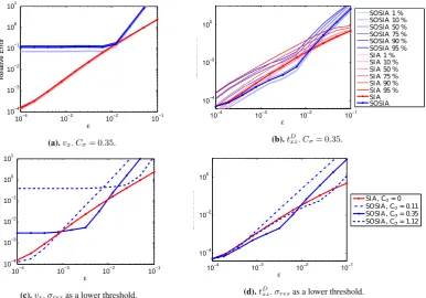
Our analytical solutions suggest that if the scaling rela-tions used to derive the SOSIA were correct,σresshould vary withasCσρg[H],Cσ being a constant. This relationship is used in Fig. 2a and b, showing the accuracy of the SIA and SOSIA solution for a bumpy bed with relative bump am-plitudeµ=0.5. The SIA solution for the horizontal velocity component isvx(0) in Eq. (26) withCσ=0, since a finite-viscosity law is unnecessary in this case. The SOSIA solution is computed forCσ equal to 0.35.
5.2.1 Accuracy of the SIA
We start by analysing the error in SIA. According to classi-cal SIA theory in Baral (1999), Baral et al. (2001), and Greve (1997), the SIA relative error should be ofO(2). However, we know from Ahlkrona et al. (2013) that the scalings used in Schoof and Hindmarsh (2010) are more correct than the classical SIA scalings. The asymptotic expansions in Schoof and Hindmarsh (2010) yield the same zeroth-order solution as the SIA, but the correction terms are different. The rela-tive error in the velocity is estimated by the first neglected term in the expansions ofvx in Eqs. (3.73) and (3.108) in Schoof and Hindmarsh (2010) and is of order 4/3 in the boundary layer and 5/3 outside the layer. The estimated slope, log(error)/log(), of the relative SIA error using all values in Fig. 2a (thick red line with nodes) is 1.43, which is between the theoretical rates in Schoof and Hindmarsh (2010). Similarly, the relative error in the SIA solution of txz(D 0)should, according to Eqs. (3.108) and (3.73) in Schoof and Hindmarsh (2010) and Eqs. (29) and (34), be4/3in the boundary layer and5/3outside it. This is in good agreement with the slope of the relative error in Fig. 2b, which is 1.38. 5.2.2 Accuracy of the SOSIA:σres=Cσρg[H]
We now move to analysing the SOSIA error in Fig. 2a and b (thick blue line with nodes). If the classical SIA theory were correct, SOSIA would in principle be much more accurate than SIA for sufficiently small. Clearly this is not the case in Fig. 2a and b. In addition to computing the SOSIA solu-tion withCσ=0.35, we also triedCσ =0.11 andCσ =1.12, with no improvement in accuracy.
The SOSIA is thus not a correction to the SIA with σres=Cσρg[H] andCσ constant. This is because the scal-ing relations in Eq. (8) are not correct for the thick boundary layer near the ice surface (which will domi-nate in the global error). Since the scaling relations do hold below this layer (Ahlkrona et al., 2013; Schoof and Hindmarsh, 2010; Johnson and McMeeking, 1984), one
would like to know if the SOSIA solution is more accu-rate further down in the ice. To investigate this, we com-pute the accuracy of SIA and SOSIA at horizontal layers at 0.01[H],0.5[H],0.75[H],0.9[H]and 0.95[H]mean height above the ice base; the result is included in Fig. 2a and b (the thin red and blue lines). The accuracy of the SOSIA velocity is slightly higher-deeper in the ice for small, but even there the SOSIA is less accurate than SIA. The shear stress is more accurate deeper in the ice for both SIA and SOSIA.
5.2.3 Accuracy of the SOSIA:σresas a lower threshold
The SOSIA solution is very sensitive toσres, and the differ-ent choices ofCσ yield very different results. To limit the sensitivity ofσres, we can choose to use it only where the ef-fective stress is too small. We therefore experiment withσres as a lower bound on the effective stress, viz.:
σ=max(σ(0), σres). (43)
Figure 2c and d show the error using this approach when Cσ =0.11, 0.35 and 1.12. The SOSIA velocity error de-creases considerably, and there are now aspect ratios for which SOSIA is more accurate than SIA whenCσ =0.35. The stress txzD is not largely affected. We have also com-puted the accuracy of SOSIA in layers throughout the ice, in the same way as in Fig. 2a and b. For the velocity there is a significant change for small aspect ratios. At 0.01[H]
mean height over the ice surface the SOSIA velocity solu-tion is more accurate than the SIA solusolu-tion for all aspect ra-tios smaller than 10−2. For the deviatoric shear stress, the layer-wise error is very similar to what is shown in Fig. 2b.
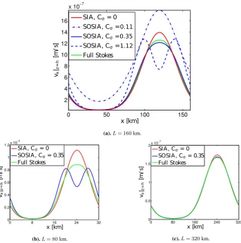
The error of the velocity for small aspect ratios is mainly due to the term on the third line of Eq. (26). It is an extra term in the zeroth-order velocity in SOSIA introduced by the use of a finite-viscosity law. This error is reduced by usingσres as a lower threshold and it is the most influential near the ice surface where the scaling relations do not hold and where the zeroth-order shear stress and therefore the zeroth-order effective stress is zero. This explains why the error decreases further down in the ice. Since there is no such zeroth-order term in the vertical shear stress, it is not affected by this type of error. In fact, for small aspect ratios, even an extremely largeσres does not cause a large error in the second-order shear stress. The stress is thus less sensitive to the handling of σres, which can be seen in Figs. 2a–d. The zeroth-order term involvingσresis dominant ifCσis too large and results in the velocity being too high overall (see Fig. 3a) whereCσ =1.12 and=1/160.
J. Ahlkrona et al.: The second-order shallow-ice approximationJ. Ahlkrona et al.: The second order shallow ice approximation 11 2145
10−4 10−3 10−2 10−1
10−4 10−3 10−2 10−1 100 101
ε
Relative Error
(a).vx.Cσ= 0.35.
10−4 10−3 10−2 10−1 10−4
10−2
100
ε
Relative
Error
SOSIA 1 % SOSIA 10 % SOSIA 50 % SOSIA 75 % SOSIA 90 % SOSIA 95 % SI A 1 % SI A 10 % SI A 50 % SI A 75 % SI A 90 % SI A 95 % SI A SOSIA
(b).tD
xz.Cσ= 0.35.
10−4 10−3 10−2 10−1
10−4 10−3 10−2 10−1 100 101
ε
Relative Error
(c).vx.σresas a lower threshold.
10−4 10−3 10−2 10−1 10−4
10−2
100
ε
Relative
Error SI A, Cσ= 0
SOSIA, Cσ= 0.11
SOSIA, Cσ= 0.35
SOSIA, Cσ= 1.12
(d).tD
xz.σresas a lower threshold.
Fig. 2.Relative error of horizontal velocityvxand vertical shear stresstxzDwithσres=Cσρg[H]for both SIA (red) and SOSIA (blue). Thick
lines show the error measured over the whole domain and the thin lines in the upper two panels show the errors measured over horizontal layers.
The relative error in vx decays as 2.81 in Fig. 2c for
≥1/320. This is the order of the next term in the ex-pansion. The reduction of the error ends when the term pro-portional to the constantσreswithCσ= 0.35in Eq. (26) be-comes important. The same observation is valid also for the SOSIA error in the vertical shear stress in Fig. 2d. The de-cay of the relative error for≥1/320is here2.51
before the reduction is damped by the constantσres. With the classical theory in Baral (1999) and Baral et al. (2001), the relative SOSIA error should beO(3). In practice, the larger aspect
ratios are of interest. Numerical errors are commonly of the order10−2
, which is higher than the model error in the SIA solution for aspect ratios smaller than3×10−3. For ice sheet
flow, aspect ratios smaller than10−3are seldom applicable.
5.2.4 Accuracy of the SOSIA: σres=Cγρg[H]4/3
and further adjustments
Figures 2c and 2d indicate that the optimal choice of Cσ might not be independent of the aspect ratio. Indeed, we found in Sect. 4 that if we choose σres as Cγρg[H]4/3 (whereCσ=Cγ1/3) the SOSIA correction terms are reme-died so that they are consistent with the scalings in
John-son and McMeeking (1984), Schoof and Hindmarsh (2010), and Ahlkrona et al. (2013), see Eq. (34). We can even go further in limiting the influence ofσresby only using it as a lower threshold in the computations where the creep re-sponse function is in the denominator (that is in the com-putation of the normal deviatoric, and normal shear stresses, see Eqs. (31) and (32)). The combined results of these two measures are shown in Figs. 4a and 4b. The SOSIA velocity and shear stress are now more accurate than SIA for all as-pect ratios smaller than10−2withC
γchosen to be3. The slope of the errors in Fig. 4 is almost equal for both SIA and SOSIA indicating that the order inin the remaining error is the same for both approximations. Using a different param-eter e.g.Cγ= 4results in SOSIA being more accurate than SIA for even larger aspect ratios, but on the other hand the improvement is no longer as significant. The parameterCγ depends on the geometry (see Eq. (33)) and is thus problem dependent and difficult to determine beforehand. Interesting to note is that there is no difference in accuracy of the ve-locity in the different layers through the ice. The accuracy of the deviatoric shear stress through the layers is distributed similarly to Fig. 2b.
Fig. 2. Relative error of horizontal velocityvxand vertical shear stresstxzD withσres=Cσρg[H]for both SIA (red) and SOSIA (blue). Thick lines show the error measured over the whole domain and the thin lines in the upper two panels show the errors measured over horizontal layers.
term in the second-order shear stress, i.e. the last five lines in Eq. (28), or the last four lines in Eq. (32). As this term de-pends on(1−µsin(2π x/L)), it is largest atx=3L/4, and as it is pre-multiplied byµ/Cσ, it will in general decrease with increasingCσ and decrease with decreasing bump am-plitude. The error is attributed to the improper handling of the singularity in Glen’s flow law. At the pointx=3L/4 the effective stress is zero in both the SOSIA as well as in the full Stokes setting.
The relative error in vx decays at 2.81 in Fig. 2c for ≥1/320. This is the order of the next term in the ex-pansion. The reduction of the error ends when the term pro-portional to the constantσreswithCσ =0.35 in Eq. (26) be-comes important. The same observation is also valid for the SOSIA error in the vertical shear stress in Fig. 2d. The de-cay of the relative error for≥1/320 is here2.51before the reduction is damped by the constantσres. With the classical theory in Baral (1999) and Baral et al. (2001), the relative SOSIA error should beO(3). In practice, the larger aspect ratios are of interest. Numerical errors are commonly of the order 10−2, which is higher than the model error in the SIA solution for aspect ratios smaller than 3×10⁻³. For ice sheet flow, aspect ratios smaller than 10−3are seldom applicable.
5.2.4 Accuracy of the SOSIA:σres=Cγρg[H]4/3and
further adjustments
Figure 2c and d indicate that the optimal choice of Cσ might not be independent of the aspect ratio. Indeed, we found in Sect. 4 that if we choose σres as Cγρg[H]4/3 (whereCσ =Cγ1/3) the SOSIA correction terms are reme-died so that they are consistent with the scalings in Johnson and McMeeking (1984), Schoof and Hindmarsh (2010), and Ahlkrona et al. (2013); see Eq. (34). We can even go further in limiting the influence ofσres by only using it as a lower threshold in the computations where the creep response func-tion is in the denominator (that is in the computafunc-tion of the normal deviatoric, and normal shear stresses, see Eqs. 31 and 32). The combined results of these two measures are shown in Fig. 4a and b. The SOSIA velocity and shear stress are now more accurate than in SIA for all aspect ratios smaller than 10−2withC
12 J. Ahlkrona et al.: The second order shallow ice approximation
0 50 100 150
2 4 6 8 10 12 14 16
x 10−7
x [km] vx
|z=
h
[m
/s
]
SIA, Cσ= 0
SOSIA, Cσ=0.11
SOSIA, Cσ=0.35
SOSIA, Cσ=1.12
Full Stokes
(a).L= 160 km.
0 8 16 24 32
0 0.2 0.4 0.6 0.8 1 1.2 x 10⁻⁵
x [km] vx
|z=
h
[m
/s
]
SIA, Cσ= 0 SOSIA, Cσ= 0.35 Full Stokes
(b).L= 80 km.
0 80 160 240 320
0 0.5 1 1.5
2 x 10 −7
x [km] vx
|z=
h
[m
/s
]
SIA, Cσ= 0 SOSIA, Cσ= 0.35 Full Stokes
(c).L= 320 km.
Fig. 3.Surfacexvelocity for the full Stokes solution, the SIA and the SOSIA. For SOSIA,σres=Cσρg[H]is used as a lower threshold for
the effective stress.
5.2.5 Low bump amplitude
Here we investigate how the accuracy changes as the bump amplitude is decreased. There is a common perception that shallow ice approximations are more accurate for lower bump amplitudes. Also, we found in Sect. 4 that the terms involvingσresin the stresses and (Eqs. 31 and 32) and ve-locity Eq. (A8) were pre-multiplied with the relative bump amplitudeµ, suggesting that the influence ofσresdecreases with decreasing bump amplitude. We have applied the SIA and SOSIA forµ= 0.1(a bump amplitude of10% of mean ice thickness), and the result is illustrated in Fig. 4c and d. We setσresin the same way as in Fig. 4a and b but withCγ= 1.5 instead ofCγ= 3. Indeed, Eq. (33) shows thatCγdecreases withµ. There is a small improvement of the accuracy of SIA and SOSIA compared to the case whenµ= 0.5. For large aspect ratios of almost0.1there is a notable improvement in
both SIA and SOSIA, but at these large aspect ratios the er-rors are still very large and neither SIA nor SOSIA is a good model. An explanation of the lack of significant improvement for lower amplitudes is that even if the classical scalings in Eq. (8) do hold for a flat bed, the thick boundary layer where variables rescale develops very rapidly as a small bump is introduced (Ahlkrona et al., 2013). Note that for very small aspect ratios numerical errors are present, so that the error for SIA and SOSIA is not smaller than10−4. This causes a bend
in the curves in the lower left parts of Figs. 4c and 4d, but also in Figs. 2a–2b and 4a–4b.
5.3 Newtonian Fluid
As seen in Sect. 4.4, the classical SIA-scalings hold for a Newtonian rheology (n= 1). For a Newtonian fluid we therefore expect the error in the SIA and SOSIA to behave
Fig. 3. Surfacexvelocity for the full Stokes solution, the SIA and the SOSIA. For SOSIA,σres=Cσρg[H]is used as a lower threshold for the effective stress.
difference in the accuracy of the velocity for the different layers through the ice. The accuracy of the deviatoric shear stress through the layers is distributed similarly to how it is shown in Fig. 2b.
5.2.5 Low bump amplitude
Here we investigate how the accuracy changes as the bump amplitude is decreased. There is a common perception that shallow-ice approximations are more accurate for lower bump amplitudes. Also, we found in Sect. 4 that the terms involvingσresin the stresses and Eqs. ( 31 and 32) and the ve-locity in Eq. (A8) were pre-multiplied with the relative bump amplitudeµ, suggesting that the influence ofσres decreases with decreasing bump amplitude. We have applied the SIA and SOSIA forµ=0.1 (a bump amplitude of 10 % of mean ice thickness), and the result is illustrated in Fig. 4c and d. We setσresin the same way as in Fig. 4a and b but withCγ=1.5 instead ofCγ =3. Indeed, Eq. (33) shows thatCγ decreases withµ. There is a small improvement of the accuracy of SIA and SOSIA compared to the case whenµ=0.5. For large
aspect ratios of almost 0.1, there is a notable improvement in both SIA and SOSIA, but at these large aspect ratios the er-rors are still very large and neither SIA nor SOSIA is a good model. An explanation of the lack of significant improvement for lower amplitudes is that even if the classical scalings in Eq. (8) do hold for a flat bed, the thick boundary layer where variables rescale develops very rapidly as a small bump is introduced (Ahlkrona et al., 2013). Note that for very small aspect ratios, numerical errors are present, so that the error for SIA and SOSIA is not smaller than 10−4. This causes a bend in the curves in the lower left parts of Fig. 4c and d, but also in Figs. 2a–b and 4a–b.
5.3 Newtonian fluid
J. Ahlkrona et al.: The second-order shallow-ice approximationJ. Ahlkrona et al.: The second order shallow ice approximation 13 2147
10−4 10−3 10−2 10−1 10−4
10−3 10−2 10−1 100 101
ε
Relative Error
(a).vx.Cγ= 3.
10−4 10−3 10−2 10−1 10−4
10−2
100
ε
Relative
Error
SI A SOSIA
(b).tD xz.Cγ= 3.
10−4 10−3 10−2 10−1 10−4
10−3 10−2 10−1 100 101
ε
Relative Error
(c).vx. Low bump,Cγ= 1.5.
10−4 10−3 10−2 10−1
10−4
10−2 100
ε
Relative
Error
SIA SOSIA
(d).tD
xz. Low bump,Cγ= 1.5.
Fig. 4.Relative error of horizontal velocityvxand vertical shear stresstxzD for both SIA (red) and SOSIA (blue) forµ= 0.5andµ= 0.1.
σres=Cγρg[H]4/3is only used when needed in the denominator of the expressions.
10−3 10−2 10−1 10−4
10−3 10−2 10−1 100 101
ε
Relative Error
(a).vx. Newtonian fluid
10−3 10−2 10−1 10−4
10−2 100
ε
Relative Error
SIA SOSIA
(b).tD
xz. Newtonian fluid
Fig. 5.Relative error of zeroth order and second order horizontal velocityvxand vertical shear stresstxzDfor Newtonian fluid (n= 1).
as predicted in Baral et al., i.e. we expect the SIA error to be O(2)and the SOSIA error to beO(3). Verifying this con-firms that the methodology of all our numerical experiments in this paper is accurate. We measure the error for linear rhe-ology in the same way as for the non-Newtonian case. The results are shown in Fig. 5.
The relative error decreases much faster within Fig. 5
than in the non-Newtonian case. The error does not decrease below about10−4, but as in the non-Newtonian case the rea-son is the numerical errors in the Elmer/Ice and the SIA and SOSIA solutions which decrease with mesh size. These error are of the same order as in Sect. 5.2. A polynomial fit re-veals that the error in the SIA velocity isO(1.91)and in the
Fig. 4. Relative error of horizontal velocityvxand vertical shear stresstxzDfor both SIA (red) and SOSIA (blue) whenµ=0.5 andµ=0.1. σres=Cγρg[H]4/3is only used when needed in the denominator of the expressions.
J. Ahlkrona et al.: The second order shallow ice approximation 13
10−4 10−3 10−2 10−1
10−4 10−3 10−2 10−1 100 101
ε
Relative Error
(a).vx.Cγ= 3.
10−4 10−3 10−2 10−1 10−4
10−2 100
ε
Relative
Error
SI A SOSIA
(b).tDxz.Cγ= 3.
10−4 10−3 10−2 10−1
10−4 10−3 10−2 10−1 100 101
ε
Relative Error
(c).vx. Low bump,Cγ= 1.5.
10−4 10−3 10−2 10−1 10−4
10−2 100
ε
Relative
Error SIA
SOSIA
(d).tD
xz. Low bump,Cγ= 1.5.
Fig. 4.Relative error of horizontal velocityvxand vertical shear stresstxzD for both SIA (red) and SOSIA (blue) forµ= 0.5andµ= 0.1.
σres=Cγρg[H]4/3is only used when needed in the denominator of the expressions.
10−3 10−2 10−1
10−4 10−3 10−2 10−1 100 101
ε
Relative Error
(a).vx. Newtonian fluid
10−3 10−2 10−1
10−4 10−2 100
ε
Relative Error
SIA SOSIA
(b).tD
xz. Newtonian fluid
Fig. 5.Relative error of zeroth order and second order horizontal velocityvxand vertical shear stresstxzD for Newtonian fluid (n= 1).
as predicted in Baral et al., i.e. we expect the SIA error to be
O(2)and the SOSIA error to beO(3). Verifying this
con-firms that the methodology of all our numerical experiments in this paper is accurate. We measure the error for linear rhe-ology in the same way as for the non-Newtonian case. The results are shown in Fig. 5.
The relative error decreases much faster within Fig. 5 than in the non-Newtonian case. The error does not decrease below about10−4, but as in the non-Newtonian case the
rea-son is the numerical errors in the Elmer/Ice and the SIA and SOSIA solutions which decrease with mesh size. These error are of the same order as in Sect. 5.2. A polynomial fit re-veals that the error in the SIA velocity isO(1.91)and in the
Fig. 5. Relative error of zeroth- and second-order horizontal velocityvxand vertical shear stresstxzDfor Newtonian fluid (n=1).
in this paper is accurate. We measure the error for linear rhe-ology in the same way as for the non-Newtonian case. The results are shown in Fig. 5.
The relative error decreases much faster within Fig. 5 than in the non-Newtonian case. The error does not decrease below about 10−4, but, as in the non-Newtonian case, the reason is the numerical errors in the Elmer/Ice and the SIA and SOSIA solutions which decrease with mesh size. These errors are of the same order as in Sect. 5.2. A polynomial fit reveals that the error in the SIA velocity isO(1.91)and in the SIA shear stress it isO(1.93). The error in the SOSIA veloc-ity isO(3.14)and in the SOSIA shear stress it isO(3.23).
6 Discussion and conclusions
We have solved the SIA and the SOSIA equations both an-alytically and numerically, and determined and analysed the accuracy of the velocity,vx, and the shear stress,txzD, com-pared to the full Stokes equations. This was done for a model problem representing ice flow on a bumpy, sloping bed with no-slip conditions at the base, slightly modified from the ISMIP-HOM B benchmark set-up (Pattyn et al., 2008). The purpose was to determine whether the SOSIA is an improve-ment on the SIA which could be used in practice. We also wanted to show that a thick, high-viscosity boundary layer at the ice surface cannot be overlooked in higher-order asymp-totic expansions, and that it results in the SIA not being second-order accurate.
We know from Ahlkrona et al. (2013), Johnson and McMeeking (1984), and Schoof and Hindmarsh (2010) that the scaling arguments behind the SIA and SOSIA as stated in Baral et al. (2001) are not valid in the boundary layer near the surface. Consequently, the numerically computed accu-racy of the SIA is O(1.43) for the velocity and O(1.38) for the shear stress instead ofO(2), as expected from the classical SIA theory. Our results rather agree with the analy-sis in Schoof and Hindmarsh (2010), which predicts the ac-curacy of the SIA velocity and shear stress to beO(4/3) in the boundary layer andO(5/3)outside it. Our accuracy was measured over the whole domain including the boundary layer.
The neglect of the special boundary-layer dynamics in the classical SIA scalings results in singularities in the SOSIA field variables. To remedy this, the finite-viscosity parame-ter,σres, is added to the effective stress in the creep response function when computing the SOSIA. Both our analytical lutions and numerical experiments show that the SOSIA so-lution is very sensitive to this parameter. It can neither be chosen too large nor to small, since it appears in both the nu-merator and the denominator of the expressions. Too large aσres yields too high a velocity, especially for small aspect ratios. This is due to an extra order term in the zeroth-order velocity. This error is more important near the surface than further down in the ice. Ifσres is simply added to the creep response function asf (σ )=σ2+σres2 , the error is so large that the SOSIA velocity is less accurate than that of the SIA for all aspect ratios. If σres is instead used as a lower threshold for the effective stress, as in Eq. (43), the error is decreased so that there is a range of (quite small) aspect ratios for which SOSIA is an improvement on SIA. Further reduc-ing the effect ofσres – so that it is only used in the calcula-tions where singularities would arise otherwise – improves the accuracy even more. The shear stress is not as sensitive to too large aσres as the velocity is. Too small aσresyields errors in both the velocity and shear stress for large aspect ratios, due to excessive second-order corrections caused by the singularity in Glen’s flow law.
Depending on how we choose the value ofσres, the an-alytical expressions for the field variables conform with ei-ther the classical shallow-ice scalings that were used in the derivation, or with the scaling relations in Schoof and Hindmarsh (2010) which we know are accurate (Ahlkrona et al., 2013). For agreement with the classical SIA scalings we conclude that σres should be Cσρg[H] where Cσ is a constant. In order for the solution to scale with the aspect ratio as in Schoof and Hindmarsh (2010) (both inside and outside the boundary layer), σres should be Cγρg[H]4/3, whereCγis a constant. In our numerical experiments we find that σres=Cγρg[H]4/3 yields more accurate results than σres=Cσρg[H], in the sense that the former choice, com-bined with usingσresas a lower threshold where singularities occur, makes SOSIA more accurate than SIA even for aspect ratios almost as large as 0.1.
Our analytical solutions suggest that the sensitivity toσres decreases when the amplitude of the bumps at the ice base decreases. In our numerical experiments, lowering the bump amplitude from half of the mean ice thickness to 10 % of the mean thickness results in a slight improvement of the ac-curacy of both SIA and SOSIA for small aspect ratios. For large aspect ratios of around 0.1 the improvement is signifi-cant, but for these aspect ratios the relative error is too large, about 0.1, for the models to be applicable.
Contrary to the case in whichn=3 in Glen’s flow law, the scaling assumptions in the SIA and SOSIA are valid every-where in a Newtonian fluid withn=1. The analytical solu-tions all scale inas expected. The differences between the SIA and SOSIA solutions and the computed solutions with Elmer/Ice also show the expected order of decay with dimin-ishingfor a Newtonian fluid.
Since the SIA is accurate for very small aspect ratios, and as the aspect ratio of a real ice sheet would not be less than 10−3, the potential applicability of SOSIA is for aspect ratios larger than that. SOSIA is an improvement on SIA for as-pect ratios as large as 5×10⁻²depending on how the finite-viscosity parameter σres is set and on the amplitude of the bedrock bumps. A relative error at 1 % is quite good and SOSIA achieves that for larger than SIA does. A crucial issue to overcome is how to determineσres orCγ andCσ. These parameters are problem-dependent and the accuracy of the results is sensitive to their values. It is unclear how to choose them in practice for more complicated geometry and forcings than those treated in this paper.

![Fig. 4. 1 .σand vertical shear stressres= C Relative error of horizontal velocityρ gγ [ H] ϵ4 / 3 v](https://thumb-us.123doks.com/thumbv2/123dok_us/9095839.1902343/13.595.117.479.65.321/sand-vertical-shear-stressres-relative-error-horizontal-velocityr.webp)
