www.geosci-model-dev.net/7/3135/2014/ doi:10.5194/gmd-7-3135-2014
© Author(s) 2014. CC Attribution 3.0 License.
MeteoIO 2.4.2: a preprocessing library for meteorological data
M. Bavay1and T. Egger2
1WSL Institute for Snow and Avalanche Research SLF, Flüelastrasse 11, 7260 Davos Dorf, Switzerland 2Egger Consulting, Postgasse 2, 1010 Vienna, Austria
Correspondence to: M. Bavay ([email protected])
Received: 26 March 2014 – Published in Geosci. Model Dev. Discuss.: 3 June 2014
Revised: 5 November 2014 – Accepted: 22 November 2014 – Published: 19 December 2014
Abstract. Using numerical models which require large mete-orological data sets is sometimes difficult and problems can often be traced back to the Input/Output functionality. Com-plex models are usually developed by the environmental sci-ences community with a focus on the core modelling issues. As a consequence, the I/O routines that are costly to prop-erly implement are often error-prone, lacking flexibility and robustness. With the increasing use of such models in opera-tional applications, this situation ceases to be simply uncom-fortable and becomes a major issue.
The MeteoIO library has been designed for the specific needs of numerical models that require meteorological data. The whole task of data preprocessing has been delegated to this library, namely retrieving, filtering and resampling the data if necessary as well as providing spatial interpola-tions and parameterizainterpola-tions. The focus has been to design an Application Programming Interface (API) that (i) provides a uniform interface to meteorological data in the models, (ii) hides the complexity of the processing taking place, and (iii) guarantees a robust behaviour in the case of format er-rors, erroneous or missing data. Moreover, in an operational context, this error handling should avoid unnecessary inter-ruptions in the simulation process.
A strong emphasis has been put on simplicity and modu-larity in order to make it extremely easy to support new data formats or protocols and to allow contributors with diverse backgrounds to participate. This library is also regularly evaluated for computing performance and further optimized where necessary. Finally, it is released under an Open Source license and is available at http://models.slf.ch/p/meteoio.
This paper gives an overview of the MeteoIO library from the point of view of conceptual design, architecture, features and computational performance. A scientific evaluation of
the produced results is not given here since the scientific algorithms that are used have already been published else-where.
1 Introduction 1.1 Background
Users of numerical models for environmental sciences must handle the meteorological forcing data with care, since they have a very direct impact on the simulation’s results. The forcing data come from a wide variety of sources, such as files following a specific format, databases hosting data from meteorological networks or web services distributing data sets. A significant time investment is necessary to retrieve the data, look for potentially invalid data points and filter them out, sometimes correcting the data for various effects and fi-nally converting them to a format and units that the numerical model supports. These steps are both time intensive and er-ror prone and usually cumbersome for new users (similarly to what has been observed for Machine Learning, Kotsiantis et al., 2006).
preprocessing routines will often be of low quality, lacking robustness and efficiency as well as flexibility, exacerbating the troubles met by the users in preparing their data for the model.
A few libraries or software already tackle these issues, for example the SAFRAN preprocessor of the CROCUS snow model (Durand et al., 1993), the PREVAH preprocessor of the PREVAH hydrological model (Viviroli et al., 2009) or the MicroMet model (Liston and Elder, 2006). However these projects are often very tightly linked with a specific model and infrastructure and are typically not able to operate out-side this specific context. They often lack flexibility for ex-ample requiring their users to convert their data to a specific file format, by hard coding the processing steps for each me-teorological parameter or by requiring to be run through a specific interactive interface. They also often rely on a spe-cific input and/or output sampling rate and cannot deal with fully arbitrary sampling rates. MeteoIO aims to overcome these limitations and to be a general purpose preprocessor that different models can easily integrate.
1.2 Data quality
A most important aspect of data preprocessing is the filtering of data based on their perceived quality. The aim of filtering data is to remove the mismatch between the view of the real-world system that can be inferred from the data and the view that can be obtained by directly observing the real-world sys-tem (Wand and Wang, 1996). We focus on two data quality dimensions: accuracy and consistency.
We define accuracy as “the recorded value is in conformity with the actual value” (Ballou and Pazer, 1985). Inaccuracies occur because of a sensor failure (the sensor itself fails to op-erate properly), because of the conditions of the immediate surroundings of the sensor (the sensor conditions do not re-flect the local conditions, such as a frozen anemometer) or because of physical limitations of the sensor (such as precip-itation undercatch).
We define consistency in a physical sense, that a data set should obey the physical laws of nature. Practically, the time evolution of a physical parameter as well as the interactions between different physical parameters must obey the laws of nature.
1.3 Design goals
In order to help the users of numerical models consuming meteorological data and reduce their need for support, we developed new meteorological data reading routines and in-vested significant efforts in improving the overall usability by working on several dimensions of the ergonomic criteria (Scapin and Bastien, 1997), adapting them according to the needs of a data preprocessing library:
– guidance – providing a clear structure to the user: – grouping/distinction of items: so the user sees
which items are related
– consistency: adapt and follow some rules regarding the naming, syntax and handling of input parame-ters
– workload – focusing on the tasks that the user wants to accomplish:
– minimal actions: limit as much as possible the num-ber of steps for each tasks
– explicit control: let the user explicitly define the tasks that have to be performed
– error management – helping the user detect and recover from errors:
– error protection: handle all possible user input er-rors
– quality of error messages: provide clear and rele-vant error messages.
We also identified two distinct usage scenarios.
Research usage. The end user runs the model multiple times on the same data, with some highly tuned parameters in order to produce a simulation for a paper or project. The emphasis is put on flexibility and configurability (Scapin and Bastien, 1997).
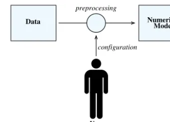
Operational usage. The model is run fully or partially unattended for producing regular outputs. Once configured, the simulation’s setup remains the same for an extended pe-riod of time. The emphasis is put on robustness and stability. We decided to tackle both scenarios with the same soft-ware package and ended up with the following goals (see Fig. 1):
– isolate the data reading routines from the rest of the model
– implement robust data handling with relevant error mes-sages for the end user
– allow the data model to be easily expanded (data model scalability)
– make it possible to easily change the data source (format and/or protocol) without any change in the model code itself
– preprocess the data on the fly
– implement a “best effort” approach with reasonable fall-back strategies in order to interrupt the simulation pro-cess only in the most severe cases
2 Architecture
Using the design philosophy guidelines laid out in Sect. 1.3 and in order to be able to reuse this software package in other models, we decided to implement this software package as a library named MeteoIO. We chose the C++ language in or-der to benefit from the object-oriented model as well as good performance and relatively easy interfacing with other pro-gramming languages. We also decided to invest a significant effort in documenting the software package both for the end users and for developers who would like to integrate it into their own models. More architectural principles are laid out in the sections below while the implementation details are given in Sects. 3 and 4.
2.1 Actors
The question of proper role assignment (Yu and Mylopoulos, 1994), or finding out who should decide, is central to the de-velopment of MeteoIO – carefully choosing whether the end user, the model relying on MeteoIO or MeteoIO itself is the appropriate actor to take a specific decision has been a re-curring question in the general design. For example, when temporally resampling data, the method should be chosen by the end user while the sampling rate is given by the numeri-cal model and the implementation details and error handling belong to MeteoIO.
2.2 Dependencies
When complex software packages grow, they often require more and more external dependencies (as third-party soft-ware libraries or third-party tools). When new features are added, it is natural to try to build on achievements of the community and not “reinvent the wheel”. However, this also has some drawbacks:
– These third-party components must be present on the end user’s computer.
– These components need to be properly located when compiling or installing the software package.
– These components have their own evolution, release schedule and platform support.
Therefore, as relying more on external components reduces the core development effort, it significantly increases the in-tegration effort. One must then carefully balance these two costs and choose the solution that will yield the least long-term effort.
Estimating that a complex integration issue represents a few days of work and a non-negligible maintenance effort, core MeteoIO features that were feasible to implement within a few days were redeveloped instead of integrating existing solutions. For the more peripheral features (like output plug-ins) we decided to rely on the most basic libraries at hand,
Numerical Model preprocessing
Data
configuration
User
Figure 1. Isolation of the data reading and preprocessing routines from the numerical model.
disregarding convenient wrappers which would introduce yet another dependency, and to give the user the possibility to de-cide which features to enable at compile time. Accordingly, MeteoIO requires no dependencies by default when it would have required more than 15 if no such mitigation strategy had been taken. A handful of dependencies can be activated when enabling all the optional features.
2.3 Manager/worker architecture
Many tasks have been implemented as a manager/worker ar-chitecture (see Fig. 2): a manager offers a high-level inter-face to the task (filtering, temporal interpolation, . . . ) while a worker implements the low-level, MeteoIO-agnostic core processing. The manager class implements the necessary fea-tures to efficiently convert MeteoIO-centric concepts and ob-jects to generic, low-level data ideal for processing. All of the heavily specialized programming concepts (object facto-ries, method pointers, etc) and their actual implementations are therefore hidden from both the high-level calls and the low-level processing. This architecture balances the needs of the casual developer using the library (relying on very sim-ple, high-level calls) as well as the casual developer expand-ing the library by contributexpand-ing some core processexpand-ing modules (data sources, data filters, etc).
Although this approach might seem inefficient (by adding extra steps in the data processing), it has contributed to the performance gains (as shown in Sect. 5.2) by making it pos-sible to rely on standard, optimized routines.
2.4 Flexibility
the user configure his simulation (Inishell, 2014). Moreover, instead of having to keep multiple files representing the data at various intermediate processing stages alongside a textual description of the processing steps that have been applied, it is possible to simply archive the raw data and the configura-tion file that then acts as a representaconfigura-tion of the preprocess-ing workflow. This greatly simplifies the data traceability for a given simulation.
For clarity, each step of the data reading, preprocessing and writing is described in its own section in the configura-tion file. There is no central repository or validaconfigura-tion of the keys to be found in this file, leaving each processing compo-nent free to manage its own configuration keys. On the other hand there is no global overview of which keys might have been provided by the user but will not be used by any com-ponent.
No assumptions are made about the sampling rate of the data read or the data required by the caller. It is assumed that the input data can be sampled at any rate, including irreg-ular sampling, and can be resampled to any timestamp, as requested by the caller. Moreover, any data field can be “no-data” at any time. This means that a given data set might con-tain for example precipitation sampled once a day, tempera-tures sampled twice an hour and snow height irregularly sam-pled. Practically, this prevents us from using standard sig-nal processing algorithms for resampling data, because these commonly assume a constant sampling rate and require that all timestamps have a value.
2.5 Modularity
A key to the long-term success of a software package is the modularity of its internal components. The choice of an object-oriented language (C++) has helped tremendously to build modular elements that are then combined to complete the task. The data storage classes are built on top of one another (through inheritance or by integrating one class as a member of another one) while the data path management is mostly built as a manager that links all the necessary compo-nents. A strong emphasis has been put on encapsulation by answering, for each new class, the following question: how should the caller interact with this object in an ideal world? Then the necessary implementation has been developed from this point of view, adding “non-ideal” bindings only when necessary for practical reasons.
2.6 Promoting interdisciplinary contributions
Modularity, by striving to define each data processing in a very generic way and by making each one independent of the others, presents external contributors with a far less intimidating context to contribute. The manager/worker ap-proach shown in Sect. 2.3 also facilitates keeping the mod-ules that are good candidates for third-party contributions simple and generic. Some templates providing a skeleton
between high and low level Complex, bridges the gap
Easy to expand, low level Easy to use, high level
expands... calls API...
User
Interface class
Worker class Manager class API
EXP
Figure 2. Manager/worker architecture; very often the interface and the manager are implemented in the same class, the interface being the public interface and the manager being the private implementa-tion.
of what should be implemented are also provided alongside documentation on how to practically contribute with a short list of points to follow for each kind of contribution (data plug-in, processing element, temporal or spatial interpola-tion).
2.7 Coding standards and methodology
The project started in late 2008 and is currently comprised of more than 52 000 lines, contributed by 12 contributors. 95 % of the code originates from the two main contributors. The code mostly follows the kernel coding style as well as the recommendations given by Rouson et al. (2011), giving the priority to code clarity. Literate programming is used with the doxygen tool (van Heesch, 2008).
Coding quality is enforced by requesting all committed code to pass the most stringent compiler warnings (all possi-ble warnings on gcc) including the compliance checks with recommended best practices for C++ (Meyers, 1992). The code currently compiles on Linux, Windows, OS X and An-droid.
The development methodology is mostly based on Ex-treme Programming (Beck and Andres, 2004) with short de-velopment cycles of limited scope, architectural flexibility and evolutions, frequent code reviews and daily integration testing. The daily integration testing has been implemented withctest (Martin and Hoffman, 2007), validating the core features of MeteoIO and recording the run time for each test. This shows performance regressions alongside feature regressions. Regular static analysis is performed using Cp-pcheck (Marjamäki, 2013) and less regularly with Flawfinder (Wheeler, 2013) to detect potential security flaws. Regu-lar leak checks and profiling is performed relying on the Valgrind instrumentation framework (Seward et al., 2013; Nethercote and Seward, 2007).
stan-dard iostream object. This object is then passed to the paral-lelization toolkit or library (such as MPI, the Message Pass-ing Interface) as a pure C structure through a very simple wrapper in the calling application.
3 Data structures
All data classes rely on the Standard Template Library (STL) (Musser et al., 2001) to a large extent that is available on all C++ compilers and may provide some low-level optimiza-tions while being quite high level. The design of the STL is also consistent and therefore a good model to follow: the data classes in MeteoIO follow the naming scheme and logic of the STL wherever possible, making them easier to use and remember by a developer who has some experience with the STL. They have been designed around the following specific requirements:
– offer high-level features for handling meteorological data and related data. Using them should make the call-ing code simpler.
– implement a standard and consistent interface. Their in-terface must be obvious to the caller.
– implement them in a robust and efficient way. Using them should make the calling code more robust and faster.
The range of high-level features has been defined accord-ing to the needs of models relyaccord-ing on MeteoIO as well as in terms of completeness. When appropriate and unambiguous the arithmetic operators and comparison operators have been implemented. Each internal design decision has been based on careful benchmarking.
Great care has been taken to ensure that the implemented functionality behaves as expected. Of specific concern is that corner cases (or even plain invalid calls) should never pro-duce a wrong result but strive to propro-duce the expected result or return an exception. A silent failure would lead to possibly erroneous results in the user application and must therefore be avoided at all cost.
3.1 Configuration
In order to automate the process of reading parameters from the end user configuration file, a specific class has been cre-ated to manage configuration parameters. The Config class stores the configuration options as a key-value couple of strings in a map. The key is built by prefixing the actual key with the section it belongs to. When calling a getter to read a parameter from the Config object, it converts data types on the fly through templates. It also offers several convenience methods, such as the possibility of requesting all keys match-ing a (simple) pattern or all values whose keys match a (sim-ple) pattern.
3.2 Dates
The Date class stores the GMT Julian day (including the time) alongside the time-zone information (because leap sec-onds are not supported, the reference is defined as being GMT instead of UTC). The Julian day is stored in double pre-cision which is enough for 1-second resolution while keeping dates arithmetic and comparison operators efficient. The con-version to and from split values is done according to Fliegel and van Flandern (1968). The conversion to and from various other time representations as well as various formatted time strings and rounding is implemented.
3.3 Geographic coordinates
The geographic coordinates are converted and stored as lati-tude, longitude and altitude in WGS84 by the Coords class. This allows an easy conversion to and from various Carte-sian geographic coordinates systems with a moderate loss of precision (of the order of 1 metre) that is still compatible with their use for meteorological data. Two different strate-gies have been implemented for dealing with the coordinate conversions:
– relying on a the proj4 third-party library (PROJ.4, 2013). This enables support of all coordinate systems but brings an external dependency.
– implementing the conversion to and from lati-tude/longitude. This does not bring any external depen-dency but requires some specific (although usually lim-ited) development.
Therefore the coordinate systems that are most commonly used by MeteoIO’s users have been reimplemented (currently the Swiss CH1903 coordinates, UTM and UPS; Hager et al., 1989) and seldom-used coordinate systems are supported by the third-party library. It is also possible to define a local coordinate system that uses a reference point as origin and computes easting and northing from this point using either the law of cosine or the Vincenty algorithm (Vincenty, 1977) for distance calculations. These algorithms are also part of the API and thus available to the developer.
3.4 Meteorological data sets
strategies have been implemented in order to merge measure-ments from close stations (for example when a set of instru-ments belongs to a given measuring network and another set, installed on the same mast, belongs to another network).
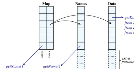
A static map does the mapping between predefined meteo-rological parameters (defined as an enum) and an index (see Fig. 3). A vector of strings stores a similar mapping between the predefined meteorological parameters’ names as strings and the same index (i.e. a vector of names). Finally a vec-tor of doubles (data vecvec-tor) svec-tores the actual data for each meteorological parameter, according to the index defined in the static map or names vector. When an extra parameter is added, a new entry is created in the names vector as well as a new entry in the data vector at the same index. The to-tal number of defined meteorological parameters is updated, making it possible to access a given meteorological field ei-ther by index (looping between zero and the total number of fields), by name (as string) or by predefined name (as enum). Methods to retrieve an index from a string or a string from an index (or enum) are also available.
3.5 Grids
Grids have been implemented for 1-D to 4-D data as tem-plates in the Array classes in order to accommodate different data types. They are based on the standard vector container and define the appropriate access by index (currently as row major order) as well as several helper methods (retrieving the minimum, maximum or mean value of the data contained in the grid, for example) and standard arithmetic operators be-tween grids and bebe-tween a grid and a scalar. A geolocalized version has been implemented in the GridObject classes that brings about added safety in the calling code by making it possible to check that two grids refer to the same domain before using them.
3.6 Digital elevation model
A special type of 2-D grid (based on the Grid2DObject class) has been designed to contain digital elevation model (DEM) data. This DEMObject class automatically com-putes the slope, azimuth and curvature as well as the sur-face normal vectors. It lets the developer choose between different algorithms: maximum downhill slope (Dunn and Hickey, 1998), four-neighbour algorithm (Fleming and Hof-fer, 1979) or two-triangle method (Corripio, 2003) with an eight-neighbour algorithm for border cells (Horn, 1981). The azimuth is always computed using Hodgson (1998). The two triangle method has been rewritten in order to be centred on the actual cell instead of node-centred, thus working with a local 3×3 grid centred around the pixel of interest instead of 2×2.The normals are also computed as well as the cur-vatures, using the method of Liston and Elder (2006).
The evaluation of the local slope relies on the eight imme-diate neighbours of the current cell. Because this offers only
extra parameters
Names Data
Map
index
enum
getName() from index
getData()
from enum getName()
from index, from name, from enum
Figure 3. Meteorological data set internal structure.
a limited number of meaningful combinations for comput-ing the slope, some more recent slope calculation algorithms that have been explored are actually exactly equivalent to the previously listed algorithms. In order to transparently han-dle the special cases represented by the borders (including cells bordering holes in the digital elevation model), a 3×3 grid is filled with the content of the cells surrounding the current cell. Cells that cannot be accessed (because they do not exist in the DEM) are replaced by nodata values. Then each slope algorithm works on this subgrid and implements workarounds if some required cells are set to nodata in order to be able to provide a value for each pixel that it received. This makes the handling of special cases very generic and computationally efficient.
Various useful methods for working with a DEM are also implemented, for example the possibility to compute the horizon of a grid cell or the terrain-following distance be-tween two points.
4 Components
4.1 Data flow overview
size_tgetMeteoData(
const Date& i_date,
std::vector<MeteoData>& vecMeteo );
Listing 1. MeteoIO call used by models to request all available me-teorological time series for a given time step.
boolgetMeteoData(
const Date& date,
const DEMObject& dem,
const MeteoData::Parameters& meteoparam,
Grid2DObject& result );
Listing 2. MeteoIO call used by models to request spatially inter-polated parameters for a given time step.
constraints specified by the user has been split into several steps (see Fig. 4):
1. getting the raw data
2. filtering and correcting the data
3. temporally interpolating (or resampling) the data if nec-essary
4. generating data from parameterizations if everything else failed
5. spatially interpolating the data if requested.
The practical steps are shown in Fig. 5. First, the raw data are read by the IOHandler component through a system of plug-ins. These plug-ins are low-level implementations pro-viding access to specific data sources and can easily be de-veloped by a casual developer. The data is read in bulk, be-tween two timestamps as defined by the BufferedIOHandler that implements a raw data buffer in order to prevent having to read data out of the data source for the next caller’s query. This buffer is then given for filtering and resampling to the MeteoProcessor. This will first filter (and correct) the whole buffer (by passing it to the ProcessingStack) since bench-marks have shown that processing the whole buffer at once is less costly than processing individually each of the time steps as they are requested. The MeteoProcessor then tempo-rally interpolates the data to the requested time step (if neces-sary) by calling the Meteo1DInterpolator. A last-resort stage is provided by the DataGenerator that attempts to generate the potentially missing data (if the data could not be tempo-rally interpolated) using parameterizations.
Finally, the data are either returned as such or spatially in-terpolated using the Meteo2DInterpolator. The whole pro-cess is transparently managed by the IOManager that re-mains the visible side of the library for requesting meteo-rological data. The IOManager offers a high-level interface
6692d179032205 b4116a96425a7f ecc2ef51af1740 959d3b6d07bce4 fa9f2af29814d9 82592e77a204a8
raw data Caller
Read Data
Filter Data
Resample Data
Generate Data
Spatialize Data
Figure 4. Simplified view of the MeteoIO dataflow.
as well as some configuration options, making it possible for example to skip some of the processing stages. The caller can nevertheless decide to manually call some of these compo-nents since they expose a developer-friendly, high-level API.
4.2 Data reading
All the necessary adaptations for reading data from a specific data source are handled by a specifically construed plug-in for the respective data source. The interface exposed by the plug-ins is very simple and their tasks very focused: they must be able to read the data for a specific time interval or a specific parameter (for gridded data) and fill the MeteoIO data structures, converting the units to the International Sys-tem of Units (SI). Similarly, they must be able to receive some MeteoIO data structures and write them out. Several helper functions and classes are available to simplify the pro-cess. This makes it possible for a casual developer to read-ily develop his own plug-in, supporting his own data source, with very little overhead.
In its current version MeteoIO includes plug-ins for read-ing and/or writread-ing time series and/or grids from Oracle and PostgreSQL databases, the Global Sensor Network (GSN) REST API (Michel et al., 2009), Cosmo XML (cos, 2013), GRIB, NetCDF, ARC ASCII, ARPS, GRASS, PGM, PNG, GEOtop, Snowpack and Alpine3D native file formats and a few others.
The proper plug-in for the user-configured data source is instantiated by the IOHandler that handles raw data read-ing. Usually, the IOHandler is itself called by the Buffere-dIOHandler in order to buffer the data for subsequent reads. The BufferedIOHandler is most often called with a single timestamp argument, computes an appropriate time interval and calls IOHandler with this time interval, filling its internal buffer.
4.3 Data processing
1 2
EXP
API API
API
API EXP
API
EXP EXP
EXP
read data; (from io.ini)
fill MeteoData and StationData convert units; read station list;
return data for
6692d179032205 b4116a96425a7f ecc2ef51af1740 959d3b6d07bce4 fa9f2af29814d9 82592e77a204a8
request 5000 data points >= 2010−07−10T08:32:00 request 5000 data points >= 2010−07−10T08:32:00
return vector of timestamp per station
in a vector of stations
get data chunk IOHandler BufferedIOHandler return data from buffer
BufferedIOHandler IOHandler
check if data in buffer load plugin if necessary
plugin
IOManager IOManager is data in buffer?
return data from buffer
fill filtered & interpolated buffers
MeteoProcessor DataGenerator
request data for 2010−07−11T08:32:00
2010−07−11T08:32
Caller raw data
Meteo1DInterpolator interpolate at timestamp or reaccumulate data buffer
ProcessingStack
ProcessingBlock filter data buffer
designed to be called by the user
designed to be expanded by the user end user configurable
ResamplingAlgorithms GeneratorAlgorithms
Figure 5. Meteorological data reading and processing workflow. The classes marked API are designed to be called by the user and the classes marked EXP are designed to be expanded by the user.
These two stages are handled by the ProcessingStack and the Meteo1DInterpolator, respectively.
The ProcessingStack reads the user-configured filters and processing elements and builds a stack of ProcessingBlock objects for each meteorological parameter and in the order declared by the end user. The time series are then passed to each individual ProcessingBlock, each block being one spe-cific filter or processing implementation. These have been di-vided into three categories:
– processing elements – filters
– filters with windowing.
The last two categories stem purely from implementation considerations: filtering a data point based on a whole data window yields different requirements than filtering a data point independently of the data series. Filters represent a form of processing where data points are either kept or re-jected. The processing elements on the other hand alter the value of one or more data points. Filters are used to detect and reject invalid data while processing elements are used to correct the data (for instance, correcting a precipitation input for undercatch or a temperature sensor for a lack of ventila-tion). These processing elements can also be used for sensi-tivity studies, by adding an offset or multiplying by a given factor.
As shown in Fig. 6, each meteorological parameter is as-sociated with a ProcessingStack object that contains a vector of ProcessingElement objects (generated through an object factory). Each ProcessingElement object implements a spe-cific data processing algorithm. The meteorological parame-ters mapping to their ProcessingStack is done in a standard map object.
4.3.1 Filters
Filters are used to detect and reject invalid data and therefore either keep or reject data points but don’t modify their value. Often an optional keyword “soft” has been defined that gives some flexibility to the filter. The following filters have been implemented:
– min, max, min_max. These filters reject out-of-range values or reset them to the closest bound if “soft” is de-fined.
– rate. This filters out data points if the rate of change is larger than a given value. Both a positive and a negative rate of change can be defined, for example for a different snow accumulation and snow ablation rate.
– standard deviation. All values outside ofyˆ±3σare re-moved.
– median absolute deviation. All values outside yˆ±
Pointer to Vector Map
string
parameter
ProcessingElement
call process() method
Pointer to ProcessingStack
Figure 6. Internal structure of the ProcessingStack.
– Tukey. Spike detection follows Goring and Nikora (2002).
– unheated rain gauge. This removes precipitation inputs that do not seem physical. The criterion that is used is that for precipitation to really occur, the air and surface temperatures must be at most 3◦C apart and relative hu-midity must be greater than 50 %. This filter is used to remove invalid measurements from snow melting in an unheated rain gauge after a snow storm.
4.3.2 Processing elements
Processing elements represent processing that alters the value of one or more data points, usually to correct the data. The following processing elements have been implemented: – Mean, median or wind average average over a user-specified period. The period is defined as a minimum duration and a minimum number of points. The window centring can be specified, either left, centre or right. The wind averaging performs the averaging on the wind vec-tor.
– Exponential or weighted moving average smooths the data either with an exponential or weighted moving av-erage (EMA, WMA respectively) smoothing algorithm.
– Two poles, low-pass Butterworth is according to Butter-worth (1930).
– Add, mult, and suppr make it possible to add an offset or multiply by a given factor (constant or either hourly, daily or monthly and provided in a file), for sensitiv-ity studies or climate change scenarios or totally delete a given meteorological parameter.
– Unventilated temperature sensor correction corrects a temperature measurement for the radiative heating on an unventilated sensor, according to Nakamura and Mahrt (2005) or Huwald et al. (2009).
– Undercatch. Several corrections are offered for precip-itation undercatch, either following Hamon (1972) and Førland et al. (1996) or following the WMO corrections (Goodison et al., 1997). Overall, the correction coef-ficients for 15 different rain gauges have been imple-mented. Since the WMO corrections were not available for shielded Hellmann rain gauges, a fit has been com-puted based on published data (Wagner, 2009; Daqing et al., 1999). The correction for the Japanese RT-3 rain gauges has been implemented following Yokoyama et al. (2003). It is also possible to specify fixed correc-tion coefficients for snow and mixed precipitacorrec-tion. – precipitation distribution. The precipitation sum can be
distributed over preceding time steps. This is useful for example when daily sums of precipitation are written at the end of the day in an otherwise hourly data set. The data window can also be configured by the end user: by default the data are centred around the requested data point. But it is also possible to force the data window to be left or right centred. An extra option “soft” allows the data window to be centred as specified by the end user if applica-ble or to shift the window according to a “best effort” strategy if the data do not permit the requested centring.
4.4 Resampling
If the timestamp requested by the caller is not present in the data (either it has been filtered out or it was not present from the beginning), temporal interpolations will be performed. The Meteo1DInterpolator is responsible for calling a tempo-ral interpolation method for each meteorological parameter as configured by the end user. The end user chooses between the following methods of temporal interpolation for each me-teorological parameter separately:
– no interpolation. If data exist for the requested times-tamp they will be returned or remain nodata otherwise. – nearest neighbour. The closest data point in the raw data
that is not nodata is returned.
– linear. The value is linearly interpolated between the two closest data points.
– accumulation. The raw data are accumulated over the period provided as argument.
– daily solar sum. The potential solar radiation is gener-ated as to match the daily sum as provided in the input data.
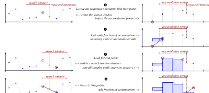
1
2
3
4
Add fraction of accumulation −> <− linearly interpolate
sum all samples until (insertion_index−1) −> <− within a search window distance
Look for end point: assuming a linear accumulation rate Calculate fraction of accumulation −>
before the accumulation period −> <− within the search window
Locate the requested timestamp, find start point:
0000000 0000000 0000000 0000000 0000000 1111111 1111111 1111111 1111111 1111111 000000 000000 000000 000000 000000 000000 000000 000000 000000 000000 000000 000000 000000 000000 000000 111111 111111 111111 111111 111111 111111 111111 111111 111111 111111 111111 111111 111111 111111 111111 0000000 0000000 0000000 0000000 0000000 1111111 1111111 1111111 1111111 1111111 000000 000000 000000 000000 000000 000000 000000 000000 000000 000000 000000 000000 000000 000000 111111 111111 111111 111111 111111 111111 111111 111111 111111 111111 111111 111111 111111 111111 000000 000000 000000 000000 000000 000000 000000 000000 000000 000000 000000 000000 000000 000000 111111 111111 111111 111111 111111 111111 111111 111111 111111 111111 111111 111111 111111 111111 000000 000000 000000 000000 000000 000000 000000 000000 000000 000000 000000 000000 000000 000000 000000 000000 111111 111111 111111 111111 111111 111111 111111 111111 111111 111111 111111 111111 111111 111111 111111 111111 0000000 0000000 0000000 0000000 0000000 1111111 1111111 1111111 1111111 1111111 000000 000000 000000 000000 111111 111111 111111 111111 search window search window search window
requested timestamp accumulation periodrequested timestamp
accumulation period
accumulation period
accumulation period
Figure 7. Resampling and reaccumulation operations.
variable sampling rate for both the input and output data prevents the utilization of well-known signal analysis algo-rithms. Moreover, some meteorological parameters require a specific processing, such as precipitation that must be ac-cumulated over a given period. The following approach has therefore been implemented (see in Fig. 7): for each re-quested data point, if the exact timestamp cannot be found or in the case of reaccumulation, the index where the new point should be inserted will be sought first. Then the pre-vious valid point is sought within a user-configured search distance. The next valid point is then sought within the user-configured search distance from the first point. Then the re-sampling strategy (nearest neighbour, linear or reaccumula-tion) uses these points to generate the resampled value. Other resampling algorithms may be implemented by the user that would use more data points.
When no previous or next point can be found, the resam-pling extrapolates the requested value by looking at more valid data points respectively before or after the previously found valid points. Because of the significantly increased risk of generating a grossly out of bound value, this behaviour must be explicitly enabled by the end user.
4.5 Data generators
In order to be able to return a value for a given timestamp there must be enough data available in the original data source. These data have to pass the filters set up by the end user and may then be used for resampling. In the case that data are absent or filtered out there is still a stage of last re-sort: the data can be generated by a parameterization relying on other parameters. The end user configures a list of algo-rithms for each meteorological parameter. These algoalgo-rithms are implemented as classes inheriting from the GeneratorAl-gorithms. The DataGenerator class acts as their high-level interface. The algorithms range from very basic, such as as-signing a constant value, to quite elaborate. For instance the measured incoming solar radiation is compared to the
poten-tial solar radiation resulting in a solar index. The solar index is used in a parameterization to compute a cloud cover that is given to another parameterization to compute a long-wave radiation.
The GeneratorAlgorithms receive a set of meteorological parameters for one point and one timestamp. The DataGen-erator walks through the user-configured list of genDataGen-erators, in the order of their declaration by the end user, until a valid value can be returned. The returned value is inserted into the data set and either returned to the caller or used for spatial interpolations.
The following generators have been implemented: – standard pressure generates a standard pressure that
only depends on the elevation.
– constant generates a constant value as provided by the user.
– sinusoidal generates a value with sinusoidal variation, either on a daily or a yearly period. The minimum and maximum values are given as arguments as well as the position of the first minimum.
– relative humidity generates a relative humidity value from either dew point temperature or specific humidity. – clearsky_lw generates a clear sky incoming long-wave radiation, choosing between several parameterizations (Brutsaert, 1975; Dilley and O’brien, 1998; Prata, 1996; Clark and Allen, 1978; Tang et al., 2004; Idso, 1981). – allsky_lw generates an incoming long-wave radiation
measured snow heights greater than 10 cm and a grass albedo of 0.23 otherwise. If no measured snow height is available, a constant 0.5 albedo will be assumed. It is possible to chose between several parameterizations (Unsworth and Monteith, 1975; Omstedt, 1990; Craw-ford and Duchon, 1999; Konzelmann et al., 1994).
– potential radiation generates an incoming short-wave radiation (or reflected short-wave radiation) from a mea-sured long-wave radiation using a reciprocal Unsworth generator.
4.6 Spatial interpolations
If the caller requests spatial grids filled with a specific pa-rameter, two cases may arise: either the data plug-in reads the data as grids and can directly return the proper grid or it reads the data as point measurements. In this case, the data must be spatially interpolated. The end user configures a list of potential algorithms and sets the respective arguments to use for each meteorological parameter.
The Meteo2DInterpolator reads the user configuration and evaluates for each parameter and at each time step which algorithm should be used for the current time step, using a simple heuristic provided by the interpolation algorithm itself. Of course, relying on simple heuristics for determin-ing which algorithm should be used does not guarantee that the best result will be attained but should nonetheless suf-fice most of the time. This implies a trade-off between ac-curacy (selecting the absolutely best method) and efficiency (not spending too much time selecting a method that most probably is the one determined by the heuristic). The objec-tive is to ensure robust execution despite the vast diversity of conditions. The number of available data points often emi-nently influences the applicability of a given algorithm and without the flexibility to define fall-back algorithms frequent disruptions of the process in an operational scenario might ensue.
Most spatial interpolations are performed using a trend/residuals approach: the point measurements are first detrended in elevation, then the residuals are spatially interpolated and for each pixel of the resulting grid the elevation trend back is applied. Of course, the user can specify an algorithm that does not include detrending.
The following spatial interpolations have been imple-mented:
– filling the domain with a constant value (using the aver-age of all stations)
– filling the domain with a constant value with a lapse rate (assuming the average value occurs at the average of the elevations)
– filling the domain with a standard pressure that only de-pends on the elevation at each cell
– spatially interpolating the dew point temperature before converting it back to a relative humidity at each cell as in Liston and Elder (2006)
– spatially interpolating the atmospheric emissivity be-fore converting it back to an incoming long-wave ra-diation at each cell
– inverse distance weighting (IDW) with or without a lapse rate
– spatially interpolating the wind speed and correcting it at each point depending on the local curvature as in Ryan (1977)
– spatially interpolating the wind speed and correcting it at each point depending on the local curvature as in Lis-ton and Elder (2006)
– spatially interpolating the precipitation, then pushing the precipitation down the steep slopes as in Spence and Bavay (2013)
– ordinary kriging with or without a lapse rate as in Goovaerts (1997) with variogram models as in Cressie (1992)
– spatially interpolating the precipitation and correcting it at each point depending on the topographic wind expo-sure as in Winstral et al. (2002)
– loading user-supplied grids
– finally, it is also possible to activate a “pass-through” method that simply returns a grid filled with nodata. Relying on the fall-back mechanism described above it is, for example, possible to configure the spatial interpolations to read user-supplied grids for some specific time steps, re-verting to ordinary kriging with a lapse rate if enough stations can provide data and no user-supplied grids are available for this time step, reverting to filling the grid with the measure-ments from a single station with a standardized lapse rate if nothing else can be done. Everything happens transparently from the point of view of the caller.
Lapse rates
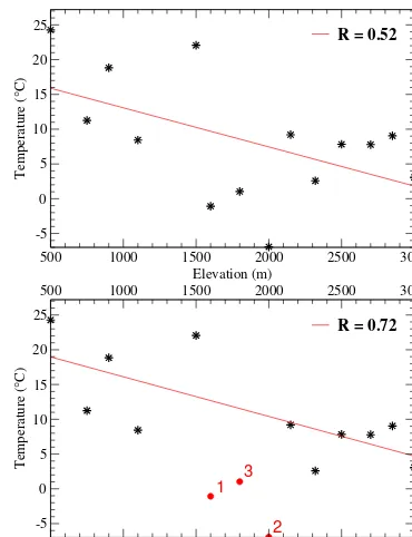
1. The lapse rate is computed.
2. If the lapse rate’s correlation coefficient is better than a 0.7 threshold, the determined lapse rate will be used as such.
3. If this is not the case, the point that degrades the cor-relation coefficient the most will be sought: for each point, the correlation coefficient is computed without this point. The point whose exclusion leads to the high-est correlation coefficient is suppressed from the data set for this meteorological parameter and at this time step. 4. If the correlation coefficient after excluding the point
determined at 3 is better than the 0.7 threshold, the de-termined lapse rate will be used as such, otherwise the process will loop back to point 3.
The process runs until at most 15 % of the original data set points have been suppressed or when the total number of points falls to four, in order to keep a reasonable number of points in the data set. This is illustrated in Fig. 8: the initial set of points has a correlation coefficient that is lower than the threshold, leading to the removal of the three points in the right-hand side panel, resulting in a coefficient above the threshold.
Finally, most of the spatial interpolations algorithms offer their own fall-back for the lapse rate: it is often possible to manually specify a lapse rate to be used when the data-driven lapse rate has a correlation coefficient that remains less than the 0.7 threshold.
4.7 Grid rescaling
Rescaling gridded meteorological data to a different resolu-tion is often necessary for reading a grid (and bringing it in line with the DEM grid) or for writing a grid out (for exam-ple, as a graphical output). Since meteorological parameters at the newly created grid points mostly depend on their im-mediate neighbours and in order to keep the computational costs low, standard image processing techniques have been used: the rescaling can either be done by applying the nearest neighbour, bi-linear or cubic B-spline algorithms. These al-gorithms are very efficient and appropriate for rescaling grids to a higher resolution without any matching DEM since no gradient correction will be performed.
4.8 Miscellaneous utilities
In order to provide common algorithms to the various com-ponents, several classes have been designed that ment well-known algorithms. These classes have been imple-mented in quite a generic way, striving for readability, stabil-ity – no surprising behaviour – and acceptable performance. A basic set of monodimensional statistical algorithms have been implemented as they are often required by the filters or the spatial interpolation methods. These are completed by
500 1000 1500 2000 2500 3000
Elevation (m) -5
0 5 10 15 20 25
Temperature (°C)
R = 0.52
1
2 3
500 1000 1500 2000 2500 3000
-5 0 5 10 15 20 25
Temperature (°C)
R = 0.72
Figure 8. Removing outliers for computing lapse rates.
a least-square regression solver that can be used on any statis-tical model by inheriting from a base class and implementing the model itself. This required a basic set of arithmetic ma-trix operations, also required for kriging. The Mama-trix class strives to remain as close as possible to the standard math-ematical notation and implements all the basic operations: addition, subtraction, multiplication, determinant, transpo-sition. The generic inversion is implemented by first per-forming the LU factorization (using the Doolittle algorithm; Duff et al., 1986) and then backward and forward solving of LU×A−1=I (Press et al., 1992). This represents a good balance between complexity and efficiency since more ad-vanced methods provide benefits only for very large matri-ces. For the case of tridiagonal matrices, the Thomas algo-rithm is offered (Thomas, 1949).
In order to isolate platform-specific code, several classes and functions have been implemented: functions dealing with file and path handling, such as checking whether a file name is valid, whether a file exists, the copying of files, extracting a path or an extension and microsecond-resolution timers. The timers are offered for benchmarking purposes with a res-olution of up to 1 ns with very low overhead.
4.9 Optimizations
In order to optimize the algorithms based on distances, such as inverse distance weighting, it has been necessary to op-timize the computation of expressions such as 1/√x. This has been achieved through a fast inverse square root approxi-mation implementation (Lomont, 2003) that has been shown to give at most 1.7 % relative error and deliver at least a 4-times speed-up. Similarly, a method for fast computation of cubic roots has been implemented based on a single itera-tion Halley’s method with a bit hack approximaitera-tion provid-ing the seed (Lancaster, 1942) and a fast computation of powers based on bit hacks and exponentiation by squaring (Montgomery, 1987). These are grouped in a specific names-pace and header file alongside other numerical optimizations (Hastings et al., 1955).
5 Benchmarks
Several numerical models developed by different institutions rely on MeteoIO for their I/O needs. Several specialized ap-plications (mostly web services) have also been developed in different countries based on MeteoIO. It is also used regularly for several warning systems and research projects around the world. Such applications include the Common Information Platform for Natural Hazards GIN (gin, 2014), sensorscope (Barrenetxea et al., 2008), the GeoTop model (Endrizzi et al., 2014), the Hydrosys project (Kruijff et al., 2010) or the avalanche warning services in Switzerland, Canada, India or Austria.
In order to check the design goals against real-world ap-plications, some benchmarks are presented in this section. These have been conducted on a recent octo-core computer powered by a 64 bits Intel Core i7 processor (3612QM) equipped with 8 GB of RAM. The processor runs between 1.2 and 3.1 GHz and reaches a CPU Mark of 6834 (http:// www.cpubenchmark.net/). The benchmarks have been com-piled by the GNU Compiler Collection (GCC) version 4.7.2 both for C++, C and Fortran.
5.1 Ease of extension
In order to check whether it is really easy for third parties to contribute to MeteoIO, a test was set up asking participants to develop a basic filter. The filter that had to be developed is a simple filter on the incoming long-wave radiation, rejecting all data outsideminσ T4andmaxσ T4.
Once their system was properly configured (and checked by running a simple test), the participants were provided with a sheet with instructions and questions and asked to imple-ment the required filter following the official docuimple-mentation, working alone and without assistance. Ten participants took the test, including eight PhD students. The participants use computers for their daily work (mostly using Matlab or R) with only four participants having a previous experience in C
or C++. In order to better discriminate between the overhead (i.e. integrating one’s development within MeteoIO) and the intrinsic complexity of the required processing (i.e. the logic of the filter that had to be implemented), the participants were asked to first write an empty filter and then to implement the logic of the filter.
The results show that for an average user (the median of the results), writing, compiling and testing an empty filter re-quires 40 min while implementing and testing the real filter requires 50 min. Since only a limited number of users did par-ticipate in this test, this tends to show a worst-case scenario by being overly sensitive to specific issues: one user spent quite a lot of time trying to make his test work, only to re-alize that he was not testing with his latest changes, another one used a wrong test data set, etc. Based on the response of the test users themselves, the initial programming abili-ties were not really a major factor in their achievements but mostly the ability to follow the step-by-step instructions.
5.2 Meteorological data processing benchmarks Reading meteorological data stored in an ASCII file bears a significant overhead. The file needs to be read line by line, each line needs to be split up based on a predefined delim-iter, the values need to be converted from strings to their re-spective data types and the data need to be stored in mem-ory for further processing. A comparative illustration of dif-ferent programming environments and their performance in completing the aforementioned task for a 873 kB file contain-ing hourly data for one station and 1 year is given in Fig. 9. The GNU compilers gcc, g++ and gfortran were used to ob-tain the benchmark executables. Clearly C++ and MeteoIO, which is programmed in C++ and utilizes the GNU STL and streams implementations, show the same performance. The efficient dynamic memory management gives C the over-all advantage, whereas Fortran95 (static) shows good per-formance for parsing values to doubles, with the drawback that the exact layout and size of the file need to be known at compile time. Allowing these properties to be dynamic, slows down the performance. Apart from only reading the data, MeteoIO performs a unit conversion and finally stores the data in MeteoData objects which are then used for further processing and exposed to the user.
D
ur
at
io
n
(m
ill
is
ec
on
ds
)
0 20 40 60 80
Programming Environment
MeteoIO (STL) F95 (dynamic) C++ (STL) F95 (static) C (malloc)
I/O, line split, parsing, storage Unit conversion
copying to MeteoData, post processing
Figure 9. Performance when reading a SMET ASCII file with 1 year of hourly data into memory.
D
u
ra
ti
on
(
se
co
n
d
s)
0 20 40 60 300 400 500 600
MeteoIO Version
2.0.1 2.1.1 2.1.2 2.1.3 2.3.0 2.3.1 2.4.0 2.4.1 2.4.2
File I/O Filtering Resampling Other Mar '11
Nov '12 May '12
Dec '13 Feb '14 Sep '11
Oct '11
Mar '13
Jul '14
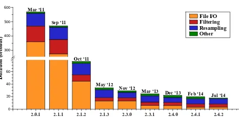
Figure 10. Performance increase in MeteoIO (March 2011 until February 2014).
moment in time. Since MeteoData objects are copied and instantiated during all processing steps focusing on the formance of the copy constructor yielded a spectacular per-formance boost. Further improvements leading up to version 2.1.3 are mainly comprised of an efficient use of file pointers regarding I/O and a redesign of the processing capabilities, namely reducing the amount of copies necessary when deal-ing with series of data points durdeal-ing filterdeal-ing and resampldeal-ing. Optimizations in all parts of the code bring about a constant improvement of the MeteoIO performance albeit a significant increase of features and requirements. The strategy through-out development is to write correct code following best prac-tice design rules, to then profile it using static and dynamic analysis tools as laid out in Sect. 2.7 and to optimize where significant improvements can be expected based on the re-sults of the profiling.
5.3 Spatial interpolations benchmarks
Unsurprisingly, most of the spatial interpolation algorithms scale asO(n). However, since there is some overhead (con-structing the required spatial interpolator, setting the grid metadata, gathering the necessary data) it is interesting to see how the real-world scalability is. To this effect, the “pass-through” interpolation has been used that fills the grid with nodata by calling the optimized STL methods on the
underly-1 10 100 1 k 10 k 100 k 1 M 10 M
Number of cells 0.0001
0.001 0.01 0.1 1 10 100
Time (s)
1*1 10*10 100*100 1k*1k
grid size
None Cst Cst_lapse Idw Idw_lapse ODKrig_lapse
Figure 11. Benchmarks of some spatial interpolation algorithms for various grid sizes for 7 input stations (plain lines) and 14 input sta-tions (dotted lines).
ing data container. Different spatial interpolations have been benchmarked for different grid sizes, ranging from one cell to 25 million cells. Two scenarios have been used: one pro-viding 7 meteorological stations as input and one propro-viding 14 meteorological stations as input, each station providing 2 months of hourly data in a 130 kb file.
The results are shown in Fig. 11. The linear behaviour starts to be visible after around 0.3 ms which would then be the total overhead for spatial interpolations. This overhead also depends on the chosen algorithm: for example the sim-ple pass-through has a very low 0.1 ms overhead (there is nothing to prepare before filling the grid) to 0.4 ms for ordi-nary kriging with 14 stations (the necessary matrices have to be computed with the station data before filling the grid).
One year,
start of file One year,end of file
Fourteen years 24 spatial
interpolations
0.1 1 10
time (s)
15 stations One station 7 stations
Figure 12. Benchmarks of different usage scenarios: reading one year of hourly data from the beginning of a large file, reading one year of hourly data at the end of a large file, reading fourteen years of hourly data, spatially interpolating seven meteorological param-eters every hour for a day. These scenarios are repeated for one sta-tion and fifteen stasta-tions.
(visible for small grids that exhibit a non-linear behaviour depending on the number of stations) and another 10-times slowdown compared to IDW_LAPSE.
5.4 Usage scenarios benchmarks
Although the MeteoIO library offers various components of interest to numerical models, its primary usage is to read, preprocess and potentially spatially interpolate meteorologi-cal data. Therefore, a benchmark has been set up with various scenarios, all based on fifteen stations providing hourly data for fourteen years (representing 14 Mb on average). The data is read from files, all parameters are checked for min/max, the precipitation is corrected for undercatch, the snow height is filtered for its rate of change, then all parameters are lin-early interpolated if necessary while the precipitation is reac-cumulated. The spatial interpolations rely on IDW for some parameters, WINSTRAL for the precipitation and LISTON for the wind direction. The following scenarios have been defined: reading the hourly data necessary to simulate one season either at the beginning of the file or at the end, reading the hourly data required to simulate the full period contained in the files and reading and spatially interpolating hourly data once per hour for a day over a 6500 cells DEM.
These scenarios have been further split in two: only one station providing the data or fifteen stations providing the data. For the spatial interpolations, since it made little sense to benchmark very specific algorithms able to handle only one station, then seven and fifteen stations have been used.
The results are presented in Fig. 12. First, this shows that when the data are extracted as time series, the preprocess-ing time is negligible compared to what would be a realis-tic model run time. Working on raw data and preprocessing the data on the fly thus does not introduce any performance penalty. Then the run time scales linearly both with the num-ber of stations and with the total duration, although the
posi-tion of the data in the file has a direct impact on the perfor-mances. For the case of the spatial interpolations, the scaling is still linear with the number of stations but the performance impact is much higher; however this should still remain much lower than most models’ time step duration.
6 Conclusions
In order to split the data preprocessing and data consumption tasks in numerical models, the MeteoIO library has been de-veloped. This has allowed the numerical models to focus on their core features and to remove a lot of data preprocessing code as well as to peek into the data that are sent to the core numerical routines. This has also led to fruitful developments in the preprocessing stage much beyond what was originally performed on the numerical models. A careful design made it possible for casual users to easily contribute to data filters or parameterizations. This ease of contribution to MeteoIO make it a great test bed for new preprocessing methods with a direct link to actual numerical models. A contributor with little or no previous C++ experience can contribute simple algorithms with a relatively minor time investment. In terms of performance, continuous benchmarking and profiling have led to major improvements and keep the preprocessing com-putational costs well balanced compared to the data acquisi-tion costs.
Today, the MeteoIO library offers great flexibility, reliabil-ity and performance and has been adopted by several models for their I/O needs. These models have all benefited from the shared developments in MeteoIO and as such offer an in-creased range of application and an inin-creased robustness in regard to their forcing data.
Code availability
The MeteoIO library is available under the GNU Lesser General Public License v3.0 (LGPL v3) on http://models. slf.ch/p/meteoio/ both as source code (from the source ver-sion control system or as packages) or as precompiled bina-ries for various platforms. Stable releases are announced on http://freecode.com/projects/meteoio.
The documentation must be generated from the source code or is available as html in the precompiled packages. The documentation for the last stable release is available online at http://models.slf.ch/docserver/meteoio/html/index.html. De-tailed installation instructions are available at http://models. slf.ch/p/meteoio/page/Getting-started/.
INFSO) on spatial analysis tools for on-site environmental moni-toring and management and the Swiss National Science Foundation and AAA/SWITCH-funded Swiss Multi Science Computing Grid project (http://www.smscg.ch).
The authors would like to thank M. Lehning and C. Fierz for their support as well as N. Wever, L. Winkler, M. Mbengue, C. Perot, D. Zanella, M. Diebold, C. Groot, T. Schumann and R. Spence for their contribution to MeteoIO. The authors would also like to thank all the colleagues who contributed their time for performing the extension test! The authors are also grateful to the anonymous reviewers who contributed to improve the quality of this paper.
Edited by: A. Sandu
References
Ballou, D. P. and Pazer, H. L.: Modeling data and process quality in multi-input, multi-output information systems, Manage. Sci., 31, 150–162, 1985.
Barrenetxea, G., Ingelrest, F., Schaefer, G., Vetterli, M., Couach, O., and Parlange, M.: Sensorscope: Out-of-the-box environmen-tal monitoring, In Information Processing in Sensor Networks, 2008, IPSN’08, International Conference, 332–343, IEEE, 2008. Beck, K. and Andres, C.: Extreme Programming Explained:
Em-brace Change, Addison-Wesley Professional, 2nd Edn., 2004. Brutsaert, W.: On a derivable formula for long-wave radiation from
clear skies, Water Resour. Res., 11, 742–744, 1975.
Butterworth, S.: On the theory of filters amplifiers, Experimental Wireless & the Wireless Engineer, 7, 536–541, 1930.
Clark, G. and Allen, C.: The estimation of atmospheric radiation for clear and cloudy skies, in: Proc. 2nd National Passive Solar Conference (AS/ISES), 675–678, 1978.
Corripio, J. G.: Vectorial algebra algorithms for calculating terrain parameters from DEMs and solar radiation modelling in moun-tainous terrain, Int. J. Geogr. Inf. Sci., 17, 1–23, 2003.
Consortium for Small-scale Modeling: available at: http://www. cosmo-model.org/ (last access: 30 May 2014), 2013.
Crawford, T. M. and Duchon, C. E.: An improved parameterization for estimating effective atmospheric emissivity for use in calcu-lating daytime downwelling longwave radiation, J. Appl. Meteo-rol., 38, 474–480, 1999.
Cressie, N.: Statistics for spatial data, Terra Nova, 4, 613–617, 1992. Daqing, Y., Esko, E., Asko, T., Ari, A., Barry, G., Thilo, G., Boris, S., Henning, M., and Janja, M.: Wind-induced precipi-tation undercatch of the Hellmann gauges, Nord. Hydrol., 30, 57–80, 1999.
Dilley, A. and O’brien, D.: Estimating downward clear sky long-wave irradiance at the surface from screen temperature and pre-cipitable water, Q. J. Roy. Meteor. Soc., 124, 1391–1401, 1998. Duff, I. S., Erisman, A. M., and Reid, J. K.: Direct Methods for
Sparse Matrices, Clarendon Press, Oxford, 1986.
Dunn, M. and Hickey, R.: The effect of slope algorithms on slope estimates within a GIS, Cartography, 27, 9–15, 1998.
Durand, Y., Brun, E., Merindol, L., Guyomarc’h, G., Lesaffre, B., Martin, E.: A meteorological estimation of relevant parameters for snow models, Ann. Glaciol., 18, 65–71, 1993.
Endrizzi, S., Gruber, S., Dall’Amico, M., and Rigon, R.: GEOtop 2.0: simulating the combined energy and water balance at and below the land surface accounting for soil freezing, snow cover and terrain effects, Geosci. Model Dev., 7, 2831–2857, doi:10.5194/gmd-7-2831-2014, 2014.
Fleming, M. D. and Hoffer, R. M.: Machine processing of landsat MSS data and DMA topographic data for forest cover type map-ping, Tech. Rep. LARS Technical Report 062879, Laboratory for Applications of Remote Sensing, Purdue University, 1979. Fliegel, H. F. and van Flandern, T. C.: Letters to the editor: a
ma-chine algorithm for processing calendar dates, Commun. ACM, 11, 657, doi:10.1145/364096.364097, 1968.
Førland, E. J., Allerup, P., Dahlstrøm, B., Elomaa, E., Jonsson, T., Madsen, H., Per, J., Rissanen, P., Vedin, H., and Vejen, F.: Man-ual for Operational Correction of Nordic Precipitation Data, DNMI-Reports 24/96 KLIMA, 1996.
gin: Common Information Platform for Natural Hazards, available at: http://www.gin-info.admin.ch/ (last access: 20 October 2014), 2014.
Goodison, B., Louie, P., and Yang, D.: The WMO solid pre-cipitation measurement intercomparison, World Meteorological Organization-Publications-WMO TD, 65–70, 1997.
Goovaerts, P.: Geostatistics for Natural Resources Evaluation, Ox-ford University Press, 1997.
Goring, D. G. and Nikora, V. I.: Despiking acoustic Doppler ve-locimeter data, J. Hydraul. Eng., 128, 117–126, 2002.
Hager, J. W., Behensky, J. F., and Drew, B. W.: The Universal Grids: Universal Transverse Mercator (UTM) and Universal Po-lar Stereographic (UPS), Edition 1, Tech. rep., Defense Mapping Agency, 1989.
Hamon, W. R.: Computing actual precipitation, in: Distribution of precipitation in mountaineous areas, Geilo symposium 1, 159– 174, World Meteorological Organization, 1972.
Hastings, C., Hayward, J. T., and Wong, J. P.: Approximations for digital computers, Vol. 170, Princeton University Press, Prince-ton, NJ, 1955.
Hodgson, M. E.: Comparison of angles from surface slope/aspect algorithms, Cartogr. Geogr. Inform., 25, 173–185, 1998. Horn, B. K.: Hill shading and the reflectance map, Proc. IEEE, 69,
14–47, 1981.
Huwald, H., Higgins, C. W., Boldi, M.-O., Bou-Zeid, E., Lehn-ing, M., and Parlange, M. B.: Albedo effect on radiative errors in air temperature measurements, Water Resour. Res., 45, W08431, doi:10.1029/2008WR007600, 2009.
Idso, S.: A set of equations for full spectrum and 8-to 14-µm and 10.5-to 12.5-µm thermal radiation from cloudless skies, Water resources research, 17, 295–304, 1981.
Inishell: A flexible configuration interface for numerical models: available at: https://models.slf.ch/p/inishell/ (last access: 30 Oc-tober 2014), 2014.
Iqbal, M.: An Introduction to Solar Radiation, Academic Press, 1983.