https://doi.org/10.5194/gmd-10-4129-2017 © Author(s) 2017. This work is distributed under the Creative Commons Attribution 3.0 License.
Improved method for linear carbon monoxide simulation and
source attribution in atmospheric chemistry models
illustrated using GEOS-Chem v9
Jenny A. Fisher1,2, Lee T. Murray3, Dylan B. A. Jones4,5, and Nicholas M. Deutscher1
1Centre for Atmospheric Chemistry, School of Chemistry, University of Wollongong, Wollongong, NSW, Australia 2School of Earth and Environmental Sciences, University of Wollongong, Wollongong, NSW, Australia
3Department of Earth and Environmental Sciences, University of Rochester, Rochester, NY, USA 4Department of Physics, University of Toronto, Toronto, ON, Canada
5Joint Institute for Regional Earth System Science and Engineering, University of California, Los Angeles, CA, USA
Correspondence to:Jenny A. Fisher ([email protected]) Received: 7 April 2017 – Discussion started: 3 May 2017
Revised: 19 September 2017 – Accepted: 27 September 2017 – Published: 15 November 2017
Abstract.Carbon monoxide (CO) simulation in atmospheric chemistry models is frequently used for source–receptor analysis, emission inversion, interpretation of observations, and chemical forecasting due to its computational efficiency and ability to quantitatively link simulated CO burdens to sources. While several methods exist for modeling CO source attribution, most are inappropriate for regions where the CO budget is dominated by secondary production rather than direct emissions. Here, we introduce a major update to the linear CO-only capability in the GEOS-Chem chem-ical transport model that for the first time allows source– region tagging of secondary CO produced from oxidation of non-methane volatile organic compounds. Our updates also remove fundamental inconsistencies between the CO-only simulation and the standard full chemistry simulation by us-ing consistent CO production rates in both. We find that rela-tive to the standard chemistry simulation, CO in the original CO-only simulation was overestimated by more than 100 ppb in the model surface layer and underestimated in outflow re-gions. The improved CO-only simulation largely resolves these discrepancies by improving both the magnitude and location of secondary production. Despite large differences between the original and improved simulations, however, model evaluation with the global dataset used to benchmark GEOS-Chem shows negligible change to the model’s abil-ity to match the observations. This suggests that the
cur-rent GEOS-Chem benchmark is not well suited to evaluate model changes in regions influenced by biogenic emissions and chemistry, and expanding the dataset to include obser-vations from biogenic source regions (including those from recent aircraft campaigns) should be a priority for the GEOS-Chem community. Using Australasia as a case study, we show that the new ability to geographically tag secondary CO production provides significant added value for interpreting observations and model results in regions where primary CO emissions are low. Secondary production dominates the CO budget across much of the world, especially in the Southern Hemisphere, and we recommend future model–observation and multi-model comparisons implement this capability to provide a more complete understanding of CO sources and their variability.
1 Introduction
in chemical transport models (CTMs) and chemistry–climate models (CCMs), as its only chemical loss is through reac-tion with OH. As long as the OH distribureac-tion and chemical sources are known (i.e., extracted from a full chemical sim-ulation) or can be parameterized, then the concentration of CO can be recalculated with an ordinary differential equa-tion that is linear in the CO concentraequa-tion and not coupled to other time-varying species. This linear CO simulation is highly computationally efficient, avoiding the need to solve the stiff chemical equations that dominate resource use in CTMs and CCMs (Duncan et al., 2007). Emitted CO can also easily be “tagged” by source region or type and followed as it is transported to receptor regions downwind, providing a quantitative metric for source–receptor influence. This capa-bility to determine air mass origin, along with the efficiency of CO-only simulation, means the linear CO capability has frequently been applied in a variety of CTMs and CCMs to interpret in situ observations of CO and co-varying species (e.g., Staudt et al., 2001; Liang et al., 2004; Fisher et al., 2010; Pfister et al., 2011), analyze satellite data (e.g., Park et al., 2009; Kumar et al., 2013), improve emission estimates (e.g., Kopacz et al., 2010; Jiang et al., 2011), disentangle multi-model ensembles (e.g., Monks et al., 2015; Zeng et al., 2015), and forecast expected chemical conditions for field campaigns.
In regions where primary emissions dominate, the stan-dard method of tagging CO based on primary emissions gen-erally provides an accurate picture of the sources contribut-ing to regional atmospheric composition. However, in much of the world (and especially in the Southern Hemisphere), direct CO emissions are small, localized, and/or episodic, and secondary production dominates the CO budget (Zeng et al., 2015). In these regions, source attribution becomes more challenging. Models have addressed the problem of at-tribution for secondary CO in different ways. The simplest method is to treat secondary production as the difference be-tween total CO and CO from primary emissions (e.g., Zeng et al., 2015). This method provides limited additional infor-mation, as it cannot distinguish between source regions or differentiate between long-lived (e.g., methane) and short-lived (e.g., isoprene, monoterpene) precursor sources. A sec-ond method has been to track the carbon from emission of a precursor species (e.g., isoprene), distinguished if desired by region, through all intermediate products until it eventually ends up as CO (Pfister et al., 2008). This is by far the most ac-curate way to identify source influence for secondary CO, but it adds computational expense and is technically challenging to implement, especially as chemical mechanisms become increasingly complex. As a result, CO attribution using this method tends to lag advances in standard model mechanisms, and such attribution studies are not standard in any major at-mospheric chemistry model. In principle, adjoint and similar sensitivity methods can also be used for source attribution (Zhang et al., 2009); however, we are unaware of any study that has explicitly used such methods to constrain source
in-fluence for secondary CO, in part because co-location of pri-mary and secondary sources can make it difficult to reliably distinguish between the two (Jiang et al., 2011).
The GEOS-Chem linear CO-only simulation has histor-ically employed a different method (Duncan et al., 2007). Emissions of a subset of known CO precursors (isoprene, acetone, methanol, and monoterpenes) are assumed to instan-taneously produce CO. Precursor emissions are thus scaled by an assumed CO yield, and the CO produced is treated sim-ply as an additional CO emission. Production from methane is treated similarly but with CO scaled to the methane mix-ing ratio rather than methane emissions. While this method provides a decent approximation in the northern midlatitudes where primary emissions dominate the CO budget (Dun-can et al., 2007), it has several important flaws, particularly when applied to remote regions. First, it assumes that all CO production occurs in the model surface layer, when in real-ity much of the production will be in the free troposphere. This is problematic because the surface layer is often decou-pled from the free troposphere, resulting in potentially differ-ent transport pathways depending on source altitude (Leung et al., 2007; Chen et al., 2009). This vertical offset will im-pact longer-lived precursors that are oxidized during trans-port rather than immediately upon emission. Methanol, for example, has a lifetime of several days and represents up to 20 % of the CO source in remote regions (Wells et al., 2014), but in the standard GEOS-Chem treatment is assumed to only produce CO in the continental boundary layer.
In addition, the current method decouples the source at-tribution capability of GEOS-Chem from the standard tropo-spheric chemistry simulation. Frequent updates and improve-ments to the chemical mechanism, driven largely by new un-derstanding of biogenic chemistry (e.g., Mao et al., 2013; Fisher et al., 2016; Travis et al., 2016), impact CO production in ways that are non-linearly related to the abundance of pre-cursors. These updates are not straightforward to translate to the CO simulation, which relies on fixed yields from precur-sor oxidation. Updating the CO yields to match the standard chemistry simulation would require first applying the carbon tracing method described above, a time-consuming process that has not to our knowledge been performed for any recent version of GEOS-Chem.
into the boundary layer, where many CO retrievals have lim-ited sensitivity (Kopacz et al., 2010). This creates an apparent artificial bias in the CO-only simulation (in addition to any actual bias in the full chemistry simulation) that could bias results of satellite-constrained inversions (Jiang et al., 2011). Here, we introduce a major update to the GEOS-Chem lin-ear CO-only simulation that provides a more reliable source attribution capability. This method retains the computational expediency of the CO-only simulation while introducing full alignment with the standard full chemistry simulation. In the following sections, we first describe the new method (Sect. 2) and compare the resulting global distribution of CO to the original (base) CO-only and full chemistry simula-tions (Sect. 3). We then evaluate the base and improved CO-only simulations and the full chemistry simulation against a suite of global CO observations (Sect. 4). Finally, we use the Australasian region as a case study, comparing the base and improved simulations against observations from the To-tal Carbon Column Observing Network (TCCON) to explore the benefits of the improved source attribution capability for regions with limited impact from primary CO emissions (Sect. 5).
2 Model description
2.1 GEOS-Chem version, inputs, and experimental setup
We use the GEOS-Chem CTM version 9-01-03 as the base version, but the method described here is easily translatable to more recent versions with minor updates to the code, and we have recently implemented it in a provisional version of v11-01 (v10-01 did not include the CO-only capability). GEOS-Chem is driven by assimilated meteorology from the Global Modeling and Assimilation Office (GMAO) Goddard Earth Observing System, version 5 (GEOS-5). The native horizontal resolution of GEOS-5 is 0.5◦×0.667◦, with 3-hourly (2-D surface fields) or 6-3-hourly (3-D fields) temporal resolution.
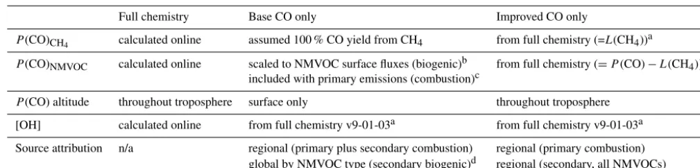
In subsequent sections, we compare CO from three GEOS-Chem simulations (Table 1): (1) a “standard full chemistry” run that simulates the full suite of chemical species in the GEOS-Chem mechanism (including CO) and their coupled production and loss; (2) a “base CO-only” run that uses the standard CO-only capability included in GEOS-Chem v9-01-03 (with minor modifications described below); and (3) an “improved CO-only” run that incorporates the modi-fications described in this work. For all simulations, we use a horizontal resolution of 2◦×2.5◦ with model time steps of 15 min for transport and 60 min for chemistry. Biomass burning CO emissions are from GFEDv3 and anthropogenic emissions are from EDGARv3.2 (fossil fuels) and Yevich and Logan (2003) (biofuels), with regional overwrites as de-tailed in Fisher et al. (2010). We simulate a 3-year period
(2009–2011) to understand the influence of interannual vari-ability on our results.
2.2 CO-only simulation in GEOS-Chem
Linear CO-only simulation (also known as “tagged CO”) has been a capability included in the GEOS-Chem CTM since version 2-08 (http://acmg.seas.harvard.edu/geos/geos_ versions.html). The code for the CO-only simulation (as well as other speciality simulations) is embedded in the standard GEOS-Chem code, with the choice of simulation selected at runtime. Hence, version numbers for the CO-only simulation are the same as for the full GEOS-Chem release. In what fol-lows, the “base” CO-only simulation refers to v9-01-03, with minor modifications as described below.
The CO simulation operates as follows. In a given model grid box, the rate of change in the CO concentration ([CO]) due to emissions and chemistry is given by
d[CO]
dt =E+P (CO)−k[OH][CO], (1)
where E represents surface emissions, P(CO) repre-sents chemical production of CO from methane and non-methane volatile organic compounds (NMVOCs), [OH] is the OH concentration, and k represents the pressure- and temperature-dependent rate constant for oxidation of CO by OH from the Jet Propulsion Laboratory (JPL) data evaluation (Burkholder et al., 2015). In Eq. (1) we neglected transport to and from neighboring grid boxes since our focus here is on the influence of the chemistry, but the effects of advec-tion are accounted for in the model. Surface emissions come from external inventories, as described in Sect. 2.1. In the standard GEOS-Chem simulation, P(CO) and k[OH][CO] in Eq. (1) would be coupled to the concentrations of other chemical species (methane, NMVOCs, and OH, each repre-sented by similar differential equations) using a chemistry solver. In contrast, the CO-only simulation is run in a chemi-cally offline mode, in which the simulation is decoupled from the chemistry solver.
systemat-Table 1.Chemical production, loss, and source attribution details for simulations performed in this work.
Full chemistry Base CO only Improved CO only
P(CO)CH4 calculated online assumed 100 % CO yield from CH4 from full chemistry (=L(CH4))a
P(CO)NMVOC calculated online scaled to NMVOC surface fluxes (biogenic)b from full chemistry (=P (CO)−L(CH4))a
included with primary emissions (combustion)c
P(CO) altitude throughout troposphere surface only throughout troposphere
[OH] calculated online from full chemistry v9-01-03a from full chemistry v9-01-03a
Source attribution n/a regional (primary plus secondary combustion) regional (primary combustion)
global by NMVOC type (secondary biogenic)d regional (secondary, all NMVOCs)
aArchived fields from full chemistry simulation are used as monthly mean values.
bAssumed CO yields are 100 % from methanol, 67 % from acetone, 30 % from isoprene, and 20 % from monoterpenes. cCalculated by scaling primary fossil fuel emissions by 19 % and primary biomass burning emissions by 11 %. dFor methanol, acetone, isoprene, and monoterpenes only.
ically lower when using the updated OH fields, as shown in Fig. S1 in the Supplement.
The chemical production term (P(CO)) requires special treatment, as it depends on the time-varying concentrations of methane and NMVOC precursors. This term is treated dif-ferently in the base and improved versions of the CO-only simulation, as described in detail in Sect. 2.2.1 and 2.2.2.
We also fixed a few minor problems in the v9-01-03 CO-only simulations to bring them up to date with the current public version (v11-01) and to make them more compatible with the full chemistry simulation. Specifically, we imple-mented optional non-local mixing in the planetary boundary layer (Lin and McElroy, 2010) and the centralized chemistry time step (http://wiki.seas.harvard.edu/geos-chem/index. php/Centralized_chemistry_time_step) – both of which are defaults in the v9-01-03 standard full chemistry simulation but were missing from the CO-only simulation. We also added diurnal scaling of the monthly mean [OH] fields based on the cosine of the solar zenith angle. This is the same method used in all other offline simulations in GEOS-Chem, and it is an objective improvement to use of a single monthly mean value in each grid box. All of these updates are included in both the base and improved versions compared below.
2.2.1 Original (base) CO-only simulation
In the original CO-only model, subsequently re-ferred to as the base simulation, CO is produced chemically from five precursors: methane, acetone, methanol, isoprene, and monoterpenes. In other words,
P (CO)=P (CO)methane+P (CO)acetone+P (CO)methanol+
P (CO)isoprene+P (CO)monoterpenes. For methane, the model assumes a 100 % molar CO yield from oxidation by OH, with methane concentrations defined as averages of surface observations from NOAA carbon cycle surface flasks over four latitudinal bands (30–90◦N/S, 0–30◦N/S). These assumptions are applied throughout the troposphere.
For NMVOC precursors, CO production occurs in the model surface layer only (i.e., it is treated as an additional emission), with assumed molar yields of 67 % from acetone, 100 % from methanol, 30 % from isoprene, and 20 % from monoterpenes (Duncan et al., 2007). Isoprene and monoter-pene emissions are from the Model of Emissions of Gases and Aerosols from Nature (MEGAN), as in the standard full chemistry simulation. Acetone emissions come from Jacob et al. (2002), and the methanol flux is scaled to the isoprene flux assuming a methanol-to-isoprene molar ratio of∼1:4. Acetone and methanol are therefore decoupled from the full chemistry simulation and do not take into account recent up-dates to their budgets (e.g., Fischer et al., 2012; Wells et al., 2014). CO production from NMVOCs emitted during com-bustion is accounted for by increasing primary CO emissions from anthropogenic and biomass burning sources by 19 and 11 %, respectively (Duncan et al., 2007). As for the biogenic NMVOC source, this production is applied directly in the surface layer.
2.2.2 Improved CO-only simulation
in the Supplement, interannual variability in simulated CO is dominated by variability in the meteorology and primary emissions with only a very minor contribution from variabil-ity in the CO production rates (Sect. S1, Figs. S2 and S3). However, the code is designed in such a way that an inter-ested user could easily re-run the standard chemistry simula-tion to save the CO producsimula-tion fields for a specific year of in-terest. This extra step would generally only be necessary for changes likely to significantly impact chemical production (for example, different biogenic emissions or meteorological fields).
The total P(CO) saved from the full chemistry model is split offline into contributions from methane (P (CO)CH4) and from NMVOCs (P (CO)NMVOC) by also saving the methane loss rates (L(CH4)) from the full chemistry simu-lation. We maintain the assumption from the original CO-only simulation of a 100 % CO yield from methane oxida-tion, such that P (CO)CH4=L(CH4). The NMVOC contri-bution is then the difference between the total CO production and the methane contribution: P (CO)NMVOC=P (CO)−
P (CO)CH4. The assumption of a 100 % CO yield will some-what overestimate the contribution from methane relative to the contribution from NMVOCs. This mainly affects the tropical lower troposphere, where we occasionally find that methane loss exceeds total CO production, likely due to rapid vertical transport of intermediate products. Scaveng-ing of soluble intermediate products (for example, methyl hydroperoxide) also reduces the CO yield from methane, al-though this is expected to be a small effect (e.g., <0.1 % in our 1-day tests for methyl hydroperoxide). In the few cases where P (CO)CH4 overestimates totalP(CO), we cap
P (CO)CH4at the total CO production rate. This assumption does not affect the total CO production, retaining consistency with the standard full chemistry simulation.
The saved CO production fields (P (CO)CH4 and
P (CO)NMVOC) are then used as input to the linear CO-only model:
d[CO]
dt =E+P (CO)CH4+P (CO)NMVOC−k[OH][CO]. (2)
This is similar to the approach used for the GEOS-Chem tagged odd oxygen simulation (Li et al., 2002). The archived fields are scaled diurnally using the cosine of the solar zenith angle, as is done for OH concentrations in GEOS-Chem and for source profiles in other models (e.g., the model intercom-parison of Zeng et al., 2015). Our updated treatment is ap-plied in a flexible manner that allows a user to choose the original CO production method (scaling surface emissions) if so desired.
2.2.3 Source attribution capability
In both the base and improved simulations, Eq. (1) is lin-ear in [CO]. As a result of this linlin-earity, CO from different sources and regions can be treated independently (referred to
as tagged CO tracers; Bey et al., 2001). For primary emitted CO, Eq. (1) becomes
d[COi,j]
dt =Ei,j−k[OH][COi,j], (3)
where i represents the emission type (e.g., fossil fuel, biomass burning),j the geographical region in which that source is emitted, and [COi,j] is a separate CO tracer for
each emission type and geographical region.
For secondary chemically produced CO, the treatment dif-fers between the two model versions. In the base model, sec-ondary CO is distinguished by the precursor NMVOC but not by region, such that Eq. (1) becomes
d[COm,global]
dt =P (CO)m,global−k[OH][COm,global], (4)
wherem represents the precursor (i.e., acetone, methanol, isoprene, or monoterpenes). In the improved model, we can no longer distinguish between different NMVOCs. Instead, we now tag secondary CO from NMVOCs by the geograph-ical region where production occurs, similar to the tagging used for primary CO emissions, such that Eq. (1) becomes
d[CONMVOC, j]
dt =P (CO)NMVOC, j−k[OH][CONMVOC, j]. (5) In other words, CONMVOC, jfrom regionjrepresents the CO
that was produced within the boundaries of regionj, regard-less of the origin of the NMVOC (i.e., local vs. transported). As most precursor NMVOCs have short atmospheric life-times, most CONMVOC, j will derive from NMVOCs
emit-ted in regionj. While the improved method does not allow us to distinguish between production from different precur-sor NMVOCs (e.g., isoprene vs. monoterpenes) or types of NMVOC emissions (e.g., biogenic vs. anthropogenic), we find that by combining these regional secondary CO trac-ers with the primary CO tractrac-ers we are usually able to infer the likely source of secondary enhancements. An example is discussed in Sect. 5. In both base and improved simulations, secondary CO produced from methane is carried as a single, global tracer.
3 Implications for global CO distribution
Surf ace
-10 -5 0 5 10 ppbv 500 hPa
Improved CO-only – f ull chemistry Base CO-only – f ull chemistry
-50 -25 0 25 50 ppbv
(a) (b)
(c) (d)
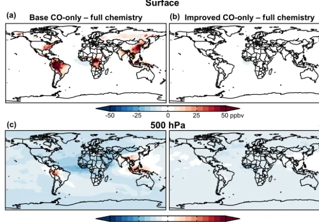
Figure 1.July 2009 surface(a, b)and 500 hPa(c, d)maps of the biases in the CO mixing ratio in the CO-only simulations relative to the full chemistry simulation (used here as reference). Panels(a, c)show biases in the base CO-only simulation and panels(b, d)show biases in the improved CO-only simulation. The main difference between the two CO-only simulations is the vertical distribution of the CO source from NMVOCs, which is three-dimensional in the improved simulation but only occurs in the surface layer in the base simulation.
Indonesia, and the southeast US). Similar, smaller (up to 50 ppbv/10–15 %) effects are present in regions with elevated NMVOC emissions from anthropogenic and biomass burn-ing sources (e.g., China, Alaska). These overestimates reflect the assumed instantaneous CO production from VOCs in the surface layer in the base model, whereas in the full chemistry and updated models this production happens more gradually. As a result, the high bias over continents in the base simu-lation is balanced by a low bias in continental outflow (e.g., the west African plume), at higher altitudes, and in remote regions where there is delayed production following trans-port.
At 500 hPa, the base CO-only simulation underestimates the full chemistry simulation across much of the globe, again due to delayed CO production during transport. These dif-ferences are generally much smaller (4–5 ppbv/4–7 %) than at the surface, reflecting the more widespread nature of sec-ondary production. In a few regions (central Amazon, In-donesia, and southern China), the base CO-only simula-tion actually overestimates the full chemistry simulasimula-tion at 500 hPa by 7–8 ppb (10–12 %). These are regions where large NMVOC sources are coupled with frequent deep vective activity. In the full chemistry simulation, deep con-vection rapidly transports CO precursors to high altitude, and CO production is offset to the middle and upper troposphere (Fisher et al., 2015). In the base CO-only simulation, how-ever, the CO is already present in surface air, and it is CO itself rather than the precursors that is transported to higher altitudes.
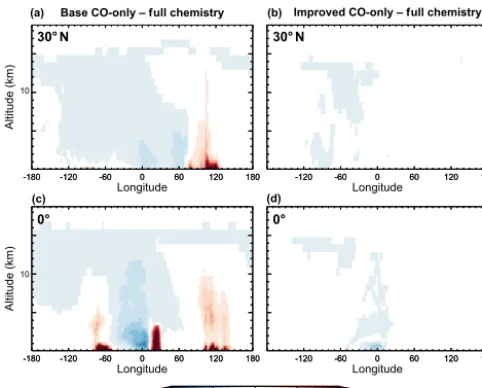
The impacts on the vertical distribution are more clearly seen in Fig. 2, which shows longitudinal cross sections at the Equator and at 30◦N, and in Fig. 3, which shows latitudinal cross sections at 60◦W and 0◦E. Consistent with the maps in Fig. 1, the cross sections show that the base simulation overestimates CO over continental source regions from the surface to as high as 5 km over South America and Africa, and as high as 10–12 km over Indonesia and China. As seen previously, the high biases over source regions are coupled with low biases in downwind outflow regions.
-20 -10 0 10 20 ppbv -180 -120 -60 0 60 120 180
Longitude 10
Altitude (km)
-180 -120 -60 0 60 120 180 -180 -120 -60 0 60 120 180
Longitude
Altitude (km)
-180 -120 -60 0 60 120 180 10
-120 -60 0 60 120 180 Longitude
-120 -60 0 60 120 180
30°N 30°N
0°
-120 -60 0 60 120 180 Longitude
-120 -60 0 60 120 180 0°
Improved CO-only – f ull chemistry Base CO-only – f ull chemistry
(a) (b)
(c) (d)
Figure 2.July 2009 longitude–altitude cross sections at 30◦N(a, b) and 0◦(c, d)of the biases in CO mixing ratio in the CO-only simu-lations relative to the full chemistry simulation (used here as refer-ence). Panels(a, c)show biases in the base CO-only simulation and panels(b, d)show biases in the improved CO-only simulation.
4 Implications for global evaluation with observations
We use a global dataset of ground-based and airborne CO observations to evaluate the improved CO-only simulation in reference to the base simulation and the standard chemistry simulation. As in Sect. 3, we show model output from 2009, which is virtually identical to output from our other simu-lation years (2010 and 2011). The observations are the same data used to benchmark new versions of the full GEOS-Chem model (http://acmg.seas.harvard.edu/geos/geos_benchmark. html), and the software to perform the evaluation is a modi-fied version of the full benchmarking code (https://bitbucket. org/gcst/gc_1yr_benchmark/). A version of the CO-only benchmarking code and relevant observations are available at https://github.com/jennyfisher/CO_Benchmark. The bench-mark evaluation produces over 200 plots, of which represen-tative examples are provided in Fig. S6. The full set of plots, including for other simulations years, is also included in the Supplement.
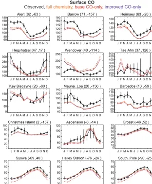
Figure 4 compares the base and updated CO-only and full chemistry simulations to observations at a subset of the sites in the NOAA Global Monitoring Division (GMD) network. The largest differences between the two CO-only simulations are seen at the northern midlatitude continental sites (e.g., up to 20 ppbv over Wendover, Utah, USA; 27 ppbv in Hegy-hátsál, Hungary; 47 ppbv over Tae Ahn, South Korea), but in all cases these differences are significantly smaller than the observation–model mismatch. On a relative scale, differ-ences are largest at the Antarctic sites (up to 15 %), where they are sufficient to improve agreement with the observa-tions. No sites are located in the major biogenic NMVOC
-20 -10 0 10 20 ppbv
Improved CO-only – f ull chemistry Base CO-only – f ull chemistry
Al
tit
ud
e
(k
m
)
10
-90 -60 -30 0 30 120 90 Latitude
Al
tit
ud
e
(k
m
)
10
60° W 60° W
0° E 0° E
-90 -60 -30 0 30 120 90 Latitude
-90 -60 -30 0 30 120 90
Latitude -90 -60 -30 Latitude0 30 120 90
(a) (b)
(c) (d)
Figure 3.July 2009 latitude–altitude cross sections at 60◦W(a, b) and 0◦E(c, d)of the biases in CO mixing ratio in the CO-only simulations relative to the full chemistry simulation (used here as reference). Panels(a, c)show biases in the base CO-only simulation and panels(b, d)show biases in the improved CO-only simulation.
Alert (82 ,-63 )
Surface CO
Observed, full chemistry, base CO-only, improved CO-only
J F M A M J J A S O N D 60
80 100 120 140 160
180 Barrow (71 ,-157 )
J F M A M J J A S O N D 60
80 100 120 140 160
180 Heimaey (63 ,-20 )
J F M A M J J A S O N D 60
80 100 120 140 160
Hegyhatsal (47 ,17 )
J F M A M J J A S O N D 100
150 200 250 300
Wendover (40 ,-114 )
J F M A M J J A S O N D 100
150 200
250 Tae Ahn (37 ,126 )
J F M A M J J A S O N D 150
200 250 300 350 400 450 500
Key Biscayne (26 ,-80 )
J F M A M J J A S O N D 0
50 100 150
Mauna_Loa (20 ,-156 )
J F M A M J J A S O N D 40
60 80 100 120
140 Barbados (13 ,-59 )
J F M A M J J A S O N D 50
60 70 80 90 100 110 120
Christmas Island (2 ,-157 )
J F M A M J J A S O N D 0
20 40 60 80
100 Ascension (-8 ,-14 )
J F M A M J J A S O N D 40
60 80 100
120 Crozet (-46 ,52 )
J F M A M J J A S O N D 0
10 20 30 40 50 60 70
Syowa (-69 ,40 )
J F M A M J J A S O N D 30
40 50 60
70 Halley Station (-76 ,-26 )
J F M A M J J A S O N D 30
40 50 60
70 South_Pole (-90 ,-25 )
J F M A M J J A S O N D 30
40 50 60 70
Figure 4.Observed and modeled CO seasonal cycle in surface air from a subset of sites in the GEOS-Chem benchmark dataset. Additional site comparisons can be seen in the full benchmark evaluations included in the Supplement. Sites are ordered from top left to bottom right by latitude, with coordinates for each given as (◦N,◦E). Both observations and model results are for the year 2009. Observations are shown in black as monthly means and standard deviations. Model results are monthly means at the location of each site from the full chemistry (solid orange), base CO-only (dashed red), and improved CO-only (dashed purple) simulations. The main difference between the two CO-only simulations is the vertical distribution of the CO source from NMVOCs, which is three-dimensional in the improved simulation but only occurs in the surface layer in the base simulation.
Yoon and Pozzer, 2014; Strode et al., 2016). The full GEOS-Chem benchmark is similarly conducted for a much more recent year (2013), and updating the benchmark dataset to include more recent airborne observations, including those in regions sensitive to biogenic emissions and chemical produc-tion, should be a priority for the GEOS-Chem community.
We also evaluated the simulation using quantitative met-rics derived from airborne data that describe the CO seasonal cycle (first harmonic) and vertical profile (polynomial terms) in the remote Southern Hemisphere (see Fisher et al., 2015 for details). The resulting coefficients are given in the Sup-plement (Figs. S8 and S9). Consistent with the results above, the fit parameters for the full chemistry simulation are more closely approximated by the improved CO-only simulation
than the base version; however, the changes do not signifi-cantly impact the match to the observed parameters. Addi-tional Southern Hemisphere evaluation specific to the Aus-tralasian region is provided in the next section.
New Guinea (PEM WB)
40 60 80 100 120
Feb 1994
1000 800 600 400
200 Amazon (ABLE-2A)
40 90 140 190 240
Aug 1985
1000 800 600 400
200 Amazon (ABLE-2B)
40 75 110 145 180
May 1987
1000 800 600 400 200
CO (ppb)
Pressure (hPa)
CO vertical profiles
Observed, full chemistry, base CO-only, improved CO-only
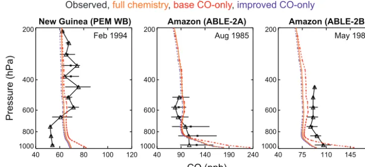
Figure 5.Observed and modeled CO vertical profiles from a subset of aircraft campaigns in the GEOS-Chem benchmark dataset. Obser-vations are shown in black with model results for 2009 from the full chemistry (solid orange), base CO-only (dashed red), and improved CO-only (dashed purple) simulations. The month and year during which the aircraft data were collected are provided inset. Additional aircraft comparisons can be seen in Fig. S7 and in the full benchmark evaluations included in the Supplement.
(Figs. 1–3). Consistent with the rest of the evaluation, we find that the improved simulation provides a marginally better simulation of the observations, but the improvement (∼1 %) is much smaller than the model bias relative to IASI (∼18 %) (not shown given the small impact of the simulation change).
5 Implications for source attribution: case study for Australasia
Our improved CO-only simulation includes for the first time in GEOS-Chem the ability to geographically tag secondary CO from NMVOC oxidation (see Sect. 2.2.3). Previously, geographic tagging was only available for direct emissions from fossil fuel and biofuel combustion and biomass burn-ing. Outside of the Northern Hemisphere extratropics, direct emissions are generally responsible for only a small fraction of CO (Duncan et al., 2007; Pfister et al., 2008; Zeng et al., 2015), and so tagging direct emissions only is insufficient for understanding CO or air mass origin. This is especially true in the Southern Hemisphere tropics and midlatitudes, where anthropogenic emissions are low and biogenic emissions are large.
To illustrate the new tagging capabilities and their impli-cations, we perform a case study for the Australasian re-gion (Australia and New Zealand). Like much of the South-ern Hemisphere extratropics, Australasia is characterized by very low anthropogenic emissions coupled with episodically high biomass burning emissions in austral spring (October– November; Edwards et al., 2006). Biogenic emissions are also expected to be large in austral summer (December– February) in northern and southeastern Australia (Guenther et al., 2012; Bauwens et al., 2016), although the magnitude
of the biogenic enhancement remains uncertain (Emmerson et al., 2016). As local emissions are generally low, Aus-tralasian tropospheric composition is frequently impacted by intercontinental transport of air masses from elsewhere in the Southern Hemisphere (Gloudemans et al., 2006; Zeng et al., 2012; Buchholz et al., 2016). Significant attention has been paid to transported biomass burning plumes (e.g., Pak et al., 2003; Gloudemans et al., 2006; Edwards et al., 2006; Zeng et al., 2012). However, recent work by Buchholz et al. (2016) and Té et al. (2016) suggests that NMVOC oxidation dom-inates over biomass burning as a CO source throughout the year in the Australian extratropics and in all months except September–October in the tropics. The origin and impact of transport from biogenic source regions in Australasia has not previously been explored.
We evaluate the CO source attribution in Australasia at three locations spanning a range of Southern Hemisphere environments: a tropical site in Darwin, Australia (12.4◦S, 130.9◦E), a midlatitude site near the Sydney metropolitan area in Wollongong, Australia (34.4◦S, 150.9◦E), and a re-mote site with minimal anthropogenic influence in Lauder, New Zealand (45.0◦S, 169.7◦E). All three sites make total
column measurements of CO as part of the TCCON (Wunch et al., 2011) and the Network for the Detection of Atmo-spheric Composition Change (NDACC). Total column CO measurements have previously been compared to the stan-dard GEOS-Chem simulation by Zeng et al. (2015) at all three sites (using the NDACC record) and by Té et al. (2016) over Wollongong (using both NDACC and TCCON records). Here, we use the TCCON data only.
CO, in molecules cm−2, using total column O2,O2:
CO=10−9XCO·
O2
0.2095. (6)
O2 is calculated from variables available in the standard public TCCON files includingp(pressure, in hPa) andXH2O (column-averaged water vapor, in ppm), along with an ancil-lary product created during TCCON data processing called
Xair (the ratio between the calculated pressure-derived and retrieved dry air columns) as follows:
O2 =0.2095·10
−2× pNA
Mairg
× 1
Xair+10−6XH2O
, (7)
whereNAis Avogadro’s constant,Mairis the molar mass of air in kg mol−1,gis the gravitational constant in m s−2, and 10−2and 10−6are unit conversion terms.
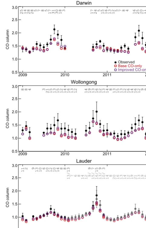
Figure 6 compares total column CO from the improved (purple) and base (red) GEOS-Chem CO-only simulations to the TCCON observations (black/gray) from 2009 to 2011 at the three sites. Consistent with the previous sections, differ-ences between the two CO-only simulations are small. The improved CO-only simulation is in general somewhat higher than the base simulation, especially over Lauder, implying that the CO column is primarily sensitive to transported CO in the free troposphere rather than to local surface sources, as expected. As seen in previous comparisons (Zeng et al., 2015; Té et al., 2016), GEOS-Chem underestimates the total column at all sites, with the best agreement over Lauder.
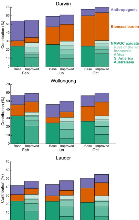
The CO source attribution from both the base and im-proved model versions is illustrated in Fig. 7 for 2009. The figure shows three months selected to sample different source influences: February (austral summer), when large biogenic emissions are expected in northern and southeastern Aus-tralia as well as upwind continents; June (austral winter), the start of the dry (burning) season in Darwin but with minimal biogenic and biomass burning emissions elsewhere; and Oc-tober (austral spring), a period with near-peak biomass burn-ing across much of the Southern Hemisphere. Contributions are shown from anthropogenic (fossil fuel plus biofuel) emis-sions (purple), biomass burning (orange), and oxidation of NMVOCs (green), with the remaining CO from methane ox-idation (not shown but equivalent to the difference between 100 % and the sum of the stacked contributions). For clarity, the anthropogenic and biomass burning contributions from different regions have been summed globally. The new ca-pability to distinguish regional signatures in the NMVOC source is highlighted for the improved model with different shading. The sensitivity of the source attribution to interan-nual variability inP(CO) is shown in Fig. S3.
Figure 7 shows that the contribution from NMVOC oxi-dation dominates over the emitted primary CO at the mid-latitude sites, with the two approximately equal over Dar-win. In all cases, the improved simulation shows a larger contribution from NMVOC oxidation than in the base sim-ulation. This is in part due to a change in the treatment of
Darwin
2009 2010 2011 2012
0.5 1.0 1.5 2.0 2.5 3.0
CO column
25 14 28 28 5 7 8 5 17 31 30 18 3 17 24 5 15 16 13 12 5 7 8 4 16 25 20 11
Wollongong
2009 2010 2011 2012
0.5 1.0 1.5 2.0 2.5 3.0
CO column
8 8 4 3 21 15 13 15 12 14 16 13 12 14 19 13 16 12 13 14 8 13 15 13 12 16 14 16 12 9 9
Lauder
2009 2010 2011 2012
0.5 1.0 1.5 2.0 2.5 3.0
CO column
11 2 9 13 10 6 10 12 10 14 8 8 13 9 7 15 9 3
13/ 7 6 8 14 12 9/ 15/ 16/ 13/ 10/ 14 8 20 16 13 14 12 19 21 13 19 15 Observed B ase CO-only I mproved CO-only
Figure 6.Observed and modeled time series of 2009–2011 monthly mean CO total columns in the Australasian region. Observations from the TCCON sites in Darwin (12.4◦S, 130.9◦E; Griffith et al., 2014a), Wollongong (34.4◦S, 150.9◦E; Griffith et al., 2014b), and Lauder (45.0◦S, 169.7◦E; Sherlock et al., 2014a, b) are shown in black as monthly means and standard deviations of all data within each month, with the number of days of data in each month given as the inset in the figures. Simulated daily mean CO from the base CO-only (red) and improved CO-only (purple) simulations has been sampled from the relevant grid boxes only for days with avail-able observations and smoothed using observed averaging kernels. For Lauder, the spectrometer changed from a Bruker 120HR (dark points/counts) to a Bruker 125HR (light points/counts); both mea-surements are shown for periods of overlapping data availability. For site locations, see Fig. 8.
Wollongong
Lauder
Base
FebImproved Jun Oct
0 10 20 30 40 50 60 70
C
on
tri
bu
tio
n
(%
)
Improved Improved
Base Base
Darwin
Feb Jun Oct
0 10 20 30 40 50 60 70
C
on
tri
bu
tio
n
(%
)
Base Improved Base Improved Base Improved
Feb Jun Oct
0 10 20 30 40 50 60 70
C
on
tri
bu
tio
n
(%
)
Base Improved Base Improved Base Improved
Anthropogenic
Biomass b urning
NMVOC oxidation: R est of the world Indonesia Africa S. America Australasia
Figure 7.Simulated contributions of different sources to total sim-ulated CO at the Australasian TCCON sites in 2009 (see Fig. 8 for site locations). The figure compares the base (left bars) and improved (right bars) CO-only simulations at the TCCON sites at three times of the year: February (left, austral summer); June (middle, austral winter); and October (right, peak Southern Hemi-sphere biomass burning). Colored bars show the percent contri-butions from anthropogenic emissions (purple), biomass burning emissions (orange), and secondary production from NMVOC ox-idation (green). The remainder comes from methane oxox-idation. For the NMVOC source, the contributions in the improved simulation are divided into source regions (from darkest to lightest): Australa-sia (112.5–180◦E, 48–10◦S), South America (120–30◦W, 58◦S– 15◦N), Africa (30◦W–60◦E, 36◦S–36◦N), Indonesia (95–165◦E, 10◦S–6◦N), and the rest of the world. Note that the region def-initions include some ocean areas to capture continental outflow, but the majority of the NMVOC production happens over the conti-nents.
figure also shows that this cannot explain the entirety of the difference, as the sum of the non-methane contributions (an-thropogenic plus biomass burning plus NMVOC oxidation)
is consistently larger in the improved simulation. The differ-ence is particularly large over Lauder, where the infludiffer-ence from primary emissions is generally small. This suggests the improved simulation corrects a consistent underestimate of secondary production found in the base CO-only simulation, with the largest impact in remote regions downwind of bio-genic sources.
The source attribution of the NMVOC oxidation term pro-vided in the improved model (Fig. 7, right bars) shows that the TCCON sites are sensitive to secondary CO produced in a diverse range of environments, including not only Aus-tralasia but also South America, Africa, and (over Darwin) Indonesia. Biogenic emissions of CO precursors in our sim-ulations are from the MEGAN model, which estimates very high and likely overestimated isoprene across most of north-ern Australia (Guenther et al., 2012; Bauwens et al., 2016), including the region surrounding the Darwin site. Despite the magnitude of these emissions, we find that typically less than half of the NMVOC source over Darwin is local to Aus-tralia. At the midlatitude sites, transported CO produced from South American and African NMVOCs provides a large con-tribution to the column, especially outside of austral sum-mer (>10 %). The ability to disaggregate these different contributions can aid in future interpretation of the TCCON data from these sites, including for co-measured species like methane and carbon dioxide.
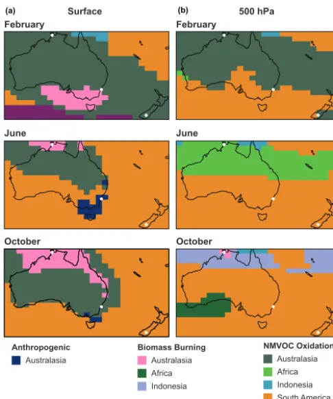
More generally, Fig. 8 shows the dominant non-methane contribution to surface and 500 hPa CO over Australasia in February, June, and October. At the surface, oxidation of Australian NMVOCs dominates the CO burden over much of the Australian continent, and in February this dominance extends horizontally to New Zealand and vertically to the free troposphere. As noted previously, this is likely due to the large estimated biogenic emissions in austral summer. We see also from Fig. 8 that transported CO produced from South American NMVOC emissions typically dominates the Aus-tralasian background (complemented by a similar contribu-tion from African NMVOC oxidacontribu-tion in northern Australia in June). Even in October, at the height of the Southern Hemi-sphere burning season, transported chemically produced CO dominates over primary CO (local or transported) in the free troposphere. We note that there is significant interannual variability in source dominance in October, with a larger con-tribution from African biomass burning in 2011 and a much larger contribution from South American biomass burning in 2010. In other months, there is limited interannual variabil-ity, and the dominant contributions are very similar to those presented here.
Surface 500 hPa
February February
June June
October October
Australasia
Anthropogenic
Australasia
Biomass Burning
Africa Indonesia
Australasia
NMVOC Oxidation
Africa Indonesia South America Other
(a) (b)
Figure 8. GEOS-Chem simulation of the dominant non-methane
contribution to Australasian CO at the surface(a)and at 500 hPa(b) in three months, using the improved CO-only simulation with CO source tagged by both type (anthropogenic, biomass burning, or NMVOC oxidation) and region of emissions/production (with re-gional boundaries the same as in Fig. 7). White circles show the locations of the TCCON sites used in Figs. 6 and 7.
simulate observed CO vertical gradients over the Southern Ocean. These could not be explained by primary CO and were therefore attributed to differences in secondary CO, pri-marily produced from biogenic NMVOC emissions in South America. However, the authors could not unambiguously de-convolve the effects of differences in chemical production versus differences in transport. Tagging the secondary CO by region of production in the different models would have al-lowed a quantitative analysis of differences in transport ver-sus production. Implementation of this capability in multi-ple models could pave the way for improved interpretation of multi-model comparisons, especially those focused on re-mote regions.
6 Conclusions
We have implemented a major improvement to the represen-tation of secondary CO production in the GEOS-Chem linear “tagged” CO-only simulation, which is frequently used for emission inversion, data interpretation, and chemical
fore-casting. The improvement targets the production of CO from non-methane volatile organic compounds (NMVOCs), which was previously scaled to NMVOC emissions (assuming fixed yields) and injected into the model surface layer only. This resulted in a decoupling between the full chemistry and CO-only simulations in both the magnitude and location of sec-ondary CO production. The improved simulation remedies both problems.
In the improved CO-only model, we now use archived CO chemical production rates from the full chemistry sim-ulation, ensuring consistency between the two simulations. We use the methane loss rate (also archived from the full chemistry simulation) to distinguish between CO produced from methane oxidation and that produced from NMVOCs. The latter contribution is for the first time tagged by the ge-ographical region where the production occurs, providing a more comprehensive understanding of air mass origin.
Using the full chemistry simulation as a reference, we showed that the base CO-only simulation greatly overesti-mates CO in the model surface layer, especially over bio-genic source regions (by more than 100 ppbv), due to the assumption of instantaneous surface production. In regions where biogenic emissions coincide with deep convective activity (e.g., South America, Indonesia), the overestimate is expressed throughout much of the troposphere. This re-flects the fact that it is typically NMVOCs and/or their in-termediate oxidation products that are lifted from the surface layer, with CO production largely happening downwind. The model overestimates at the surface and over major source re-gions are paired with more diffuse underestimates in outflow regions. Both overestimates and underestimates are largely resolved in the improved CO-only simulation, which shows much closer agreement with the full chemistry.
The improved CO-only simulation includes a new capa-bility to geographically tag secondary CO by the region where production occurs. To illustrate this capability, we per-formed a case study for the Australasian region, where CO is dominated by secondary production. We found that ob-served total column CO at three TCCON sites across Aus-tralasia (Darwin, Wollongong, and Lauder) is sensitive to secondary CO from a range of sources. Throughout much of the year, transported secondary CO dominates over sec-ondary CO produced within Australia, despite large biogenic emissions there, with particularly large contributions from South America, followed by Africa and (in the north) Indone-sia. Even at the height of the austral biomass burning season that has been the focus of most analysis of intercontinental transport in the Southern Hemisphere, we show that trans-ported secondary CO from NMVOC oxidation can outweigh transported primary CO from biomass burning.
Linear “tagged” CO-only simulations are used across the atmospheric chemistry community and are of particular value for interpreting field observations and understanding variation in multi-model ensembles. While tagging is gen-erally reserved for primary emissions, secondary production dominates the CO budget throughout much of the world and especially in the Southern Hemisphere. Because much of that secondary source comes from oxidation of NMVOCs that are enhanced in biogenic source regions and low elsewhere, there is a geographic signature to secondary CO that can aid in interpretation of observations and model results. We rec-ommend that future attribution studies in regions where pri-mary emissions are low follow the methods described here to include source attribution of secondary CO contributions.
Code availability. The standard GEOS-Chem code is freely
ac-cessible to the public by following the guidelines at http://wiki. geos-chem.org/. Updates described here will be included in the standard code once this paper has been accepted, likely after version 11-02. In the interim, the version 9-01-03 code used here is available at https://github.com/jennyfisher/GEOS-Chem_ TaggedCO_v9.01.03_updated. The standard GEOS-Chem code is distributed as a Git repository, and the code updates described here can be added to a standard v9-01-03 code repository by pulling the branch linked above. The provisional version of v11-01 where we have implemented these updates is available by contacting the authors. Instructions for running the GEOS-Chem model, includ-ing the CO-only simulation, are provided in the GEOS-Chem user guide: http://acmg.seas.harvard.edu/geos/doc/man/.
The CO-only benchmark code is a condensed and slightly adapted version of the standard GEOS-Chem 1-year benchmark code, available at https://bitbucket.org/gcst/gc_1yr_benchmark/. The CO-only version of the benchmarking code (including the CO observations used to evaluate the model) is available at https: //github.com/jennyfisher/CO_Benchmark.
Author contributions. JAF, LTM, and DBAJ formulated the method
for the improved simulation. JAF developed the model code with contributions from LTM and DBAJ, performed the simulations, and conducted the analysis. NMD provided the methodology for con-verting the TCCON data fromXCOtoCO. JAF prepared the pa-per with contributions from all authors.
Competing interests. The authors declare that they have no conflict
of interest.
Acknowledgements. This work was funded by a University of
Wol-longong Vice Chancellor’s Postdoctoral Fellowship to J. A. Fisher with the assistance of resources provided at the NCI National Facility systems at the Australian National University through the National Computational Merit Allocation Scheme supported by the Australian Government. N. M. Deutscher is supported by ARC-DECRA grant DE140100178. TCCON data from Wollongong and Darwin are supported by NASA grants NAG5-12247 and NNG05-GD07G, and Australian Research Council grants DP140101552, DP110103118, DP0879468, and LP0562346. Technical support for TCCON measurements at Darwin from the Bureau of Meteorology, and formerly the DOE ARM program, is gratefully acknowledged. The Lauder TCCON program is core-funded by NIWA through the New Zealand Ministry of Business, Innovation and Employment. We thank Rebecca Buchholz and Clare Paton-Walsh for helpful discussions in the initial stages of this work, and Voltaire Velazco and Dave Pollard for providing the ancillary TCCON variables not available in the public files.
Edited by: Volker Grewe
Reviewed by: two anonymous referees
References
Bauwens, M., Stavrakou, T., Müller, J.-F., De Smedt, I., Van Roozendael, M., van der Werf, G. R., Wiedinmyer, C., Kaiser, J. W., Sindelarova, K., and Guenther, A.: Nine years of global hydrocarbon emissions based on source inversion of OMI formaldehyde observations, Atmos. Chem. Phys., 16, 10133– 10158, https://doi.org/10.5194/acp-16-10133-2016, 2016. Bey, I., Jacob, D. J., Logan, J. A., and Yantosca, R. M.:
Asian chemical outflow to the Pacific in spring: Origins, pathways, and budgets, J. Geophys. Res., 106, 23097–23113, https://doi.org/10.1029/2001JD000806, 2001.
Buchholz, R., Paton-Walsh, C., Griffith, D., Kubistin, D., Caldow, C., Fisher, J., Deutscher, N., Kettlewell, G., Riggenbach, M., Macatangay, R., Krummel, P., and Langenfelds, R.: Source and meteorological influences on air quality (CO, CH4& CO2) at a Southern Hemisphere urban site, Atmos. Environ, 126, 274–289, https://doi.org/10.1016/j.atmosenv.2015.11.041, 2016.
Chen, Y., Li, Q., Randerson, J. T., Lyons, E. A., Kahn, R. A., Nel-son, D. L., and Diner, D. J.: The sensitivity of CO and aerosol transport to the temporal and vertical distribution of North Amer-ican boreal fire emissions, Atmos. Chem. Phys., 9, 6559–6580, https://doi.org/10.5194/acp-9-6559-2009, 2009.
Deng, F., Jones, D. B. A., Henze, D. K., Bousserez, N., Bowman, K. W., Fisher, J. B., Nassar, R., O’Dell, C., Wunch, D., Wennberg, P. O., Kort, E. A., Wofsy, S. C., Blumenstock, T., Deutscher, N. M., Griffith, D. W. T., Hase, F., Heikkinen, P., Sherlock, V., Strong, K., Sussmann, R., and Warneke, T.: Inferring regional sources and sinks of atmospheric CO2 from GOSAT XCO2 data,
At-mos. Chem. Phys., 14, 3703–3727, https://doi.org/10.5194/acp-14-3703-2014, 2014.
Duncan, B. N., Logan, J. A., Bey, I., Megretskaia, I. A., Yan-tosca, R. M., Novelli, P. C., Jones, N. B., and Rinsland, C. P.: Global budget of CO 1988–1997: Source estimates and vali-dation with a global model, J. Geophys. Res., 112, D22301, https://doi.org/10.1029/2007jd008459, 2007.
Edwards, D. P., Emmons, L. K., Gille, J. C., Chu, A., Attié, J.-L., Giglio, L., Wood, S. W., Haywood, J., Deeter, M. N., Massie, S. T., Ziskin, D. C., and Drummond, J. R.: Satellite-observed pol-lution from Southern Hemisphere biomass burning, J. Geophys. Res., 111, D14312, https://doi.org/10.1029/2005jd006655, 2006. Emmerson, K. M., Galbally, I. E., Guenther, A. B., Paton-Walsh, C., Guerette, E.-A., Cope, M. E., Keywood, M. D., Lawson, S. J., Molloy, S. B., Dunne, E., Thatcher, M., Karl, T., and Malek-nia, S. D.: Current estimates of biogenic emissions from euca-lypts uncertain for southeast Australia, Atmos. Chem. Phys., 16, 6997–7011, https://doi.org/10.5194/acp-16-6997-2016, 2016. Evans, M. J. and Jacob, D. J.: Impact of new laboratory studies of
N2O5 hydrolysis on global model budgets of tropospheric nitro-gen oxides, ozone, and OH, Geophys. Res. Lett., 32, L09813, https://doi.org/10.1029/2005GL022469, 2005.
Fischer, E. V., Jacob, D. J., Millet, D. B., Yantosca, R. M., and Mao, J.: The role of the ocean in the global atmo-spheric budget of acetone, Geophys. Res. Lett., 39, L01807, https://doi.org/10.1029/2011GL050086, 2012.
Fisher, J. A., Jacob, D. J., Purdy, M. T., Kopacz, M., Le Sager, P., Carouge, C., Holmes, C. D., Yantosca, R. M., Batchelor, R. L., Strong, K., Diskin, G. S., Fuelberg, H. E., Holloway, J. S., Hyer, E. J., McMillan, W. W., Warner, J., Streets, D. G., Zhang, Q., Wang, Y., and Wu, S.: Source attribution and in-terannual variability of Arctic pollution in spring constrained by aircraft (ARCTAS, ARCPAC) and satellite (AIRS) observa-tions of carbon monoxide, Atmos. Chem. Phys., 10, 977–996, https://doi.org/10.5194/acp-10-977-2010, 2010.
Fisher, J. A., Wilson, S. R., Zeng, G., Williams, J. E., Emmons, L. K., Langenfelds, R. L., Krummel, P. B., and Steele, L. P.: Sea-sonal changes in the tropospheric carbon monoxide profile over the remote Southern Hemisphere evaluated using multi-model simulations and aircraft observations, Atmos. Chem. Phys., 15, 3217–3239, https://doi.org/10.5194/acp-15-3217-2015, 2015. Fisher, J. A., Jacob, D. J., Travis, K. R., Kim, P. S., Marais, E.
A., Chan Miller, C., Yu, K., Zhu, L., Yantosca, R. M., Sul-prizio, M. P., Mao, J., Wennberg, P. O., Crounse, J. D., Teng, A. P., Nguyen, T. B., St. Clair, J. M., Cohen, R. C., Romer, P., Nault, B. A., Wooldridge, P. J., Jimenez, J. L., Campuzano-Jost, P., Day, D. A., Hu, W., Shepson, P. B., Xiong, F., Blake, D. R., Goldstein, A. H., Misztal, P. K., Hanisco, T. F., Wolfe,
G. M., Ryerson, T. B., Wisthaler, A., and Mikoviny, T.: Or-ganic nitrate chemistry and its implications for nitrogen budgets in an isoprene- and monoterpene-rich atmosphere: constraints from aircraft (SEAC4RS) and ground-based (SOAS) observa-tions in the Southeast US, Atmos. Chem. Phys., 16, 5969–5991, https://doi.org/10.5194/acp-16-5969-2016, 2016.
Gloudemans, A. M. S., Krol, M. C., Meirink, J. F., de Laat, A. T. J., van der Werf, G. R., Schrijver, H., van den Broek, M. M. P., and Aben, I.: Evidence for long-range trans-port of carbon monoxide in the Southern Hemisphere from SCIAMACHY observations, Geophys. Res. Lett., 33, L16807, https://doi.org/10.1029/2006gl026804, 2006.
Griffith, D. W. T., Deutscher, N., Velazco, V. A., Wennberg, P. O., Yavin, Y., Aleks, G. K., Washenfelder, R., Toon, G. C., Blavier, J.-F., Murphy, C., Jones, N., Kettlewell, G., Connor, B., Macatangay, R., Roehl, C., Ryczek, M., Glowacki, J., Culgan, T., and Bryant, G.: TCCON data from Darwin, Aus-tralia, TCCON data archive, hosted by the Carbon Dioxide Information Analysis Center, Oak Ridge National Labora-tory, Oak Ridge, Tennessee, U.S.A., Release GGG2014R0, https://doi.org/10.14291/tccon.ggg2014.darwin01.R0/1149290, 2014a.
Griffith, D. W. T., Velazco, V. A., Deutscher, N., Murphy, C., Jones, N., Wilson, S., Macatangay, R., Kettlewell, G., Buchholz, R. R., and Riggenbach, M.: TCCON data from Wollongong, Australia, TCCON data archive, hosted by the Carbon Dioxide Information Analysis Center, Oak Ridge National Labo-ratory, Oak Ridge, Tennessee, U.S.A., Release GGG2014R0, https://doi.org/10.14291/tccon.ggg2014.wollongong01.R0/1149291, 2014b.
Guenther, A. B., Jiang, X., Heald, C. L., Sakulyanontvittaya, T., Duhl, T., Emmons, L. K., and Wang, X.: The Model of Emissions of Gases and Aerosols from Nature version 2.1 (MEGAN2.1): an extended and updated framework for mod-eling biogenic emissions, Geosci. Model Dev., 5, 1471–1492, https://doi.org/10.5194/gmd-5-1471-2012, 2012.
Jacob, D. J., Field, B. D., Jin, E. M., Bey, I., Li, Q., Logan, J. A., Yantosca, R. M., and Singh, H. B.: Atmospheric bud-get of acetone, J. Geophys. Res., 107, ACH 5–1–ACH 5–17, https://doi.org/10.1029/2001jd000694, 2002.
Jiang, Z., Jones, D. B. A., Kopacz, M., Liu, J., Henze, D. K., and Heald, C.: Quantifying the impact of model errors on top-down estimates of carbon monoxide emissions us-ing satellite observations, J. Geophys. Res., 116, D15306, https://doi.org/10.1029/2010JD015282, 2011.
Jiang, Z., Worden, J. R., Worden, H., Deeter, M., Jones, D. B. A., Arellano, A. F., and Henze, D. K.: A 15-year record of CO emissions constrained by MOPITT CO observations, At-mos. Chem. Phys., 17, 4565–4583, https://doi.org/10.5194/acp-17-4565-2017, 2017.
Kumar, R., Naja, M., Pfister, G., Barth, M., and Brasseur, G.: Source attribution of carbon monoxide in India and surrounding regions during wintertime, J. Geophys. Res.-Atmos., 118, 1981–1995, 2013.
Leung, F.-Y. T., Logan, J. A., Park, R., Hyer, E., Kasis-chke, E., Streets, D., and Yurganov, L.: Impacts of enhanced biomass burning in the boreal forests in 1998 on tropospheric chemistry and the sensitivity of model results to the injec-tion height of emissions, J. Geophys. Res., 112, D10313, https://doi.org/10.1029/2006JD008132, 2007.
Li, Q., Jacob, D. J., Bey, I., Palmer, P. I., Duncan, B. N., Field, B. D., Martin, R. V., Fiore, A. M., Yantosca, R. M., Parrish, D. D., et al.: Transatlantic transport of pollution and its effects on sur-face ozone in Europe and North America, J. Geophys. Res., 107, ACH 4-1–ACH-4-21, https://doi.org/10.1029/2001JD001422, 2002.
Liang, Q., Jaeglé, L., Jaffe, D. A., Weiss-Penzias, P., Heckman, A., and Snow, J. A.: Long-range transport of Asian pollution to the northeast Pacific: Seasonal variations and transport path-ways of carbon monoxide, J. Geophys. Res., 109, D23S07, https://doi.org/10.1029/2003JD004402, 2004.
Lin, J.-T. and McElroy, M. B.: Impacts of boundary layer mixing on pollutant vertical profiles in the lower troposphere: Impli-cations to satellite remote sensing, Atmos. Environ., 44, 1726– 1739, https://doi.org/10.1016/j.atmosenv.2010.02.009, 2010. Mao, J., Paulot, F., Jacob, D. J., Cohen, R. C., Crounse,
J. D., Wennberg, P. O., Keller, C. A., Hudman, R. C., Barkley, M. P., and Horowitz, L. W.: Ozone and organic nitrates over the eastern United States: Sensitivity to iso-prene chemistry, J. Geophys. Res.-Atmos., 118, 11256–11268, https://doi.org/10.1002/jgrd.50817, 2013.
Monks, S. A., Arnold, S. R., Emmons, L. K., Law, K. S., Tur-quety, S., Duncan, B. N., Flemming, J., Huijnen, V., Tilmes, S., Langner, J., Mao, J., Long, Y., Thomas, J. L., Steenrod, S. D., Raut, J. C., Wilson, C., Chipperfield, M. P., Diskin, G. S., Wein-heimer, A., Schlager, H., and Ancellet, G.: Multi-model study of chemical and physical controls on transport of anthropogenic and biomass burning pollution to the Arctic, Atmos. Chem. Phys., 15, 3575–3603, https://doi.org/10.5194/acp-15-3575-2015, 2015. Nassar, R., Jones, D. B. A., Suntharalingam, P., Chen, J. M., Andres,
R. J., Wecht, K. J., Yantosca, R. M., Kulawik, S. S., Bowman, K. W., Worden, J. R., Machida, T., and Matsueda, H.: Model-ing global atmospheric CO2with improved emission inventories
and CO2production from the oxidation of other carbon species, Geosci. Model Dev., 3, 689–716, https://doi.org/10.5194/gmd-3-689-2010, 2010.
Pak, B. C., Langenfelds, R. L., Young, S. A., Francey, R. J., Meyer, C. P., Kivlighon, L. M., Cooper, L. N., Dunse, B. L., Allison, C. E., Steele, L. P., Galbally, I. E., and Weeks, I. A.: Measurements of biomass burning influences in the troposphere over southeast Australia during the SA-FARI 2000 dry season campaign, J. Geophys. Res., 108, 8480, https://doi.org/10.1029/2002JD002343, 2003.
Park, K., Emmons, L. K., Wang, Z., and Mak, J. E.: Large interan-nual variations in nonmethane volatile organic compound emis-sions based on measurements of carbon monoxide, Geophys. Res. Lett., 40, 221–226, https://doi.org/10.1029/2012gl052303, 2013.
Park, M., Randel, W. J., Emmons, L. K., and Livesey, N. J.: Transport pathways of carbon monoxide in the Asian sum-mer monsoon diagnosed from Model of Ozone and Re-lated Tracers (MOZART), J. Geophys. Res., 114, D08303, https://doi.org/10.1029/2008JD010621, 2009.
Pfister, G., Emmons, L., Hess, P., Lamarque, J.-F., Orlando, J., Wal-ters, S., Guenther, A., Palmer, P., and Lawrence, P.: Contribu-tion of isoprene to chemical budgets: A model tracer study with the NCAR CTM MOZART-4, J. Geophys. Res., 113, D05308, https://doi.org/10.1029/2007JD008948, 2008.
Pfister, G. G., Avise, J., Wiedinmyer, C., Edwards, D. P., Emmons, L. K., Diskin, G. D., Podolske, J., and Wisthaler, A.: CO source contribution analysis for California during ARCTAS-CARB, At-mos. Chem. Phys., 11, 7515–7532, https://doi.org/10.5194/acp-11-7515-2011, 2011.
Sherlock, V., Connor, B., Robinson, J., Shiona, H., Smale, D., and Pollard, D.: TCCON data from Lauder, New Zealand, 120HR, TCCON data archive, hosted by the Carbon Dioxide Information Analysis Center, Oak Ridge National Labora-tory, Oak Ridge, Tennessee, U.S.A., Release GGG2014R0, https://doi.org/10.14291/tccon.ggg2014.lauder01.R0/1149293, 2014a.
Sherlock, V., Connor, B., Robinson, J., Shiona, H., Smale, D., and Pollard, D.: TCCON data from Lauder, New Zealand, 125HR, TCCON data archive, hosted by the Carbon Dioxide Information Analysis Center, Oak Ridge National Labora-tory, Oak Ridge, Tennessee, U.S.A., Release GGG2014R0, https://doi.org/10.14291/tccon.ggg2014.lauder02.R0/1149298, 2014b.
Staudt, A., Jacob, D. J., Logan, J. A., Bachiochi, D., Krishna-murti, T., and Sachse, G.: Continental sources, transoceanic transport, and interhemispheric exchange of carbon monox-ide over the Pacific, J. Geophys. Res., 106, 32571–32589, https://doi.org/10.1029/2001JD900078, 2001.
Strode, S. A., Worden, H. M., Damon, M., Douglass, A. R., Duncan, B. N., Emmons, L. K., Lamarque, J.-F., Manyin, M., Oman, L. D., Rodriguez, J. M., Strahan, S. E., and Tilmes, S.: Interpreting space-based trends in carbon monox-ide with multiple models, Atmos. Chem. Phys., 16, 7285–7294, https://doi.org/10.5194/acp-16-7285-2016, 2016.
Té, Y., Jeseck, P., Franco, B., Mahieu, E., Jones, N., Paton-Walsh, C., Griffith, D. W. T., Buchholz, R. R., Hadji-Lazaro, J., Hurtmans, D., and Janssen, C.: Seasonal variability of sur-face and column carbon monoxide over the megacity Paris, high-altitude Jungfraujoch and Southern Hemispheric Wol-longong stations, Atmos. Chem. Phys., 16, 10911–10925, https://doi.org/10.5194/acp-16-10911-2016, 2016.
Travis, K. R., Jacob, D. J., Fisher, J. A., Kim, P. S., Marais, E. A., Zhu, L., Yu, K., Miller, C. C., Yantosca, R. M., Sulprizio, M. P., Thompson, A. M., Wennberg, P. O., Crounse, J. D., St. Clair, J. M., Cohen, R. C., Laughner, J. L., Dibb, J. E., Hall, S. R., Ullmann, K., Wolfe, G. M., Pollack, I. B., Peischl, J., Neuman, J. A., and Zhou, X.: Why do models overestimate surface ozone in the Southeast United States?, Atmos. Chem. Phys., 16, 13561– 13577, https://doi.org/10.5194/acp-16-13561-2016, 2016. Wells, K. C., Millet, D. B., Cady-Pereira, K. E., Shephard, M. W.,
At-mos. Chem. Phys., 14, 2555–2570, https://doi.org/10.5194/acp-14-2555-2014, 2014.
Worden, H. M., Deeter, M. N., Frankenberg, C., George, M., Nichi-tiu, F., Worden, J., Aben, I., Bowman, K. W., Clerbaux, C., Coheur, P. F., de Laat, A. T. J., Detweiler, R., Drummond, J. R., Edwards, D. P., Gille, J. C., Hurtmans, D., Luo, M., Martínez-Alonso, S., Massie, S., Pfister, G., and Warner, J. X.: Decadal record of satellite carbon monoxide observations, At-mos. Chem. Phys., 13, 837–850,https://doi.org/10.5194/acp-13-837-2013, 2013.
Wunch, D., Toon, G. C., Blavier, J.-F. L., Washenfelder, R. A., Notholt, J., Connor, B. J., Griffith, D. W., Sherlock, V., and Wennberg, P. O.: The total carbon column observing network, Philos. T. Roy. Soc. A, 369, 2087–2112, 2011.
Yevich, R. and Logan, J. A.: An assessment of
bio-fuel use and burning of agricultural waste in the
de-veloping world, Global Biogeochem. Cy., 17, 1095,
https://doi.org/10.1029/2002GB001952, 2003.
Yoon, J. and Pozzer, A.: Model-simulated trend of surface car-bon monoxide for the 2001–2010 decade, Atmos. Chem. Phys., 14, 10465–10482, https://doi.org/10.5194/acp-14-10465-2014, 2014.
Zeng, G., Wood, S. W., Morgenstern, O., Jones, N. B., Robinson, J., and Smale, D.: Trends and variations in CO, C2H6, and HCN in
the Southern Hemisphere point to the declining anthropogenic emissions of CO and C2H6, Atmos. Chem. Phys., 12, 7543–
7555, https://doi.org/10.5194/acp-12-7543-2012, 2012. Zeng, G., Williams, J. E., Fisher, J. A., Emmons, L. K., Jones, N.
B., Morgenstern, O., Robinson, J., Smale, D., Paton-Walsh, C., and Griffith, D. W. T.: Multi-model simulation of CO and HCHO in the Southern Hemisphere: comparison with observations and impact of biogenic emissions, Atmos. Chem. Phys., 15, 7217-7245, https://doi.org/10.5194/acp-15-7217-2015, 2015. Zhang, L., Jacob, D. J., Kopacz, M., Henze, D. K., Singh, K., and