R E S E A R C H
Open Access
Learning Microbial Community Structures
with Supervised and Unsupervised
Non-negative Matrix Factorization
Yun Cai, Hong Gu and Toby Kenney
*Abstract
Background: Learning the structure of microbial communities is critical in understanding the different community structures and functions of microbes in distinct individuals. We view microbial communities as consisting of many subcommunities which are formed by certain groups of microbes functionally dependent on each other. The focus of this paper is on methods for extracting the subcommunities from the data, in particular Non-Negative Matrix
Factorization (NMF). Our methods can be applied to both OTU data and functional metagenomic data. We apply the existing unsupervised NMF method and also develop a new supervised NMF method for extracting interpretable information from classification problems.
Results: The relevance of the subcommunities identified by NMF is demonstrated by their excellent performance for classification. Through three data examples, we demonstrate how to interpret the features identified by NMF to draw meaningful biological conclusions and discover hitherto unidentified patterns in the data.
Comparing whole metagenomes of various mammals, (Muegge et al., Science 332:970–974, 2011), the biosynthesis of macrolides pathway is found in hindgut-fermenting herbivores, but not carnivores. This is consistent with results in veterinary science that macrolides should not be given to non-ruminant herbivores. For time series microbiome data from various body sites (Caporaso et al., Genome Biol 12:50, 2011), a shift in the microbial communities is identified for one individual. The shift occurs at around the same time in the tongue and gut microbiomes, indicating that the shift is a genuine biological trait, rather than an artefact of the method. For whole metagenome data from IBD patients and healthy controls (Qin et al., Nature 464:59–65, 2010), we identify differences in a number of pathways (some known, others new).
Conclusions: NMF is a powerful tool for identifying the key features of microbial communities. These identified features can not only be used to perform difficult classification problems with a high degree of accuracy, they are also very interpretable and can lead to important biological insights into the structure of the communities. In addition, NMF is a dimension-reduction method (similar to PCA) in that it reduces the extremely complex microbial data into a low-dimensional representation, allowing a number of analyses to be performed more easily—for example, searching for temporal patterns in the microbiome. When we are interested in the differences between the structures of two groups of communities, supervised NMF provides a better way to do this, while retaining all the advantages of NMF—e.g. interpretability and a simple biological intuition.
Keywords: Microbial communities, Subcommunities, Metagenomics, Non-negative Matrix factorization
*Correspondence: [email protected]
Department of Mathematics and Statistics, Dalhousie, Halifax, Canada
Background
Microbes affect human physiology and global nutrient cycling, through the action of microbial communities [1–3]. A microbial community usually consists of hun-dreds or even thousands of different microorganisms [4, 5] which survive through the interaction with each other and environments and form metabolically integrated commu-nities [6]. Although in some cases the abundance of a sin-gle species can have a big effect on the overall state of the community, for example some species of pathogens are believed to single-handedly cause illnesses, in many cases, differences between different types of microbial commu-nities (for example, the commucommu-nities in the guts of healthy and IBD people) are attributable to the overall structure of the community. It is therefore critical to devise models which take into account this overall structure.
Next generation sequencing has generated a large amount of microbial metagenomics data for the study of microbial diversity of different environments. These data consist of either marker-gene data (counts of OTUs) or functional metagenomic data, i.e. counts of reaction-coding enzymes. The OTUs or gene counts will be referred to as variables, and a sample will be also referred to as an observation in this paper. Considering the diffi-culty of collecting data and the large number of variables, the data always consist of hundreds or even thousands of
variables but only a few observations, which meanspn
(pis the number of variables andnis the number of obser-vations). In addition, many species are only observed in a few samples; thus, the data are highly sparse [7, 8]. This makes it challenging to apply classical statistical analysis methods.
Exploratory data analysis, such as principal component analysis (PCA) [9], on the original data matrix, is not appropriate for count data and has largely been replaced by clustering analysis or principal coordinates analysis based on UniFrac [10]. The UniFrac distance measures the abundance difference between two samples, incorporat-ing phylogenetic tree information between the organisms. Although UniFrac is widely used, it has some drawbacks. One is that it does not address the heterogeneity between samples due to the different sequencing depths for differ-ent samples. Subsampling techniques are sometimes used to attempt to remedy this problem, but these do not fully resolve the problem and involve throwing away a large amount of information in the data and so are not recom-mended [11]. UniFrac based methods are only applicable to OTU data, not whole metagenome sequence data. Fur-thermore, UniFrac is an ad hoc method in that it is not based on a probablistic model and thus does not pro-vide as much insight as an explicit statistical model-based approach.
Early work on the probabilistic modeling of micro-bial metagenomics data by [12] has represented the data
as multinomial samples from an underlying multinomial distribution which in turn is generated from one of sev-eral Dirichlet mixture components. The hyperparameters of each of the Dirichlet mixture components have been assumed to follow a Gamma prior. This Bayesian proba-bility framework seemed to be reasonable, though some assumptions such as choice of prior are arbitrary; how-ever, the analysis results of the two examples based on this probability framework in [12] are not totally convincing in that the clustering results of lean and obese samples do not really show clustering patterns, and the method underper-forms existing methods at classification. Another Bayesian probabilistic framework models the contaminated sam-ple as a mixture of several known microbial community sources [13]. Bayesian Inference of Microbial Communi-ties (BioMiCo) [14] is a more recent Bayesian hierarchical mixed-membership model. BioMiCo takes OTU abun-dances as input and models each sample as a two-level hierarchy of mixtures of multinomial distributions which are constrained by Dirichlet priors. This model identi-fies clusters of OTUs which it calls assemblages and then infers the mixing of assemblages within samples. Unlike the Gamma prior used in [12], the Dirichlet priors are used to control the sparsity of mixing probabilities for both levels of the multinomial distributions which results in more interpretable assemblages and a more parsimo-nious model.
The above probability frameworks have been mainly applied to the marker-gene data, but could easily be applied to whole metagenomic data as well. Another hier-archical Bayesian framework, BiomeNet [15], has been developed to specifically model the structure of metage-nomic data.
A common theme in these Bayesian probability mod-elling frameworks is that each sample is modeled as a mixture of several typical “types”. These typical types are mostly inferred from data by computational methods. The Bayesian framework provides a natural vehicle for fitting complicated models, but the resulting models are gen-erally not easy to interpret because of the hierarchical structure, and the computation usually takes a very long time.
of microbial function and its correlation to environmen-tal distance [17]. It has also been applied to metabolic profile matrices [18]. This application is similar to the unsupervised NMF we used here. They focused on func-tional gene reads aggregated into pathways in that paper, rather than direct reads or OTU data. It also seems that they used NMF on the proportion data, rather than the original counts. This is theoretically not correct, as using the original counts allows the estimate to account for the fact that samples with greater sequencing depth give a more accurate estimate of the proportions. Conceptu-ally, similar to the above Bayesian modeling frameworks, NMF models each sample as a mixture of different types. These types represent the structure of subcommunities. Instead of using a multi-level hierarchical structure as in BioMiCo [14] and BiomeNet [15], NMF uses one level of subcommunities as building blocks which makes the con-nection between the sample microbiome composition and the OTUs or reaction-coding enzymes more direct; this will provide better interpretability for the analysis results. In addition, NMF is a natural method to use for dimen-sion reduction and feature selection in microbiome data. The commonly used unsupervised learning methods such as PCA and vector quantization (VQ) for reducing dimen-sion and picking up the main features of the data usually result in linear combinations with negative coefficients which are hard to interpret naturally in this context. We want to find the main features (subcommunities) of the data and at the same time keep all the elements in these features non-negative. The features extracted by NMF are somewhat different from those identified by PCA or other variable selection methods; they are points in the high dimensional space which form a convex hull to envelop the observed points. Thus, they can involve much more than a single variable or a few variables. As demonstrated by Lee and Seung [19], NMF also tends to identify sparse features, and thus, each sample is expressed as a non-negative linear combination of a few sparse points (types), which further facilitates the interpretation of the results.
Like PCA or BiomeNet, NMF is an unsupervised method. Although NMF can extract the main features from the data, it cannot guarantee that these features are the best discriminant features to distinguish different classes. For example, if two classes are described by simi-lar features, NMF will extract an average of these features to fit both classes, rather than separate features for the two classes.
For the purpose of identifying differences between dif-ferent types of communities, we develop a supervised ver-sion of NMF in this paper. In cases where a single variable (or a small number of variables) is the main discriminant feature, this is often readily apparent from the types iden-tified. In other cases, where the main differences are based on smaller-scale community-wide structure differences,
NMF is able to identify these. In the real-data exam-ples, we study some examples where the main differences between the classes come from a small number of key variables, and other examples where the main differences seem to arise more in the structure of the whole com-munity. In these latter cases, the features extracted by NMF represent subcommunities of microbes that act as building blocks for the whole community.
There are many off-the-shelf supervised learning meth-ods that can perform a classification directly on such data (a review is given by [8]). Since typicallypn(the number of predictor variables is substantially larger than the num-ber of data points), we need to choose methods designed for the pn case. Directly applying these classification methods often results in quite good classification. With some classification methods (for example random forest and the elastic net), variable selection is also possible. However, the selected variables are often difficult to map back to some discriminating community level features between classes, particularly if the true discriminating fea-ture is not a single variable. Some classification methods (such as support vector machine, boosted trees or Neu-ral network) can construct a very good classifier for such data, but without any possibility of interpretation and thus cannot provide any insight for the underlying community structure. BioMiCo [14] builds a classifier on the discrim-inant assemblages of the OTUs to predict the class labels with these assemblages showing the subcommunity struc-tures. The model complexity of BioMiCo is controlled by the number of assemblages and the Dirichlet priors which are both pre-specified. These pre-specified parameters in principle can be adapted to the data through cross-validation on the training data, but running these Bayesian models needs a long time for each run which hurts the wide applicability of BioMiCo to different data.
Since we are interested in the community level fea-tures or systematic differences between different classes, we first use NMF to identify features from each class and then we build a classifier based on the weights distribution of each sample on the combined features from different classes. The features selected by this method will describe the original data well and also contain classification infor-mation. We can measure how well the features identified relate to the differences between different types of com-munities by looking at the prediction error of classifiers. As mentioned above, the purpose of NMF is to provide insights into the structural differences between different types of microbial communities, rather than to produce the most accurate classification possible. Classification is however a good measure to gauge the extent to which the subcommunities identified have important biological roles in the overall community structure.
parameters are the number of features that are extracted from different classes. Unlike BioMiCo which controls the sparsity of variables within features by the Dirichlet priors, the sparsity of NMF is decided by the number of features. With fewer features used in the model, each feature tends to be less sparse and conversely more features mean each feature is more sparse.
Materials and methods
We will first give a review of NMF and its application to metagenomic data under the Poisson likelihood frame-work. We then describe the idea of supervised NMF based on unsupervised NMF, with the computation of the weight matrix over the combined features, followed by the method used to choose the tuning parameters for the supervised NMF. The details of the prediction method are given in the next subsection.
The NMF model
Non-negative matrix factorization [19] is a dimension reduction method for non-negative data. The idea is to represent each data point as a linear combination of non-negative features which are also computed from the data.
Given a non-negative p×nmatrix X, we approximateX
by TW, whereT is a non-negativep×k matrix, referred
to as the type(feature) matrix, andW is a non-negative
k×nweight matrix. Each column ofXis approximated by
a non-negative linear combination of the types (columns of T). Here,k is the number of types or features which determines the complexity of the model; thus, it is a
tuning parameter in this context. Usually, k is chosen
such that(p+n)knp, so that we reduce the dimension significantly.
In our analysis,Xis the microbes data with counts of
OTUs or genes. Specifically, Xij is the number of times
theithOTU or gene is observed in thejthsample. Thus,
each feature (column) inTdescribes a subcommunity and
each column inWcontains the linear coefficients for the
corresponding sample (column) inX. The whole
commu-nity in a sample is thus approximated by a mixture of
the subcommunities. For count data, such as our X, we
model each element as an independent Poisson
observa-tion given its mean in the matrixTW. Note that because
the Poisson mean varies between samples, the propor-tions of each OTU will exhibit the sort of overdispersion commonly seen. The idea is that there is a latent propor-tion of OTUs given as a weighted mean of the types, but the observation is a Poisson sample with this mean. We might argue that the sequencing procedure actually intro-duces more variance, so introducing overdispersion to the measurement distribution may have some value in future work. The covariance structure between the variables in Xis implicitly given by the patterns in the type matrixT.
The columns of the type matrixTare constrained to have
the sum 1, and in this context, each column inT can be
interpreted as the composition of OTUs or genes for each type. The different sequencing depths for the samples inX
are absorbed in the weight matrixW. To computeT and
W, we maximize the Poisson log-likelihood of the data [7],
L(T,W)=
i,j
Xijlog(TW)ij−(TW)ij
,
In most literature (e.g. [20]) Euclidean distance is used as a criterion, assuming a Gaussian distribution for the observations instead of the Poisson.
There are a number of algorithms available for fitting NMF, for example [19, 21–24]. A thorough discussion of the algorithms available and their merits can be found in [25]. We used the R package NMF by Renaud [26], which implements the algorithm of Lee and Seung [19]. The choice of algorithm can, in theory, influence the results because the solution to NMF is not always unique, since the criterion depends only on the product TW. Usually, in practice, the non-negativity constraint will ensure that there is a unique solution.
Another challenge in applying NMF is to choose,k, the
number of types. Generally, the log-likelihood increases
with kincreasing. We can plot the log-likelihood values
versus k to find the “elbow point” after which the
log-likelihood increases more slowly. This means the increase in the number of types will not add as much in
model-ing the data. Thus, we should choose thek value at the
elbow point. In cases where there is no such elbow point, exploring multiple differentkvalues by using our interac-tive data exploration tool,SimplePlotwhich is described later in this section, could help to find thekvalue based on which some meaningful data structure can be shown.
Supervised NMF
For a supervised learning problem, we have observations from different classes. Our objective is usually to find the differences between the structures from the different classes. We will approach this by separately identifying the subcommunities in each class first and then com-bine them into a single matrix of subcommunities. Each sample now can be expressed as a mixture of all these subcommunities. For example, if dataXhasgclasses,
X=X(1),X(2),· · ·,X(g)
where X(1),X(2),· · ·,X(g) are g classes of observations.
FromX(i), we can calculate the non-negative type matrix
T(i)and weight matrixW(i)(i=1,· · ·,g) by NMF. To get
the hidden structure of different classes in the whole data, we combine these type matrices together and denote this combined type matrix for the whole data as
It is straightforward thatT is non-negative since each T(i) is non-negative. For fixed T, to maximize the Pois-son log-likelihood for the whole data Xis equivalent to maximizing the Poisson log-likelihood for each sample,
because the weight vectors inW associated with
differ-ent samples are independdiffer-ent. Thus, calculating the weight
matrixW can be reduced to performing a non-negative
Poisson regression of each sample inXonT. The details
of the procedure are given in Appendix 1.
Method for choosing the number of types
The number of types for each class of observations should be chosen to best describe its own class but not to describe other classes or noise. For discrimination purposes, the number of types for each class should be chosen to best separate the classes in combination with the number(s) of types in other classes. The most direct way to choose number of types for all classes is to find the model mis-classification errors on the validation sets for each com-bination of the numbers of types for different classes. However, the computation burden is heavy in such an effort. Thus, we propose to choose the number of types for each class separately first and try the selected com-binations of number of types for different classes if the results are not clear-cut. Full details of the method used to choose the number of types, with some explanation are presented in Appendix 2. The basic method is to fit an NMF model on training folds from one class and com-pare the deviances on the test fold from that class with the deviances on a fold from each other class, using a Wilcoxon Rank-Sum test, then combining the test statis-tics for each fold into a single test statistic and estimating the standard deviation from the results for different folds. In easy cases, the number of types to choose is clear-cut. Often, the number of types will be clear-cut for some classes, but not others. In these cases, we fix the number of types for the easy class(es) and use cross-validated error to choose the number of types for the other class(es).
Prediction
For fixed T = T(1),T(2),· · ·,T(g), we apply the non-negative Poisson regression algorithm on training data to calculate the trainingW and on test data to calculate
the test W. After getting the W matrix, we have
effec-tively reduced the dimension from p to k, in the sense
that for the fixed T feature matrix, each observation is
best approximated by the correspondingkvector in the
W matrix. We can use an off-the-shelf supervised
learn-ing method to predict the class labels since k < n.
Note that the sum of each column in the W matrix is
the same as the sum of corresponding column in theX
matrix, which means sequencing depth in microbiome data. When we perform a supervised learning, the
trans-pose of the W matrix will be used as input for each
observation. Geometrically this corresponds to projecting all the data into the space spanned by the vectors in theT matrix. The entries for different individuals on the same input vector ofT are not comparable due to the different sequencing depth for the original data. We normalize the
W matrix so that its column sum is 1 before performing
a supervised learning method. This makes the entries in
each row ofW comparable and also makes it possible to
show all the data in a plot. The normalization at this step is different from the normalization on theXmatrix directly, because different sequencing depths result in heterogene-ity in the original observations, and this has to be taken care of in the likelihood calculation and in the estimation
ofT andW.
We choose a suitable supervised learning method based on the graphical display of NMF results as described below. In the following sections, we most often perform a logistic regression onW. We choose logistic regression because our interactive exploration of the data suggests that a linear classifier is appropriate for this classification, and logistic regression is one of the simplest linear clas-sification methods. The trained logistic regression model can then be used to do prediction on the testW.
Graphical display of NMF results
To properly display the NMF results we need to project
down to two dimensions. A software package,SimplePlot,
has been developed by one of the authors in this paper. It is available from Toby Kenney’s website www.mathstat.dal.
ca/~tkenney/SimplePlot/. UsingSimplePlot, we can
inter-actively choose a projection. Since the projection of the W-matrix is entirely determined by the projections of the types, the program allows us to manually move the posi-tions of the types (represented by crosses on the figure) around the plane and watch how the relative positions
of vectors from theW-matrix change. The advantage of
using interactive software is that it is easier to identify non-linear separation if that is more appropriate for a particular dataset.
Results and discussion
and Random Forest (RF). For the SVM, linear kernel, polynomial kernel and radial basis kernel are used. We
use the R package e1071 [29] to apply SVM and the
R package randomForest [30] to apply RF. The two
tuning parameters for SVM—gamma and cost—are cho-sen by minimizing the average cross-validation error as
the best combination for four values from 10−4 to 0.1
for the gamma and three values from 1 to 3 for the cost. We also compare the moving picture dataset results with BioMiCo [14] and the Qin dataset results with BiomeNet [15].
The mammal data
The mammal dataset [27] contains gut metagenomes
extracted from n = 39 mammals. The metagenomes
include 1239 different types of genes (categorized by EC number). The mammals can be classified into four types: carnivore, foregut fermenting herbivore, hindgut ferment-ing herbivore and omnivore. There are 21 herbivores, 11 omnivores and 7 carnivores.
Unsupervised NMF results for mammal data
We calculate the log-likelihood for a range ofkvalues and
then observe how the log-likelihood changes with thek
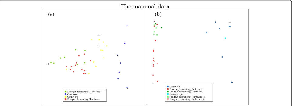
values. We choose the number of types for the mammal data as nine and apply unsupervised NMF on the data. A snapshot of the projected data on a plane is shown on the left panel of Fig. 1. From the plot, we can see that the car-nivores can be totally separated from others and the other three types are mostly separated with a few overlapping points. The dimension of the data is reduced from 1239 to 9 in this analysis.
Supervised NMF results for mammal data
We first apply supervised NMF on the whole mammal dataset. The supervised NMF did not improve the classi-fication significantly from the unsupervised NMF in this case. This is possibly because the metagenomic composi-tion of omnivores is a mixture of that of herbivores and carnivores. In order to find the most important discrimi-nant features between herbivores and carnivores, we apply supervised NMF only on the carnivores and herbivores from the mammal dataset [27]. So the data we use here contain metagenomic sequencing of fecal samples from 28 mammals: 7 carnivores and 21 herbivores. As the number of observations is small, we perform a sevenfold cross-validation on the whole data. Each time, we use six folds as training data and the remaining observations as test data. We find two types that suitably describe both classes. Then, we calculate two types on each class using the train-ing data and combine them to get the type matrixT. Fixing the type matrix, we obtain the weight matrices for the training cases and test cases by the non-negative Poisson regression method detailed in the appendix. We fit a logis-tic regression using the training data weight matrices and perform a prediction on the test data.
The projections of both training and test data in one fold of the sevenfold cross-validation, relative to the posi-tions of four types calculated from the training data, are plotted in the right panel of Fig. 1. It shows that both training carnivores and test carnivores could be well sepa-rated from herbivores. Also, from the plot, we can see that although we did not supervise the distinction between the two types of herbivores, there is some reasonable degree of separation between these two classes.
Both the training and test errors are 0 in each fold of the sevenfold cross-validation data split. The prediction errors are all 0 meaning our algorithm could separate the two classes of mammals perfectly. The huge number of variables in the original data could be reduced to four features (two for each class), which means the classes of mammals can be easily determined by four features.
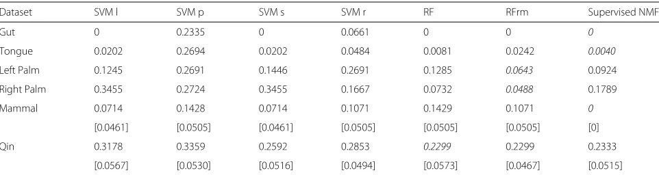
To compare the supervised NMF with support vector machine and random forest, we choose the best tun-ing parameters for SVM by the same sevenfold cross-validation as in supervised NMF. The best cost value for all kernels is 1. The best gamma value for polynomial ker-nel is 0.01, for sigmoid kerker-nel 0.001 and for radial basis kernel 0.1. We also compare with Random Forest with the sparse variables removed. (We remove the 50% of the vari-ables with lowest abundance in all samples.) The mean and standard deviation of prediction errors for models with these best tuning parameters on different folds are summarized in Table 1. The table shows that supervised NMF is among the methods which perform perfectly on the mammal data.
Interpretation of the features in the mammal data
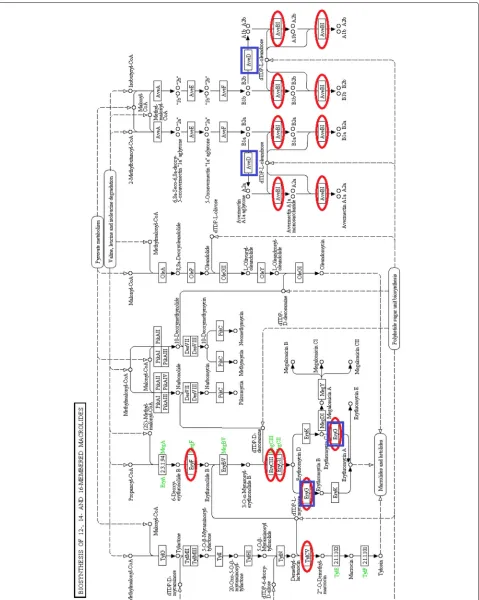
We map the features extracted separately from herbi-vores and carniherbi-vores to the metabolic pathways in KEGG. We find that most of the features from herbivores and carnivores involve the same metabolic pathways except that herbivores have more reactions in the biosynthesis of macrolides pathway, shown in Fig. 2. The most significant difference is found in one of the features of herbivores, which corresponds to the feature (cross) in the upper left corner of the right panel of Fig. 1. (This feature has been highlighted in purple on this plot.) Macrolides are a group of drugs belonging to the polyketide class of natural prod-ucts. Macrolides are not to be used on non-ruminant herbivores: they rapidly produce a reaction causing fatal digestive disturbance [31]. This explains the results that
8 out of 10 herbivores which have highest weight on this feature are non-ruminants. These correspond to the 8 hindgut-fermenting herbivores (green) in Fig. 1b. This shows that the inferred differences in the microbial com-munities of mammals relate well to the known different phenotypes for different mammals.
The moving picture data
The moving picture data [4] is the most detailed investiga-tion of temporal microbiome variainvestiga-tion to date. It consists of a long-term sampling series from two human individ-uals at four body sites: gut, tongue, right and left palm. Person 2 was measured for a longer time than person 1 (336–373 samples from each body site for Person 2 over a period of 443 days, compared to 131–135 sam-ples from each site for Person 1 over a period of 186 days). The total number of variables (different OTUs) across all samples was more than 15,000. After remov-ing all 0’s, the total number of different OTUs for the gut data is around 3000, for the tongue data is around 2000, for the left palm data and right palm data are around 13,000. In spite of this extensive sampling, no temporal core microbiome was detected, with only a small subset of OTUs reoccurring at the same body site across all time points [4].
Unsupervised NMF results for gut data in the moving picture data
First, we apply NMF to the gut data. The gut data consists of 131 observations from person 1 and 336 observations from person 2. We find the number of types is 6 based on the plot of log-likelihood values versus number of types. And we see that the data from two individuals can be well separated—see the left panel of Fig. 3. It can be seen that the four types seemed to be used to mainly describe individual 2 and two types are mainly related to individ-ual 1. It also shows that the observations for individindivid-ual 2
Table 1Comparison of test errors for support vector machine with linear kernel (SVM l), with polynomial kernel (SVM p), with sigmoid kernel (SVM s), with radial basis kernel (SVM r), RandomForest (RF), RandomForest with sparse variables removed (RFrm) and Supervised NMF
Dataset SVM l SVM p SVM s SVM r RF RFrm Supervised NMF
Gut 0 0.2335 0 0.0661 0 0 0
Tongue 0.0202 0.2694 0.0202 0.0484 0.0081 0.0242 0.0040
Left Palm 0.1245 0.2691 0.1446 0.2691 0.1285 0.0643 0.0924
Right Palm 0.3455 0.2724 0.3455 0.1667 0.0732 0.0488 0.1789
Mammal 0.0714 0.1428 0.0714 0.1071 0.1429 0.1071 0
[0.0461] [0.0505] [0.0461] [0.0505] [0.0505] [0.0505] [0]
Qin 0.3178 0.3359 0.2592 0.2853 0.2299 0.2299 0.2333
[0.0567] [0.0530] [0.0516] [0.0494] [0.0573] [0.0467] [0.0515]
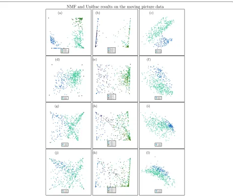
Fig. 3Top row shows results from the gut dataset (with 6 types/coordinates used for the unsupervised methods); second row shows results from the tongue dataset (with 9 types used for the unsupervised methods); third row shows results from the left palm (with 6 types/coordinates); fourth row shows results from the right palm (with 6 types/coordinates). Blue points are from person 1; green points are from person 2. Left: unsupervised NMF; middle: supervised NMF on both training and testing data— darker blue and green points are testing data; right: UniFrac.aGut NMF.bGut supervised NMF.cGut UniFrac.dTongue NMF.eTongue supervised NMF.fTongue UniFrac.gL. Palm NMF.hL. Palm supervised NMF.iL. Palm UniFrac.jR. Palm NMF.kR. Palm supervised NMF.lR. Palm UniFrac
are separated into two groups, the reason for which will become clear later in this paper.
Supervised NMF results for gut data in the moving picture data
As the gut data is time based, we choose the first 70 time points’ observations out of 131 observations of person 1 and the first 170 time points out of 336 observations of person 2 as training data. If the system changes slowly, we might expect samples from the same individual sepa-rated by only a short time might be more closely related. By choosing this separation into training and test data, we minimize the correlation between training and test
data, ensuring that we only test the method’s ability to pick up long-term microbial signatures of each individ-ual. A 10-fold cross-validation with the training data split into 10 folds sequentially over time is applied for choos-ing the number of types and we find two types for each person is the best according to our method. This is an easy classification problem: based on two types for person 1, all deviance values for person 2 are much larger than the deviance values from person 1. A total separation is almost achieved for each fold of the cross-validation for
any value of k (k ≥ 2). This is the same based on two
training W matrix and perform a prediction on the test data. The results are shown in the right panel of Fig. 3 and the prediction error is 0 for the test data.
We see that both training and test data are almost per-fectly separated between the two individuals which means the distinguishing features of the gut data are included in a matrix consisting of four features. These four fea-tures contain sufficient information for classification and will be examined in detail in the interpretation section together with the features computed from the tongue data from these two individuals, because some interesting con-nections between the tongue data features and gut data features can be detected within individual 2.
Unsupervised NMF results for tongue data in the moving picture data
Next, we apply NMF to the tongue data. For the tongue data, there are 135 observations from person 1 and 373 observations from person 2.
It is not obvious what the appropriate value for the number of types should be by looking at the plot of log-likelihood versus number of types. We try NMF on nine types and ten types. Neither achieves good separation
between samples from the two individuals. ASimplePlot
for unsupervised NMF for nine types is shown Fig. 3d as an example. Here, we see that samples from the two individuals are somewhat separated, but there is a lot of mixing: we cannot achieve a great classification from these features.
Although standard NMF works for the animal dataset and the gut dataset, it does not perform as well on the tongue dataset. The reason is that with unsupervised methods, the signal that is identified is not always the sig-nal we are interested in. Using supervised NMF, we will be able to identify the different features for different classes. This allows us to more easily distinguish samples from different classes.
Supervised NMF results for tongue data in the moving picture data
For the tongue data, as above, we choose the first 70 time points’ observations out of 135 observations of person 1 and the first 190 time points out of 373 observations of person 2 as training data. The remaining data are test data. We split the training data over time and perform a 10-fold cross-validation on the training data to find the number of types for both individuals. Our method shows that two types are appropriate for person 1, but is not so clear for person 2 (possibly suggesting nine types). Fixing two types for person 1, and comparing cross-validated error, we choose three types for person 2. This results in a test error of 0.04.
For illustration purposes, we show the SimplePlot of
both training and test data based on two types for person 1
and three types for person 2 in Fig. 3f. Through these five features, most of the observations in tongue data could be correctly classified according to which individual they come from.
Unsupervised NMF results for left palm data in the moving picture data
For the left palm data, there are 134 observations from person 1 and 365 observations from person 2. We try NMF for several different numbers of types on the left palm data. None of them achieve good separations
between samples from the two individuals. ASimplePlot
for unsupervised NMF for six types is shown in Fig. 3g as an example. Here, we see that samples from the two individuals are somewhat separated with a considerable amount of mixing.
Standard NMF does not perform well on the left palm dataset. Using supervised NMF allows us to more easily distinguish samples from different classes.
Supervised NMF results for left palm data in the moving picture data
For the left palm data, we choose the first 67 time points’ observations out of 134 observations of person 1 and the first 183 time points out of 365 observations of person 2 as training data. The remaining data are test data. Using the same procedure as for the tongue data, we find two types for person 1 and three types for person 2 can best separate the two individuals.
We show theSimplePlotof both training and test data
based on two types for person 1 and three types for person 2 in Fig. 3h. Most of the observations in left palm data could be correctly classified with a test error of 0.092.
Unsupervised NMF results for right palm data in the moving picture data
For the right palm data, there are 134 observations from person 1 and 359 observations from person 2. Similar to the results for the left palm, there is not a good separation
between samples from the two individuals. ASimplePlot
for unsupervised NMF for six types is shown in Fig. 3j as an example. Here, we see that most samples from the two individuals cannot be separated using these features.
Supervised NMF results for right palm data in the moving picture data
For supervised NMF on right palm data, we choose the first 67 time points from person 1 and the first 180 time points from person 2 as training data. The remaining data are test data. We find two types for each person can best separate the two individuals.
We show theSimplePlotof both training and test data
classified according to which individual they come from with a test error of 0.179.
Comparisons with other methods
These datasets have also been extensively analysed by BioMiCo [14]. To enable comparison with their results, we reran our analysis with individual months as training data. (Rerunning BioMiCo with our splits into training and test data is infeasible due to its excessive running time.)
We train supervised NMF on different months and pre-dict the identity of the two individuals of all other months. The number of types used for each dataset is the same as we mentioned above. Even though a smaller number of samples are used to train the model, we still get very high-classification accuracy. The accuracy is between 98.1 and 99.8% when using the gut dataset and 85.4 and 92.9% when using the tongue dataset. This is almost the same as BioMiCo’s accuracy, between 98.6 and 99.3% for the gut dataset and between 85 and 93% for the tongue dataset. However, we also get very high accuracy when using the palm data, between 88.9 and 93% when using left palm dataset and between 77.8 and 83% when using right palm dataset. This is significantly higher than BioMiCo’s results (40 to 75%). Palm data are more challenging because human palms are exposed to the external environment. The comparison with BioMiCo concludes that the super-vised NMF is not only efficient in terms of computation but also better at finding discriminant features of individ-uals even with very noisy data.
We also compared supervised NMF with support vector machine, random forest and random forest with sparse variables removed on this moving picture data. We split each body part’s data in the same way as that in supervised NMF. A 10-fold cross-validation is applied to the training part to calculate the best tuning parameters. Models with the best tuning parameters then are trained on the whole training data and used to predict the test data. The results are summarized in Table 1. The comparison for moving picture data shows that supervised NMF gives comparable or better classification results than other methods except for the left and right palm dataset. For these datasets, ran-dom forest on the most abundant OTUs performed better than NMF. For the left palm data set, random forest on all variables performed better than NMF.
UniFrac is a widely used unsupervised method. To compare the separation of two individuals, we project the samples on principal coordinates of the unweighted UniFrac distance matrix (based on rarefied samples) in the right-hand column of Fig. 3 with the numbers of the principle coordinates equal to the numbers of types
we have used for each case, presented using
Simple-Plot. We can see a clear separation of the two indi-viduals from the gut dataset. Plots of tongue data and palm data show separations to some degree, but not as
clear as in our unsupervised NMF plots (left panels in Fig. 3). This shows NMF is an alternative and possibly more useful data exploratory method for such data. In addition, NMF has a natural interpretation in terms of mixtures of communities, but the results from UniFrac are hard to interpret, as they cannot show what causes the grouping effects or where the differences in microbime composition lie.
Interpretation of the results
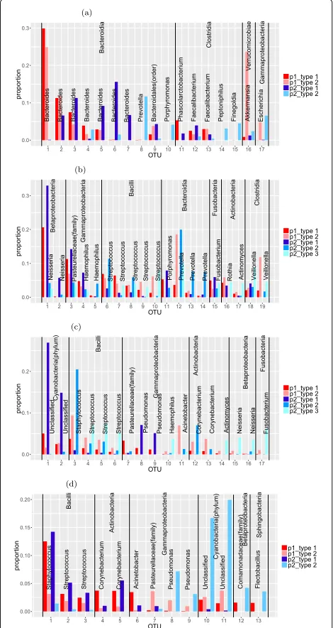
To examine the main aspects of the features identified, we plot the relative abundance of OTUs for different features in Fig. 4. The feature vectors are of the same dimension as the original observations. A natural side effect of NMF is that the resulting feature vectors are usually sparse. The feature vectors consist of non-negative elements with each vector sum equal to 1. The non-zero values can be inter-preted as the percentages of the OTU composition in a particular feature. To get a better illustration, we use a cut-off of 3% for each feature vector in Fig. 4. That is, only those OTUs with above 3% composition in at least one feature are included in the plot.
Figure 4a shows the main OTUs for the gut data. We find only 17 out of more than 3000 OTUs are larger than the cut-off of 3%. Among these major OTUs, the two fea-tures within each individual bear some similarities. But the features between two different individuals are quite different. This is reflected by the fact that several of the most common OTUs in individual 1’s features are not present in individual 2’s features and vice versa. Since each individual’s data can be best represented by his/her own two features and their two features are largely dif-ferent, this partially explains why the classification of two individuals based on the gut data is an easy problem.
Figure 4b shows the main OTUs for the tongue data. There are only around 20 OTUs in tongue features above the cut-off of 3%. Again the type matrix of the tongue data is highly sparse. Unlike the features of the gut data, the features of the tongue data for these two individuals are more similar. By looking at the compositions of the most dominant OTUs in each feature, we can easily see simi-larities between person 1’s type 1 and person 2’s type 1. Also person 1’s type 2 is similar to person 2’s type 2 for OTUs in the classes Fusobacteria and Gammaproteobac-teria and similar to person 2’s type 3 for OTUs in the class Bacilli. This suggests that there are similar variation pat-terns between the two individuals, with the same groups of OTUs increasing or decreasing together. Naturally, the classification for the tongue data is a harder problem.
Fig. 4Outstanding OTUs in features of moving picture data: The light and dark red bars are two features from person 1 and the blue bars are features from person 2. The OTUs from the same class are in the same block which is labeled by their class name and the bars are labeled by the genus of the OTUs. The two unlabeled bars in left palm data are the same OTUs with these unlabeled bars in the right palm plots. They are two different unclassified classes in Cyanobacteria phylum.aOutstanding OTUs in features of gut data.bOutstanding OTUs in features of tongue data.cOutstanding OTUs in features of left palm data.dOutstanding OTUs in features of right palm data
with some variations in their values. The features within individual 2 show a different pattern with each OTU mainly represented by one of the three features. Left palm features within each individual are quite differ-ent because the palm’s microbial environmdiffer-ent is more
variable. Features between individuals are also quite dif-ferent for most of these major OTUs. Several OTUs in individual 2’s features are not present in individual 1’s features. This may explain why the left palm data can achieve high classification accuracy but lower than the gut data.
Figure 4d shows the main OTUs for the right palm data. There are only 13 OTUs in right palm features above the cut-off of 3%. The patterns of features within each individ-ual are similar to their left palm data. But features between individuals are more similar except differences in the two unlabeled OTUs. This explains the difficulty in separat-ing two individuals from the right palm data. We also find major OTUs in the right palm features are nearly all present in the left palm features. We do not find the same situation in gut and tongue features. This may be because an individual’s left and right hands are usually exposed to the same environment. It could also be caused by contact between the two hands.
In many of the examples, NMF can act like a vari-able selection method—identifying individual reactions or OTUs which show different abundances in the two groups of samples. However, in the moving picture tongue dataset, we do not obtain such good classification by look-ing at individual OTUs. Instead, we look more deeply at the community structure identified by NMF. By examin-ing community-level differences, we were able to classify the individuals with a very high degree of accuracy. We now look in more detail at the communities involved, in an attempt to understand why unsupervised NMF was less effective in this case, and why supervised NMF was able to resolve this problem. This also demonstrates more of the range of interpretability offered by NMF. In addi-tion to highlighting individual OTUs or reacaddi-tions that differ between the two classes, it is able to isolate bacte-rial subcommunities from which the microbiome is built up and offer insights into the different structures of these communities.
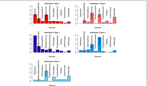
Figure 5 shows the profiles of the types extracted from the two individuals, with graphs of abundance of each genus in that type. For individual 1, we see that type 1
con-tains higher abundances ofNeisseria,Haemophilus,
Por-phyromonas, Fusobacterium and the unclassified genus from the Pasteurellaceae family, while type 2 includes
higher abundance of Streptococcus, Prevotella, Rothia,
ActinomycesandVeillonella. This may well be associated
with the action ofPorphyromonas. One species,
Porphy-romonas gingivalis, has been shown in [32] to manipulate the host immune system, allowing pathogens to colonise
the community. While the OTU from the genus
Fig. 5Major genera for tongue feature matrix. The light and dark red bars are two features from individual 1 and the blue bars are features from individual 2. Each bar is labeled by the name of the genus or family
closely related to known pathogens. When we look at the features for individual 2, we see a similar picture, with types representing varying levels ofPorphyromonas.
Again, we see with increased Porphyromonas, we have
an increase in Neisseria, Haemophilus, Fusobacterium,
and the unclassified genus of the Pasteurellaceae fam-ily, and a corresponding decrease inStreptococcus, Pre-votella,ActinobacteriaandVeillonella. Type 2 may show that the effect ofPorphyromonasis non-linear with Pre-votellaactually increasing in abundance with low levels of Porphyromonas.
We also examine the types in the absence of
Porphy-romonas(type 2 for individual 1 and type 3 for individ-ual 2). For both individindivid-uals, we see that these types are
dominated by Streptococcus, Prevotella and Veillonella.
However, Fig. 4b shows the differences between these
types. We see that individual 2 has moreActinomycesand
a different distribution between OTUs within the genus Veillonella. Similarly, there are subtle differences between
the types with high abundance ofPorphyromonas(type 1
for both individuals). Individual 1’s type 1 has higher
lev-els of Streptococcus than individual 2’s. This might be
partially explained by the use of three types to model individual 2, allowing separate types to model both high
and low levels of Streptococcus in cases with high
lev-els of Porphyromonas. However, in Fig. 4b, we see the
presence of higher abundance of a second OTU from the genusNeisseriain individual 2’s type 1. This cannot be explained by the different numbers of types used to analyse the two individuals. Supervised NMF is able to identify these subtle differences and use them to identify the individuals, even in situations where the large-scale community structure varies a lot between samples within each individual.
We also consider the idea that the types correspond to communities of microbes. When we look at the type
withoutPorphyromonas, we can see the makings of a
com-munity structure, with a number of microbes (such as Pre-votella,StreptococcusandActinobacteria) that metabolise glucose into pyruvate, which is later metabolised into
lactate, and other microbes such as Veillonella which
metabolise lactate.
Temporal dynamics
Fig. 6Gut and tongue weight matrix time series plot for person two. The top plot shows the gut weight matrix on the second type (red line) and third type (blue line) from NMF with 3 types. The bottom plot shows the tongue weights on the first type (red line) and the third type (blue line) from NMF for tongue data with 4 types
data, this shift is not very clear when we use only three types. However, with four types, we can identify a more apparent shift in their weight matrix time series plots. For this data one more feature can bring out more details in the variation of the data. In the lower panel of Fig. 6, the weight matrix time series plots for the tongue data relative to these two features show that type 1 is consis-tently more represented than type 3 in the early part of the study although not always dominant due to the effects of types 2 and 4; type 3 is more represented than type 1 after the changing point (highlighted on the plot). The shift occurs first in the tongue weight matrix and then can be detected about 4 days later in the gut weight matrix. This suggests that some significant change has taken place in person 2’s system at around this time and that the change has influenced both the gut and the tongue microbiomes.
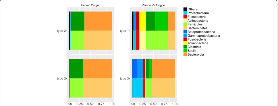
In order to compare the changes which we have iden-tified as taking place in these microbiomes, the distribu-tions of different phyla and classes of OTUs in each feature are presented in Fig. 7. The top features in this plot are the ones that are more represented in the earlier part of the data (i.e. type 2 for the gut data, and type 1 for the tongue data). The bottom features in this plot are those that are more represented in the later part of the data.
Figure 7 shows a similar shift of composition between the two features for both gut and tongue. In both cases, the type which was more represented in the earlier part of the study has a lower proportion of Bacteroidia and a higher proportion of Clostridia. The proportion of Bacteroidia increases and the proportion of Clostridia decreases for both representative features of gut and tongue data in the later part of the study. The consistency of these changes
between the two datasets gives further support to our conjecture that this represents a systematic change at this time. The differences between the types are more pronounced in the tongue data. This could be because the tongue is more exposed to external influences, so its microbiome may be more variable. It might also be because we were using four types to model the tongue data and only three for the gut data. Fitting more types gives the types more room to spread out, allowing for more extreme types and amplifying the differences between the fitted types.
We see that the changes shown in Fig. 7 are consistent with the earlier interpretation of the types in Fig. 5. We used four types here to model the microbiome, but we can see in Fig. 7 that the dominant type after the tran-sition includes much higher abundances of Bacteroidetes
(includingPorphyromonasandPrevotella, which has been
associated with Periodontal disease [33]) and
Proteobac-teria (including Neisseria and Haemophilus) and lower
levels of Firmicutes (including Streptococcus and
Veil-lonella) and Actinobacteria (includingRothiaand Actino-myces). Note that the types in Fig. 5 are fitted from the training data, which is entirely before the state change in person 2.
Having identified the state change using NMF, we ask whether NMF was a necessary tool for identifying the change. First, we compare a naive examination of the com-position of the microbiome by class. Figure 8 shows the smoothed proportion of each class over time in person 2’s gut and tongue microbiomes. We see that there are no clear changes in composition at this level, indicating that this is not an obvious change to identify.
For comparison, we also use UniFrac and PCoA for per-son 2’s gut and tongue data. We see that the first three principal coordinates for the gut data and the first four coordinates for the tongue data do not reveal this change. It is only when we examine the 4th principle coordinate for the gut data and the 5th principle coordinate for the
tongue that we are able to detect the changes. The dif-ficulty of finding this explains why this pattern was not found in the many previously published analyses of these data. This is made more difficult by the common practice of examining only the first three principal coordinates. It is possible to find the pattern using UniFrac, if one knows what to look for, but NMF certainly makes the pattern much easier to find.
The Qin data
The Qin dataset [28] contains human gut metagenome samples extracted from 99 healthy people and 25 IBD patients. The data include 2804 different reactions.
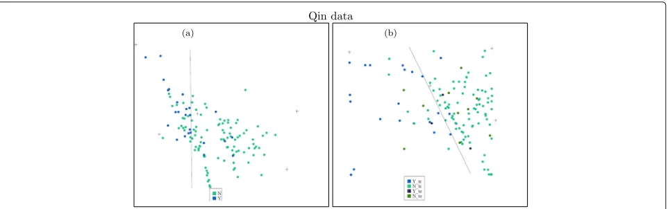
Unsupervised NMF results for Qin data
We choose the number of types for the Qin data as six and apply unsupervised NMF on the data. A projection of the data onto a plane is shown on the left panel of Fig. 9. From the plot, we can see that about 19 of the IBD patients can be separated from healthy people. The separation is similar to the results of BiomeNet [15]. The plot shows that two of these features are more related to IBD patients and the other four more related to healthy people. This is consistent with what we find using supervised NMF.
Supervised NMF results for Qin data
The sample size of patients is much smaller than the sam-ple size of healthy peosam-ple. So we perform a classification giving the patients a weight of 4 to balance the class sizes. (For supervised NMF, these weights do not affect the fitted matricesTandW, only the classifier applied to the weight matrixW.) This means that the classifier that assigns all samples to one class will have an accuracy of about 50%. We perform a 10-fold cross-validation on the whole data. Each time, we use nine folds as training data and the remaining observations as test data.
We find two types are enough for patients and four types for healthy people. We perform supervised NMF
Fig. 9Left: unsupervised NMF based on 6 types. The blue points are from IBD patients and the green ones are from healthy people. Right: supervised NMF on both training and test data. The blue points are training data from patients, and green points are training data from healthy people; the dark blue points are test data from patients, and the dark green points are test data from healthy people.aUnsupervised NMF.bSupervised NMF
and fit a logistic regression using the training data weight matrices (with patients given weights of 4) and perform a prediction on the test data. The average of the weighted prediction error over the 10 folds is 0.233 with a standard error of 0.0487.
The projections of both training and test data in one fold of the 10-fold cross-validation are plotted in the right panel of Fig. 9. It shows a quite good separa-tion between these two groups. The classificasepara-tion is not perfect, but is an improvement upon previous methods, such as BiomeNet [15].
The comparisons with support vector machine and random forest methods are summarized in Table 1. The dataset is split to the same 10 folds as supervised NMF. The best parameters are tuned by a 10-fold cross-validation on the whole dataset. The best cost parameter in SVM function is 3 for radial basis kernel and 1 for other three kernels. The best gamma parameter is 10−4for radial basis kernel, 0.1 for polynomial kernel and 0.001 for sigmoid kernel. No method performed significantly better than supervised NMF.
Interpretation of the results
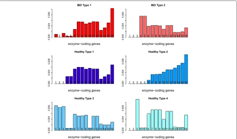
The six type vectors are highly sparse with each vec-tor sum equal to 1. We use a cut-off of 0.5% for each type to find the distribution of each type over the major reaction groups. Here, each reaction group includes the different reactions that correspond to the same enzyme-coding gene; thus, each category can also be understood as corresponding to one enzyme-coding gene. The type dis-tribution over 17 enzyme-coding genes or reaction groups is shown in Fig. 10. We can observe that theIBD Type 2is quite different from other types, with large abundance on the fourth and fifth enzyme-coding genes and that both IBD types have weight zero on the second enzyme-coding gene. Each individual’s metagenome profile is expressed
as a linear combination of these six types; the weight dis-tribution over each type is shown in Fig. 11, where the top part of each bar presents the distribution of the weights for healthy individuals for the corresponding type, and the bottom part of each bar is for the weight distribution of IBD patients with each patient counted as four times to make the results comparable to the healthy individuals. From Fig. 11, we can see the IBD patients mainly have
non-zero weights onIBD Type1,IBD Type2,Healthy Type
1andHealthy Type 2, and healthy individuals mainly have
non-zero weights onHealthy Type 1,Healthy Type 2and
Healthy Type 4. It seems that the IBD Type 2 typically represents a group of IBD patients andHealthy Type 2 rep-resents a group of healthy individuals with these two types distributed very differently over the enzyme-coding genes shown in Fig. 10.
According to Fig. 10, the first three reaction groups con-tribute more to healthy types and the fourth and fifth reaction groups contribute more to IBD patients (mainly to IBD Type 2). Reactions in the first group are all in macrolide biosynthesis. Macrolides are protein synthesis inhibitors and can be used as an antibiotics treatment of inflammatory diseases including inflammatory bowel disease [34–36]. The second reaction group is involved in polycyclic aromatic hydrocarbon degradation and the third group is in carotenoid biosynthesis. Polycyclic aro-matic hydrocarbons (PAHs) are one family of ubiquitous environmental toxicants. This family has contributed sig-nificantly to the development of colorectal cancer (CRC), a disease highly linked to IBD [37]. Carotenoids can enhance the human immune system’s effectiveness [38]. As IBD is a kind of autoimmune disease, this could explain why these two compounds are lower in IBD patients’
fea-tures. The fourth group in IBD Type 2 is involved in
Fig. 10Qin data: the distribution of each type over major enzyme-coding genes:IBD Type 2typically represents a group of IBD patients andHealthy Type 2represents a group of healthy individuals with these two types distributed very differently over the enzyme-coding genes
and mannose metabolism, glycolysis and gluconeogene-sis and additional pathways. These are concordant with BiomeNet’s findings in subnetworks 38, 64 and 73. Com-paring our reaction groups with the three subnetworks, we notice that reaction group 4 can be found in subnet-work 64 and group 5 has some overlaps with subnetsubnet-work 38 and subnetwork 73. These three subnetworks were dis-covered to have a larger contribution to IBD samples than healthy ones.
Simulations
Simulation based on NMF
We perform simulations in this section to evaluate the performance of our proposed method with regard to the number of types selected and prediction accuracy. We use types estimated from the Qin data [28] to do the simulation. We simulate data according to our proposed model. The data follows a Poisson distribution with mean
(TW)ij. To generate these data, we first generate the
meanTW.
The mean is a linear combination of different features
(different columns of T). We fix T to be the features
obtained by applying NMF to the two classes in the Qin dataset [28].
We generate the W matrix by generating each entry
from a uniform distribution on [0, 1] , then normalizing
the column vectors so that the column sums ofW are
equal to the column sums of the IBD data.
The productTW gives us the mean, and we add four
levels of noise to the productTW. The noise is normally
distributed with mean 0 and four different standard devi-ations, to study the effects of different signal-noise ratios (SNR).
SNR= +∞:sd0=0
SNR=4 :sd1=sd(T)/4
SNR=2 :sd2=sd(T)/2
SNR=1 :sd3=sd(T)
Here, the sd(T) is a vector of standard deviations for each row ofT. This is a vector of length p (the number of genes or OTUs) which measures the variability for each gene or OTU across different features inT.
The column ofTW plus the noise is the Poisson mean
we use in the simulation. Each element ofXis generated
following an independent Poisson distribution with the mean given by the mean matrix described above.
Fig. 11The weights distribution over each type for heathy individuals (top for each bar) and IBD patients (bottom for each bar): the IBD patients mainly have non-zero weights onIBD Type1,IBD Type2,Healthy Type 1andHealthy Type 2, and healthy individuals mainly have non-zero weights on
Healthy Type 1,Healthy Type 2andHealthy Type 4
we simulate 25 replicates. In each replicate, we simulate 200 observations for each class. Then, we separate the data into two parts: the first 200 observations (100 from each class) as the training data and the other 200 as the test data.
We choose the number of types from the training data using a 10-fold cross-validation. After the number of types is chosen, we perform a prediction on the test data using the trained logistic regression model on the training data based on the chosen number of types for each simulated data set.
The NMF, RF and SVM prediction errors are shown in Tables 2, 3 and 4 respectively for different noise levels. We find when the true numbers of types get larger, the NMF prediction errors tend to increase but the RF pre-diction errors tend to decrease. That may be because we have more accurately estimated the number of types in the cases when the true numbers of types are small. But overall, the prediction errors are quite small for all cases which means our supervised NMF method works well in prediction. NMF performs better in prediction than RF when number of types is small and better than SVM in all scenarios.
Table 5 summarizes the results of the number of types chosen. It shows that the algorithm tends to output slightly larger values than the true number of types in
most scenarios, but the true numbers of types mostly are within one standard deviation of the mean of the chosen number of types. Note also, the number of types are cho-sen only by performing the Wilcoxon Rank-Sum test for each class (see the appendix), the results are not modified
Table 2NMF mean prediction test errors for 25 data sets with the standard errors for the mean prediction errors (mean/SE)
SNR class 1\class 2 2 types 5 types 10 types
+∞ 3 types 0.0002/0.001 0.004/0.0066 0.0104/0.0126 4 0.0002/0.001 0.005/0.0085 0.0092/0.0102
2 0.0002/0.001 0.0048/0.0071 0.0102/0.0104
1 0.0002/0.001 0.0022/0.0041 0.0084/0.0079
+∞ 6 types 0.0012/0.0036 0.0054/0.0071 0.0082/0.0089 4 0.0012/0.0030 0.0052/0.0076 0.0154/0.0114
2 0.001/0.0029 0.0056/0.0082 0.0058/0.0067
1 0.0014/0.0037 0.0058/0.0081 0.0126/0.0107
+∞ 9 types 0.0106/0.0132 0.0068/0.0084 0.0108/0.0126 4 0.0088/0.0102 0.0066/0.0100 0.0132/0.0100
2 0.0078/0.0101 0.0072/0.1011 0.0128/0.011
1 0.0046/0.0058 0.0062/0.0092 0.0124/0.0089
Table 3RF mean prediction test errors for 25 data sets with the standard errors for the mean prediction errors (mean/SE)
SNR class 1\class 2 2 types 5 types 10 types
+∞ 3 types 0.0024/0.001 0.0012/0.0007 0.0012/0.0005 4 0.0014/0.0004 0.0002/0.0002 0.0012/0.0005
2 0.0016/0.0006 0.0016/0.0006 0.0006/0.0003
1 0.0018/0.0006 0.0008/0.0004 0.001/0.0005
+∞ 6 types 0.0022/0.0007 0.0026/0.0009 0.0008/0.0005 4 0.002/0.0007 0.0018/0.0008 0.001/0.0006
2 0.002/0.0008 0.0014/0.0005 0.001/0.0005
1 0.002/0.0008 0.0024/0.0008 0.0006/0.0004
+∞ 9 types 0.0028/0.001 0.0014/0.0007 0.001/0.0006 4 0.0022/0.001 0.0014/0.0006 0.0014/0.0007
2 0.0022/0.0009 0.001/0.0005 0.0008/0.0004
1 0.0022/0.0007 0.0008/0.0004 0.001/0.0005
through optimizing the classification results based on combined types.
Table 5 also shows that in most replicates, when the noise level becomes higher, the difference between the mean and the true number of types will increase. Never-theless, these results demonstrate that our method is quite effective in finding the appropriate number of types.
Further simulation results (not shown in this paper) have shown that when we apply NMF with the true num-ber of types on the simulated data, the features computed from the data can match very closely with the true features that were used to generate the data. Applying NMF with the wrong number of features can recover a space with the true features embedded in it. The study of consistency of
Table 4SVM mean prediction test errors for 25 data sets with the standard errors for the mean prediction errors (mean/SE)
SNR class 1\class 2 2 types 5 types 10 types
+∞ 3 types 0.1462/0.0173 0.13/0.0167 0.1276/0.0156 4 0.1356/0.0176 0.1784/0.0169 0.1616/0.0153
2 0.1356/0.0176 0.1784/0.0168 0.146/0.0124
1 0.1356/0.0176 0.185/0.0151 0.146/0.0125
+∞ 6 types 0.1794/0.018 0.1214/0.0146 0.162/0.0154 4 0.1774/0.0191 0.1626/0.0154 0.1738/0.0164
2 0.1772/0.0191 0.1498/0.0147 0.159/0.0172
1 0.1392/0.0173 0.1632/0.0154 0.1248/0.0151
+∞ 9 types 0.1344/0.0193 0.1656/0.0179 0.174/0.0177 4 0.121/0.0158 0.1558/0.0166 0.1846/0.0162
2 0.121/0.0158 0.1552/0.0181 0.1824/0.0177
1 0.121/0.0159 0.1652/0.0198 0.1794/0.0178
Table 5Simulation summary of the estimated numbers of types
SNR 2 5 10
Mean sd Mean sd Mean sd
+∞ 3 2/3.4 0/1.0 5/3.1 0.3/0.3 8.9/3.5 1.9/1.3 4 2/3.8 0/1.5 5/3.3 0.3/1.2 8.9/3.7 2.2/2.0
2 2/3.7 0/1.4 5/3.1 0.3/0.3 8.9/3.7 2.2/2.0
1 2/3.6 0/1.4 5.1/3.0 0.5/0.2 8.5/3.8 1.9/2.0
+∞ 6 2/6.4 0/0.8 5/6.4 0.5/0.7 9.8/6.6 1.2/1.2 4 2/6.4 0/0.6 5.2/6.6 0.8/0.9 9.5/6.4 1.3/0.6
2 2/6.4 0/0.6 5.2/6.6 0.5/0.8 9.4/6.3 1.5/0.5
1 2/6.3 0/0.6 5.0/6.6 0.5/0.8 9.4/6.2 1.1/0.5
+∞ 9 2.4/8.4 1.5/1.5 5.1/8.9 1.7/0.8 8.7/9.2 1.8/0.8 4 2/8.2 0/1.7 5/9.8 0.4/1.1 8.8/9.2 1.8/0.6
2 2.4/9.1 1.5/0.7 7.0/9.3 1.5/0.8 11.0/10.9 1.2/1.4
1 2.5/9.0 1.1/1.1 6.9/8.7 1.8/0.9 9.7/10.8 1.7/1.8
For example, the first entry 2/3.4 means when the true number of types is 2 for class 1, 3 for class 2 andSNR= +∞, the mean numbers of types our method chooses are 2 for class 1 and 3.4 for class 2
the NMF method is not a trivial topic and deserves further research.
Simulation with outliers
We designed this simulation to measure how our method performs when the data contain outliers. We perform this simulation based on data generated in the last section. We use the generated data of scenarios 2&3 types, 5&6
types and 10&9 types, with SNR = 1. We
gener-ate outliers by mislabeling the class of observations in the training data. We run simulations with 5, 10 and 20% of observations in the training data mislabeled. We used the same procedure as in the previous section to calculate the prediction errors. The results in Table 6 show that while RF is more robust in this simulation, NMF still predicts fairly well when there are outliers in the data.
Simulation with zero inflated weight matrix