Unsupervised Evaluation and Weighted Aggregation of
Ranked Classification Predictions
Mehmet Eren Ahsen1,2 [email protected]
Robert M Vogel2,3 [email protected]
Gustavo A Stolovitzky2,3
1University of Illinois at Urbana-Champaign
Department of Business Administration, 1206 S 6th St, Champaign, IL 61820, USA
2Icahn School of Medicine at Mount Sinai
Department of Genetics and Genomic Sciences One Gustave Levy Place, Box 1498
New York, NY , USA
3IBM T.J. Watson Research Center
1101 Kitchawan Road, Route 134, Yorktown Heights, N.Y., 10598, USA.
Editor:Samy Bengio
Abstract
Ensemble methods that aggregate predictions from a set of diverse base learners consis-tently outperform individual classifiers. Many such popular strategies have been developed in a supervised setting, where the sample labels have been provided to the ensemble algo-rithm. However, with the rising interest in unsupervised algorithms for machine learning and growing amounts of uncurated data, the reliance on labeled data precludes the ap-plication of ensemble algorithms to many real world problems. To this end we develop a new theoretical framework for ensemble learning, the Strategy for Unsupervised Multiple Method Aggregation (SUMMA), that estimates the performances of base classifiers and uses these estimates to form an ensemble classifier. SUMMA also generates an ensemble ranking of samples based on the confidence score it assigns to each sample. We illustrate the performance of SUMMA using a synthetic example as well as two real world problems.
Keywords: Ensemble learning, Ensemble classifier, Unsupervised Learning, AUC, Spec-tral Decomposition
1. Introduction
Algorithmic solutions to typical machine learning problems are quickly increasing in number and complexity. However, no algorithm performs best under every circumstance: there is no one-size-fits-all solution in machine learning. A mathematical formulation of this phenomena is known as the “no free lunch” theorem (Wolpert, 1996). On the other hand, it has long been appreciated that the combination of different algorithms, both in classification and regression tasks, results in more robust solutions (Dietterich, 2002).
c
Indeed, the endeavor of combining predictions or preferences from multiple sources has been institutionalized and incorporated in our everyday decision making. For example, in democratic elections the candidate who gets the most votes wins, or in online purchases the products with better customer reviews are more likely to be chosen. In social sci-ences this collaborative decision-making process is known as the Wisdom of Crowds (WOC) (Surowiecki, 2005). In the machine learning literature, the process of combining multiple base learners is known as ensemble learning.
Ensemble algorithms can be divided into two main categories, namely supervised and unsupervised ensemble algorithms. Supervised ensemble algorithms can be further subdi-vided into two main subcategories. The first represents homogeneous ensemble algorithms that consist of training several instances of a single type of algorithm on various splits of labeled data. This subcategory of methods generates diversity by subsampling training examples (bagging) (Breiman, 1996) or assigning weights to training examples (boosting) (Freund and Schapire, 1997; Schapire, 1990) utilizes a single type of base classifier to build the ensemble classifier. Homogeneous ensembles may suffer in applications where the data is very complex, and consequently the most appropriate base classifier model is not known
a priori. The second subcategory is known as heterogeneous ensemble algorithms, where each base classifier represents a distinct algorithm. Two popular heterogeneous ensemble methods are a form of meta-learning called stacking (Wolpert, 1992) as well as the ensem-ble selection procedure proposed in (Caruana et al., 2004). Among them, stacking trains a higher-level classifier over the predictions of base classifiers, while ensemble selection uses an iterative strategy to select an optimal set of base classifiers that balances diversity and performance.
Although supervised heterogeneous ensembles often out-perform homogeneous ensem-bles (Niculescu-Mizil et al., 2009; Gashler et al., 2008), there are several limitations regard-ing their use in real life scenarios. Along with the risk of overfittregard-ing associated with the meta-training of ensemble classifiers, another very important limitation of heterogeneous supervised ensemble algorithms is that in many domains labeled data for training ensemble classifiers are scarce and, in some cases, there may not be any available at all. For such cases, unsupervised learning methods might be more appropriate. Unsupervised ensemble learning has been used successfully in diverse applications including computational biology (Marbach et al., 2012), crowdsourcing in natural language tasks (Snow et al., 2008), and business (Tsai and Hsiao, 2010). The simplest unsupervised ensemble algorithm creates an ensemble score by an unweighted average of the ranks assigned by the base classifiers to each item being classified (Marbach et al., 2012; Emerson, 2013). We will call this simple unsupervised ensemble method as the “Wisdom of Crowds” (WOC) approach (Surowiecki, 2005). The WOC approach suffers when the majority of base classifiers perform poorly. A strategy to mitigate this shortcoming would be to assign each base classifier a weight commensurate (e.g., proportional) to its performance. However, this approach may not be advisable or applicable when (1) the biases of the training sets are different from the test set, or (2) there is scarce or no prior labeled data sets to calculate performance.
al-gorithm (Dempster et al., 1977). While elegant, this solution to the unsupervised ensemble construction suffers from the known limitations of the EM algorithm for non-convex opti-mization problems. Another important limitation is the strong assumption of conditional independence which might be violated in practical settings.
In this work, we propose a new theoretical framework for unsupervised ensemble learn-ing, the Strategy for Unsupervised Multiple Method Aggregation (SUMMA). Our work is a generalization of the Spectral Meta-Learner (SML) theory developed in Parisi et al. (2014). In SML, the authors starting point is the covariance matrix of predicted binary labels of a set of base classifiers. They show that under the assumption of conditional independence of the class predictions of base classifiers given the true class labels, the off-diagonal elements of the covariance matrix are related to the balanced accuracy of each base classifier. Many popular classification algorithms such as logistic regression (Harrell, 2001), SVM (Support Vector Machines) (Cortes and Vapnik, 1995), and deep learning algorithms (Chollet, 2017) produce continuous scores that can be interpreted as a measure of the confidence assigned by the base classifier that a given item is of one of the two binary classes. By forcing base classifiers to produce binary predictions SML is not only ignoring the readily available continuous scores outputted by typical base classifiers, but it also runs into the risk of over-fitting by requiring each algorithm to define a threshold to binarize its output. In the case of SUMMA, our starting point is the covariance matrix of ranked predictions which can be created by rank ordering the continuous scores outputted by the base classifiers. We show that the off-diagonal entries of this covariance matrix are related to the Area Under the Receiver Operating Characteristics Curve (AUC) (Marzban, 2004) of the base classifiers. Under the assumption of conditional independence of the ranks assigned by base classifiers to an item given the class of the item, the SUMMA algorithm:
1. Infers the empirical performance, as measured by the AUC, of each base classifier without labeled data,
2. Uses the inferred performances of the base classifiers to generate an aggregate contin-uous score for each sample, and
3. Uses these scores to predict the binary class labels for each sample.
To exemplify our theoretical results we first apply SUMMA to a simulated dataset where our theoretical assumption of conditional independence strictly holds. We also apply SUMMA to two datasets taken from real applications where we show that SUMMA performs robustly even if the conditional independence assumption is slightly violated.
2. Problem Setup
Given a classification problem, we assume that an instance pair (X, Y) ∈ X × {0,1} is a random vector with probability density function p(x, y) and marginals PX(x) and PY(y), where the set X denotes the feature space, and without loss of generality, y = 0 denotes the negative class and y = 1 denotes the positive class. Let {gi}Mi=1 represent an ensemble of classifiers with unknown reliability, where each classifier, gi : X → R, is a mapping
gi(xk) associated with a set of N instances D={(xk)}Nk=1 ⊂ X, whose true but unknown class labels are denoted by the vector y = [y1,· · · , yN]T. We let N1 := PNi=1yi denote the number of positive instances, N0 = N −N1 denote the number of negative instances and ρ = N1/N denote the prevalence of the positive class, which we simply denote as prevalence in the text. We can interpret the output of each classifier as a measure of the relative confidence that the sample belongs to one of the classes, which, without loss of generality, will be assumed to be class 1. For example, in a Bayesian framework the output of a classifier is the posterior probability that a sample belongs to the positive class. In the case of SVM, the output is the distance to the separating hyperplane.
Recent research suggests that appropriate calibration of the classifier outputs will boost the performance of the ensemble classifier (Whalen and Pandey, 2013; Bella et al., 2013). In the current manuscript, we will use the rank transformation as a calibration tool due to its theoretical implications presented in the subsequent sections. Accordingly, let Ω = {(x1, y1),· · · ,(xN, yN) ∈ (X × {0,1})N : PNi=1yi = N1} denote the space of all N i.i.d realizations ofX × {0,1}with exactly N1 positive instances. For eachT ∈Ω and classifier
i, consider the following vector gi(T) = [gi(x1),· · · , gi(xN)]T ∈ RN. By using the
well-ordering property of the real numbers, we can mapgi(T) to a rank vectorr= [r1, ..., rN]T ∈ SN, whereSN denotes the set of all permutations of the integers{1,· · · , N}.As in the recent literature (Agarwal et al., 2005), we assume that ties, i.e. gi(xj) = gi(xk) for j 6= k, are broken uniformly at random. In this case, w.l.o.g., we assume that gi assigns ranks to tied samples according to their position in the vector gi(T). Throughout the rest of the manuscript, unless otherwise noted when we say we are given a realizationT ∈Ω, we assume that we do not observe the labels associated with each sample and only observe the feature vector xk associated with each sample. With the above notation, we let P(Ri = r|yk) denote the probability, over all realizations from Ω, that a sample of class yk ∈ {0,1} has been assigned rank r ∈ {1,· · · , N} by the classifier i. For simplicity, we will refer to this quantity asPi(r|yk) and also letP(R1 =r1k, R2 =r2k,· · ·, RM =rM k|yk) denote the joint probability of each classifier iassigning rank rik to a samplekof classyk.
3. Theory
3.1. Performance Metric
We start by defining the main performance metric that is primarily used throughout the paper.
Definition 1 The performance of the ith classifier is measured by,
∆i =E[Ri|y= 0]−E[Ri|y = 1],
where E[Ri|y = j], for j = 0,1, represents the average rank given the respective class for
the ith classifier.
∆i is defined over the set Ω and as such it may depend onN andρ. Note that a random method has ∆i=0. Intuitively, this is because random methods are those unable to rank samples according to the latent class, a consequence of the fact that for a random method
set of integers{1,2, ..., N}. On the other hand if |∆i|>0, then method iis an informative method and can discriminate rank assignments by the sample class.
We will assume that all methods i = 1, ..., M use the same convention consisting of assigning ranks to the examples predicted to be in the positive class in the lower range values of the interval 1, ..., N, and the examples predicted to be in the negative class to the upper range of the same interval. In this way, a perfect classifier gP would assign the ranks [1,2, ..., N1] to theN1 positive examples, and the ranks [N1+ 1, ..., N] to the negative examples. In this case E[RP|y = 1] = (N1 + 1)/2, E[RP|y = 0] = (N +N1 + 1)/2 and ∆P =N/2.
3.2. Conditionally Independent Classifiers
In this section we first define the conditional independence assumption which is central to our theoretical results. We call the classifiers, {g1,· · · , gM}, lth order conditionally independent, if for any L = {gi1,· · · , gil} ⊂ {g1,· · · , gM} their conditional distribution
factorizes,
P(Ri1 =ri1k, Ri2 =ri2k,· · ·, Ril =rilk|yk) =Pi1(ri1k|yk)Pi2(ri2k|yk)· · ·Pil(rilk|yk). (1)
Next we prove that under the assumption of conditionally independent classifiers, their higher-order covariance tensors have a specific form.
Theorem 2 Suppose the classifiers {g1,· · · , gM} are lth order conditionally independent
so that equation (1)holds. For any n≤l≤M, let thenth order covariance tensor,Σn , be
defined as
Σn(1,· · ·, n) :=E R1−E[R1]
· · · Rn−E[Rn]
, (2)
where w.l.o.g. we denoted a given subset of classifiers of size nby the set{1,· · ·, n}. Then the following equality holds,
Σn(1,· · · , n) =C(ρ)(ρn−1−(ρ−1)n−1) n
Y
j=1
∆j, (3)
where C(ρ) :=ρ(1−ρ) and ρ=N1/N denotes the prevalence of the positive class. Proof See Appendix B.
3.3. Connections between Classifier Performance and Covariance Matrix
The theory of the current section depends on the assumption that the base classifiers are mutually or second order conditionally independent. Classifiers that are nearly mutually conditionally independent may arise, for example, from experts with different technical backgrounds, or from algorithms that are based on different design principles or independent sources of information. Note that similar independence assumptions appear also in other works considering a setting similar to ours (Dawid and Skene, 1979; Parisi et al., 2014). For completeness, we next state the second order conditional independence assumption.
Assumption 1 The ensemble of classifiers{gi}Mi=1 are second order conditionally
indepen-dent. Therefore, for any i6=j∈ {1,· · · , M} and any samplek,
P(Ri=rik, Rj =rjk|yk) =Pi(rik|yk)Pj(rjk|yk). (4)
We let Σ2 represent the covariance matrix between base classifier, i.e.
Σ2(i, j) =E[(Ri−E[Ri])(Rj −E[Rj])], (5) for given classifiers iand j. We next demonstrate that the covariance matrix has a special decomposition under assumption 1.
Corollary 3 The covariance matrix Σ2 as defined in Equation (5)can be expressed as,
Σ2(i, j) =
(N2−1
12 if i=j
C(ρ)∆i∆j if i6=j
if Assumption 1 holds.
Proof Under Assumption 1 all the classifiers are mutually conditionally independent. Let
i 6= j, then the result follows from Theorem 2 by letting n = l = 2. Next, let i = j and recall that r is a vector in which each element represents the unique rank of each sample
k∈ {1, . . . , N}. Therefore, the variance, Σ2(i, i), ofris that a uniform discrete distribution, (N2−1)/12, which completes the proof of the theorem.
Inspection of Corollary 3 motivates a strategy for estimating each base predictor per-formance metric, ∆i, from the covariance matrix. Here we see that Σ2 can be decomposed as
Σ2=R−diag(R) +
N2−1
12 I, (6)
whereI is the identity matrix andR:=λcvvT is a rank-one matrix, with
λc:=C(ρ)k∆k22, (7)
wherek∆k2 denotes the euclidean norm of the vector ∆ := [∆1,· · ·,∆M]T ∈RM, and v is
the unit norm vector with entries defined as
vi :=
∆i
q PM
j=1∆2j
. (8)
Note thatλcis dependent onρwhich is unknown to us in our unsupervised setup. However, as we will see in the next section, SUMMA only needs an estimate ofvi, which is a quantity proportional to the estimated performance ∆i of each base classifier i, to calculate the ensemble classifier. However, estimation of ρ is necessary to estimate ∆i and from it the AUC of base classifier ias will be shown in Theorem 4. In Section 6, we present a way to estimate ρ.
It follows from Corollary 3 and the assumption that at least 3 base classifiers are better than random that 3 ≤ M is a sufficient condition for estimating the quantities vi’s. To see why we need the requirement of 3 ≤ M, observe that we have (M(M −1)/2) known off-diagonal elements of Σ2 butM unknowns (vi fori= 1,· · · , M), so ifM <3 the system is underdetermined. Moreover, note that if only a single classifier i performs better than random, and the rest perform randomly, i.e.
vi>0, vj = 0 forj 6=i,
then the off-diagonal entries of Σ2 are exactly equal to zero in which case it is impossible to infer vi. Similarly, if only two classifiers vi > 0 and vj > 0 are performing better than random, then we have again two unknowns but only one known non-zero off-diagonal element. Therefore, throughout the paper, we assume that at least three classifiers perform better than random. Under this assumption, the off-diagonal elements of the covariance matrix are equal to that of the rank-one matrixR whose unique eigenvector is proportional to the vector of individual classifier performances.
Although ∆ is both an intuitive and statistically principled measure of classifier per-formance, it is the expected performance metric over all the realizations in our probability space Ω and it can not be calculated explicitly as the probability distribution Pi(r|y) is not readily available. For our results to be applicable in practice, we will use the unbiased empirical estimator of ∆i defined as
c
∆i = 1
N0
X
{k|yk=0}
rik− 1
N1
X
{k|yk=1}
where T ∈Ω is a single realization from the probability space Ω, rik is the empirical rank assigned to samplekby classifieriby ordering the confidence scores{gi(xi)}Ni=1 in descend-ing order, andcRi|y denotes the empirical conditional sample mean of rank assignment. We
finish this section by showing the relation of∆ci to another canonical empirical measure of
performance for base classifier i, namely its AUC (Marzban, 2004).
Theorem 4 Given a ranked list of predictions and the corresponding sample class,{(rik, yk)}Nk=1,
whererik is the rank assigned to the samplekby classifieriandykis the true class of sample
k, we have the following equivalence
AU Ci=
c
∆i
N +
1
2, (10)
where AU Ci is estimated using the rectangle rule.
Proof For the definition of AUC and the proof see Appendix C.
It is easy to compute the empirical performance∆ using (9) if the labels associated withb
each sample are available. However, in our unsupervised setting, we only observerik which is the rank assigned to sample k by classifier i. Indeed, one of the main contributions of the current manuscript is to infer ∆ without access to class labels. For that purpose, web
will use the relation between the covariance matrix Σ2 and ∆ derived in Section 3.2. The next section proposes two algorithms for this inference task.
4. Methods for Estimating Performances from the Covariance Matrix
As we stated in the previous section, due to the non-availability of Σ2, we use Σc2, the
empirical covariance matrix, which is an unbiased estimator of the covariance matrix Σ2, to infer the performance of base classifiers. In order to calculate Σc2, we only require the
rank predictions by each classifier. We then calculate an estimatevbi ofvi from Σc2. For the
sake of completeness, we will next define the empirical covariance matrix,Σc2. As before, let
T ∈Ω be given, and an ensemble of classifiers {gi}Mi=1 ranks samples {xk}Nk=1 using gi(xk) and assigns rankrik to sample k. Then, the empirical covariance matrix Σc2 is given by
c
Σ2(i, j) = 1
N
N
X
k=1
rik−
N + 1
2 rjk−
N+ 1
2
.
In the next two subsections, we briefly describe two methods to calculate an estimator
b
vi of vi from Σc2. Our first approach formulates this task as a semi-definite program (SDP)
4.1. Semi-Definite Programming
In this section we present an SDP approach to estimate vbi of vi from Σc2. Here we will
only describe the main idea and leave the details to the Appendix A. Let’s assume that the covariance matrix Σ2 is known and using the notation of equation (6), we will write it as Σ2 =R+DΣ2, where DΣ2 := −diag(R) +
N2−1
12 I is a diagonal matrix. Therefore, for
D=DΣ2 the matrixR is a feasible point for the following optimization problem,
min
D rank(Σ2−D) s.t. D(i, j) = 0 for i6=j, and Σ2−D0, (11) where the positive semi-definite requirement on Σ2−Dis due to the non-negativity of the eigenvalues of the intended target R =λcvvT with λc specified in Equation (7). We show in Lemma 10 (see Appendix A) that R is the unique solution to the problem (11).
The optimization problem described in (11) is intuitive, but it is difficult to solve in practice. This is because the rank function is not convex (Cand`es and Recht, 2009). Indeed, the rank minimization problem for an arbitrary matrix is NP-hard (Jain et al., 2010). To circumvent this shortcoming, we chose to optimize the convex relaxation of the rank function, namely the nuclear norm, as is done in the matrix completion literature (Cand`es and Tao, 2010). For a given matrixA the nuclear norm is defined as,
kAk∗= M
X
i=1
σi(A), (12)
where σi(A) represents the ith singular value ofA. Accordingly, the optimization problem in (11) can be relaxed to the following SDP,
min
D kΣ2−Dk∗ s.t. D is diagonal, and Σ2−D0. (13) SDP is an active area of research, with applications in control theory and signal processing (Vandenberghe and Boyd, 1999), and many efficient solvers are readily available. Next we characterize the solutions of the semidefinite program in Equation (13).
Theorem 5 Let Σ2 be the covariance matrix, then the optimization problem in Equation (13) has the unique solution DΣ2, provided that
v2i <X
j6=i
vj2, ∀i∈ {1,2, . . . , M}. (14)
Proof Let Q= Σ2 in Theorem 11.
Up to this point we have assumed that the covariance matrix Σ2 was known. However, in practice we only observe the sample covariance matrixΣc2. To obtain the estimatorRbwe
solve problem (13) using Σc2, and interpret the vector associated with the leading singular
value as the estimatorvbsuch that Rb=cσ1bvbvT.
4.2. An Iterative Approach
The iterative algorithm we present in this section and its convergence are inspired from the matrix completion literature and more details can be found in the recent papers (Barber and Ha, 2018; Jain et al., 2010). Similar to the previous section, we first assume that Σ2 is known to us. Before presenting the iterative algorithm, let us define the setω ={(i, j) : i6=
j∈ {1,· · · , M}}. Then, using the notation of Barber and Ha (2018), we can formulate the following matrix completion problem:
min X
||Pω(X)−Pω(Σ2)||2F
2 s.t. X∈C={X ∈R
M×M :rank(X) = 1, X =XT, X0},
(15) where||A||F =
p
Tr(AAT) is the Frobenius norm of matrixAand the linear operatorP ω(X) is defined as
Pω(X) =
(
Xij if (i, j)∈ω
0 if (i, j)∈/ ω. (16)
Again, it is obvious that R = Σ2 −DΣ2 ∈ C and ||Pω(R)−Pω(Σ2)||
2
F = 0, as such R is a minimizer of the optimization problem in (15). Moreover, under the assumptions of Lemma 10, R is the unique minimizer. Therefore, by solving the optimization problem in (15), we can recover the unknown vector v. The optimization problem in (15) is exactly the matrix completion problem presented in Barber and Ha (2018), with the additional fact that the matrix R is of rank-one. From Theorem 3 of Barber and Ha (2018), under the assumption thatRhas more than one element different from zero, which is the same as the condition v1>0, vi = 0 ∀i >1, the following gradient descent algorithm converges toR:
Yt = Xt− ∇
1
2||Pω(Xt)−Pω(Σ2)|| 2 F
Xt+1 = PC(Yt), , (17)
wherePC(Yt) is the projection of Yt into the set C. First note that
∇
1
2||Pω(Xt)−Pω(Σ2)|| 2 F
=Pω(Xt)−Pω(Σ2),
and from Eckart - Young - Mirsky Theorem (Eckart and Young, 1936), we have
PC(Yt) =y1(Yt)u1uT1,
wherey1(Yt) is the largest singular value ofYt and u1 is the corresponding singular vector. Since we do not observe Σ2 in practice, we will use the empirical covariance matrixΣc2
with the gradient descent algorithm given in (17) to calculate bvwhich is an estimator of v.
Algorithm 1 Find rank 1 matrix from off-diagonal observations of covariance matrix
1: GivenΣc2, fix >0,t= 1 and let λ(0) =u(0) = 0, λ(1), u(1)←SV D(Σc2),
whereλ(1),u(1) represent the largest singular value and corresponding singular vector ofΣc2.
2: while |λ(t)−λ(t−1))|> do
3: Y(t)←Σc2−diag(Σd2) +diag(λ(t)u(t)u(t)T)
4: t=t+ 1
5: λ(t), u(t)←SV D(Y(t))
6: return [bλc=λ(t),bv=u(t)]
5. Strategy for Unsupervised Multiple Method Aggregation: SUMMA
In the previous section, we showed how to estimate vi, a quantity proportional to the performance of each base classifier, without knowing the labels associated with each sample. In this section, we develop a meta-learner that infers each sample’s latent class and produces an aggregate ranking of samples using a weighted sum of base classifier rank predictions. As in the seminal work of Dawid and Skene (1979) and subsequent work by others (Nitzan and Paroush, 1982; Parisi et al., 2014), we cast the class inference task as a maximum likelihood estimation (MLE) problem.
As in the previous section, assume that a realizationT ={(x1, y1),· · · ,(xN, yN)} ∈Ω is given where the labels associated with samples are not available to us. The task at hand is to find the most likely class label,yk, associated with each samplek, when the only available data are the rank predictions by conditionally independent base classifiers. Formally, the maximum likelihood estimate ofyk is:
b
ykMLE = argmax y
(M X
i=1
log (Pi(rik|y))
)
.
By application of Bayes’ Theorem, we can write Pi(rik|y) = Pi(y|rik)P(rik)/P(y). Using that the prior probability for the ranks isP(rik) = 1/N and the prior probability for being in the positive class is the class prevalence (ρ for classy= 1 and 1−ρfor classy = 0), the MLE can be equivalently written as,
b
ykMLE = Θ
(
Mlog
1−ρ ρ
+ M
X
i=1 log
Pi(yk= 1|rik) 1−Pi(yk= 1|rik)
)
. (18)
are selecting the distribution which reproduces known statistical quantities and is otherwise maximally noncommittal to the remaining unknown moments. In our case we will assume that we have inferred the value of ρ = N1/N and the difference of conditional means ∆, which will serve as constraints for the maximum entropy calculation. In the proceeding Lemma, we derive the maximum entropy distribution forP(y = 1|r) given those constraints.
Lemma 6 The functional form of the maximum entropy probability distribution of the la-tent class label given the rank for a sufficiently weakly predictive classifier is approximated as
Pi(yk= 1|rik) =
1 +e 12∆i
N2−1(rik−
N+1 2 )+log
N−N 1
N1 −1
.
Proof For the derivation see Appendix D.
Although we proved the above lemma for weakly predictive classifiers, we observed empir-ically through extensive simulations that the above formula is still a good approximation beyond that limit. Next we apply the maximum entropy probability distribution of Lemma 6 to derive a maximum likelihood estimator of each sample’s latent class label.
Theorem 7 The maximum likelihood estimator (MLE) of sample k is given as,
b
ykM LE := Θ
(M X
i=1
vi
N + 1
2 −rik
)
, (19)
with Θrepresenting the unit step function.
Proof Applying Lemma 6 to our maximum likelihood estimator in Equation (18),
b
ykMLE = Θ
(
Mlog
1−ρ ρ − M X i=1 12∆i
N2−1
rik−
N+ 1
2
+ log
N −N1
N1
)
= Θ
(
12
N2−1
M
X
i=1 ∆i
N + 1
2 −rik
)
and recall from Equations (7, 8) that ∆i =
q
λc
ρ(1−ρ)vi. Then by substitution,
ykMLE= Θ
(
12
N2−1
s
λc
ρ(1−ρ) M
X
i=1
vi
N + 1
2 −rik
)
(20)
where the terms preceding the sum have no influence to the image of the argument under the unit step function, and consequently may be ignored, which completes the proof.
calculated by one of the two methods we proposed in Section 4. Then, the SUMMA estimate of yk is given as
b
ykSU M M A:= Θ
(M X
i=1 ˆ
vi
N+ 1
2 −rik
)
.
As the quantityPM
i=1vˆiN2+1 is the same for each samplek, the samples can be ranked using the SUMMA score, defined as
cSU M M Ak =− M
X
i=1 ˆ
virik, (21)
which can be interpreted as the score assigned to samplekby SUMMA. The SUMMA score defined above is closely related to a more popular quantity in rank aggregation literature, namely the Borda count (Nitzan and Rubinstein, 1981). Borda count is a very popular aggregation technique in social choice theory (Sen, 1986) as well as computer science espe-cially in the field of information retrieval (Subbian and Melville, 2011). Borda aggregation is equivalent up to the sign to ranking samples by assigning each ranker equal weight, i.e. lettingvbi = 1/M in (21). We would like to caution that in the pure rank aggregation prob-lem the task in hand is to rank samples based on the preference of the ranker and there is usually a true but unknown ranking of samples that we want to estimate. However, in the information retrieval literature as well as the SUMMA, we rank the samples according to their probability belonging to the positive class and the aim is to find the true but unknown class label associated with each sample. Although in social endeavors such as democratic elections it is preferred to assign equal weight to each ranker, in machine learning it is desirable to assign each ranker a weight proportional to its performance. In the informa-tion retrieval literature, this weighted ranking scheme is called the weighted Borda-count (Aslam and Montague, 2001), where it is shown superior performance over Borda-count as well as other popular rank aggregation methods. However, in the literature, available algo-rithms for assigning weights in ranking problems require labeled data (supervision) (Aslam and Montague, 2001; Liu et al., 2010), or at least some semi-supervision (Balsubramani and Freund, 2015) or some prior information about each classifier’s performance such as the public leaderboard scores in Kaggle (Sun et al.). The SUMMA rank aggregation is a weighted Borda-counting where the weights of each ranker, which are proportional to their classification performance, are estimated using unlabeled data. Therefore, the SUMMA score is closely related to rank aggregation literature and produces a robust ranking of samples in an unsupervised setting.
Apart from re-ranking a given set of samples and ranking classifiers based on their performance using a given matrix of ranked predictions, SUMMA can also use this matrix to learn an ensemble classifier to further classify an unseen sample. For this assume that we are given a datasetT ∈Ω and an ensemble of classifiers{gi}Mi=1. Actually, in this situation the datasetT will serve as an unlabeled training set to train an ensemble classifier. Suppose now we are given a new instance (ψ, yψ)∈X× {0,1}, where we want to get an estimate of
6. Estimation of AUC of the Base Classifiers using the Third Order Covariance Tensor
The results of Section 4 help us estimate the vectorv whose entries are proportional to the performance of individual classifiers. Moreover, from (21) we see that this estimate, bv was
sufficient to form the SUMMA ensemble classifier. However, it is not possible to estimate the actual performance, i.e. the AUC for each classifier, from the covariance matrix without
a priori knowledge of the sample class prevalences. To address this shortcoming, we develop a strategy for estimating the prevalence from the third order covariance tensor of unlabeled rank data. Our approach is similar to that of Jaffe et al. (2015); however, we have extended the iterative algorithm presented in Section 4 by using the generalization of singular value decomposition to tensor decomposition, (Karami et al., 2012). Given three classifiers i, j
and k, the third order covariance tensor is defined as
Σ3(i, j, k) =E
"
Ri−E[Ri]
Rj−E[Rj]
Rk−E[Rk]
#
. (22)
Previously, we assumed that the rank predictions by base classifiers were mutually condi-tionally independent. For the theory in this section, we will extend this to triplets and will make the following assumption.
Assumption 2 The ensemble of classifiers {gi}Mi=1 are third order conditionally
indepen-dent. Therefore, for any i6=j6=l∈ {1,· · · , M} and sample k,
P(Ri=rik, Rj =rjk, Rl(xk) =rlk|yk) =Pi(rik|yk)Pj(rjk|yk)Pl(rlk|yk), (23)
for anyyk∈ {0,1}.
Using this observation we present the following corollary of Theorem 2.
Corollary 8 Under Assumption 2, for any i6=j 6=l the covariance tensor is given as
Σ3(i, j, l) =C(ρ)(2ρ−1)∆i∆j∆l. (24)
Proof Let i, j and l be integers in the set {1,2, . . . , M} such that i 6= j 6= l. Then the result trivially follows from Theorem 2 with n= 3.
Corollary 8 shows that the covariance tensor Σ3 is off-diagonal rank-one given by Σ3 ≈
λtv⊗v⊗v, whereλt:=
(C(ρ)(2ρ−1)
||∆||3
2. Recall from Equation (7),λc=C(ρ)k∆k22. Next, letβ :=λ2t/λ3c and observe that
β = (2ρ−1)2/(C(ρ))
=⇒ ρ2(β+ 4)−(β+ 4)ρ+ 1 = 0. (25) Therefore we can explicitly solve forρ
ρ= 1
2 ± 1 2
s
β
where we use the + sign if λt is negative and the − sign otherwise. By rearranging the terms in Equation (25) we find that
C(ρ) = 1
β+ 4 =⇒ k∆k=
p
λc(β+ 4), (27)
which gives us the norm of ∆.
Again since Σ3is not available in practical situations, we will use the empirical covariance tensorΣb3 defined as
b
Σ3(i, j, l) = 1
N
N
X
k=1
rik−
N+ 1
2 rjk−
N + 1
2 rlk−
N+ 1
2
.
In order to find an estimator ofλtfrom the third order statistics, we extend our iterative algorithm for decomposing the covariance matrix by using tensor SVD (tSVD) ((Kolda and Bader, 2009)). Pseudo-code for the generalized iterative algorithm is given in Algorithm 2.
Algorithm 2 Find rank 1 matrix from off-diagonal observations of covariance tensor
1: GivenΣc3, fix >0,t= 1 and let λ(0) =u(0) = 0, λ(1), u(1)←tSVD(Σc3),
whereλ(1),u(1) represent the largest singular value and corresponding singular tensor ofΣc3.
2: while |λ(t)−λ(t−1)|> do
3: Y(t) =Σb3−diag(Σb3) +diag(λ(t)u(t)u(t)T)
4: t=t+1
5: λ(t), u(t)←tSVD(Y(t))
6: return [bλt=y1(Xt),bv=u1]
Algorithm 2 gives us an estimate of the singular value of the covariance tensor λt which is denoted as bλt. Note that we can estimate both λc and λt using the iterative algorithms
Algorithm 1 and Algorithm 2, respectively. This allows us to calculate an estimate of β
which in turn gives us an estimate of k∆k2 from (27). Knowledge of k∆k allows us to estimate the prevalence of each class label and for each i base classifiers to compute an estimate of ∆i using equation (7). Furthermore, we can use this estimate of ∆i to compute the AUC for eachiclassifier using the closed form formula given in Theorem 4. Apart from the iterative approach we proposed, other methods for estimating ρ based on a restricted likelihood approach (Jaffe et al., 2015) or on spectral decomposition (Jain and Oh, 2014) exists albeit with additional assumption such as higher order conditional independence.
7. Examples of Applications of SUMMA
the worst case); and apart from the calculation of the covariance matrix and tensor, it is unaffected by the number of samples.
In the instances in which classifiers return the same score for different samples, their corresponding ranks will be tied. In those cases we will break the ties by assigning those samples random but unique ranks ranging between the immediately higher and lower untied ranks.
7.1. Synthetic Data Examples
In this section we use synthetic data to illustrate the ability of SUMMA to infer the AUC of individual methods as well as the performance improvements obtained using the SUMMA ensemble. We investigate the influence of the number of methods, the number of samples, and class prevalence on SUMMA performance. Each data set represents N sample rank predictions from M conditionally independent base classifiers. We generated synthetic predictions by producing random scores from two Gaussian distributions, each of which is used to simulate scores from the negative and positive class. The AUC of each base classifier was controlled by adjusting the parameters (mean and variance) of the respective class specific Gaussian distributions using the closed form formula of AUC for normally distributed class specific scores (Marzban, 2004):
AU C = Φ
µ+−µ−
q
σ+2 +σ−2
,
● ● ● ● ●●●● ● ● ●● ●●● ●● ●● ●●●● ● ●● ● ●● ●●●● ●● ●●● ●● ●● ●●●●●●●●●● ●● ●●●●●● 0.00 0.25 0.50 0.75 1.00 0.00 1.00 Actual A
UC METHODS
Individual SUMMA WOC
Estimated AUC0.75
0.25 0.50
(a) Comparison between the SUMMA in-ferred AUC of the base classifiers, and their actual AUC ● ●●●●●●●●●● ● ●●●●●●●●●●●● ●●●●●●●●●●● ●●●●●●● ●● ●● ●●●●●●●●●●●●●● ●● ●●●● ● ● ●●●● ●●●●●●●●●●●●●●●●●● 0.00 0.25 0.50 0.75 1.00
0 10 20 30
Number of Methods
A UC METHODS Individual SUMMA WOC
(b) AUC of the SUMMA ensemble as a func-tion of the number of base classifiers
Figure 1: Validation and analysis of the SUMMA results with simulated data forN = 1000 samples and positive class prevalenceρ= 0.5.
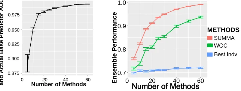
out of 30 base classifiers thirty times and calculated the mean and standard error of the mean AUC associated with the WOC ensemble. Figure 1b shows that the SUMMA en-semble increases in performance more readily as classifiers are added in the enen-semble and saturates at a higher AUC than the WOC ensemble (Figure 1b). Moreover, we see that the SUMMA performance saturates at n= 15 classifiers suggesting that we can achieve a performance close to that of the full ensemble with only 15 classifiers (or 50% of all the base classifiers). We leave the investigation of finding an optimal number of classifiers for the ensemble construction for future research.
0.875 0.900 0.925 0.950 0.975 0 60
Correlation between Predicted and Actual Base Predictor A
UC
Number of Methods20 40
(a) Correlation between the SUMMA inferred AUC of the base classifiers and their actual AUC, as a function of the number of base classifiers
0.7 0.8 0.9 1.0
0 20 40 60
Ensemble Performance
METHODS SUMMA
Number of Methods
WOC Best Indv
(b) AUC of the SUMMA ensemble as a func-tion of the number of base classifiers
In the second part of the analysis, we empirically tested the dependence of SUMMA on varying number of classifiers, samples, and class prevalence. In each case we change only one of the simulation parameter from their default values of, M = 30 base classifiers,
N = 1000 samples, and the prevalence of class 1, ρ = 1/2. The error bars in the figures represents the standard error of the mean for 30 repeated experiments.
First, we tested the influence of the number of classifiers by simulating predictions and applying SUMMA to ensembles composed of M = {5,6,7, . . . ,60} base classifiers. This experiment is different from the analysis of Fig 1.b, because here we run SUMMA using
M = {5,6,7, . . . ,60} (Fig. 2a) base classifiers as opposed to using the same covariance
matrix of all 30 base classifiers as done in the experiments leading to Fig 1.b. In other words, the inference of weights is done for each set ofM classifiers as opposed to the earlier analysis. Intuitively, inferring ∆ for larger covariance matrices should become more accurate because the number of equations grows faster,M(M−1)/2, than the number of parameters ∆i,M. Indeed, this intuition is confirmed in Figure 2. We see that the correlation between the predicted versus actual AUC of base classifiers inferred by SUMMA forM = 5 is≈0.87, and increases readily to ≈0.97 for M ≥15. We then tested how the number of classifiers affected the performance of the corresponding SUMMA ensemble. In Figure 2b we find that the SUMMA ensemble outperforms the WOC and best individual performing classifier in the ensemble. Moreover, as the number of classifiers increases, SUMMA’s performance increases towards the perfect AU C = 1 even if the best individual classifier AUC never exceeds 0.75.
Next, we tested how the number of samples affect the performance of SUMMA. From the law of large numbers, one would expect that the performance of SUMMA would improve with the number of samples. This is simply because the error in estimating the covariance matrix elements decreases with N which in turn results in a more reliably estimate of the AUCs of base classifiers. Indeed, in Figure 3a we see that the correlation between the SUMMA inferred AUC and the actual AUC of base classifiers monotonically increases from ≈0.57 to ≈1 when increasing N from 30 to 4000 samples. Furthermore, the AUC of the SUMMA ensemble is also increasing with the number of samples mainly due to the fact that we can estimate the performance of base classifiers more reliably with increasing sample size (Figure 3a). Note that the WOC performance is not much affected by the sample size. When we have a very small number of samples (N <= 50) the uncertainty in the estimated performances of base classifiers is large enough to negatively influence the SUMMA ensemble performance as shown in Figure 3b. In such cases the WOC ensemble can be preferred to SUMMA. However, when (N > 50) the SUMMA ensemble performs significantly better than the WOC ensemble.
0.4 0.6 0.8 1.0
0 1000 3000 4000
Number of Samples
Correlation between
Predicted
and Actual Base Predictor A
UC
2000
(a) Correlation between the SUMMA in-ferred AUC of the base classifiers and their actual AUC, as a function of the number of samples
0.7 0.8 0.9
0 1000 3000 4000
Number of Samples
Ensemble Performance
METHODS
SUMMA WOC Best Indv
2000
(b) AUC of the SUMMA ensemble as a function of the number of samples
Figure 3: The dependence of the SUMMA results with the number of samples for M = 30 base classifiers and positive class prevalence ρ= 0.5.
0.90 0.95
Correlation between Predicted and Actual Base Predictor AUC Prevalence of Positive Class 1.00
1.00 0.75 0.50 0.25 0.80
(a) Correlation between the SUMMA in-ferred AUC of the base classifiers and their actual AUC, as a function of the preva-lence of the positive class
0.70 0.75 0.80 0.85 0.90 0.95
0.25 0.50 0.75
Prevalence of Positive Class
Ensemble Performance
METHODS
SUMMA
1.00
WOC Best Indv
(b) AUC of the SUMMA ensemble as a function of the prevalence of the positive class
Figure 4: The dependence of the SUMMA results with the prevalence of the positive class
ρ forM = 30 base classifiers and N = 1000 samples
7.2. Inference of genes targeted by a transcriptional regulator: The BCL6 DREAM Challange
find-ing efficient solutions to challengfind-ing real life problems. The diversity of machine learnfind-ing strategies applied by challenge participants in these competitions results in a large number of independent predictions for the same test set which can be aggregated into an ensemble prediction with methods such as SUMMA. In this section we will use one such competition, the DREAM BCL6 challenge (Stolovitzky et al., 2009) to test the performance of SUMMA. DREAM Challenges lend themselves for this task because after the finalization of the com-petitions, DREAM organizers share the gold standard labels associated with the test set as well as the collection of participants’ algorithms and predictions. This allowed us to objectively evaluate the performance of SUMMA in a problem of biological interest.
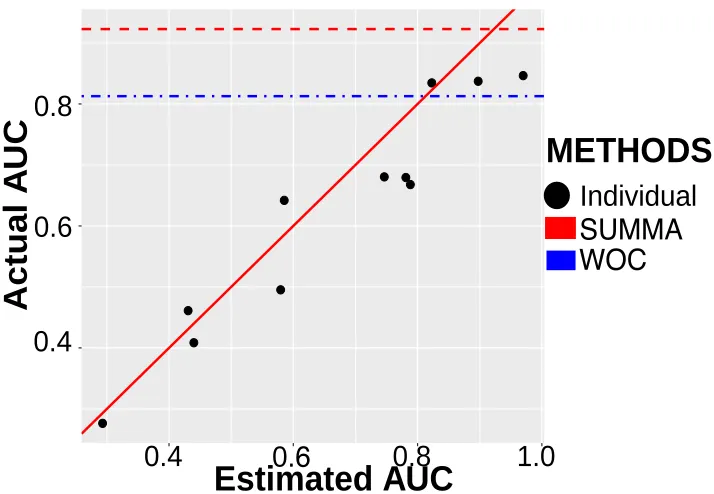
In the BCL6 challenge, participants were asked to infer whether the activity of a given gene is regulated, or in biological jargon: is targeted, by the transcription factor BCL6. The participants were provided an unlabeled feature matrix consisting of micro array mea-surements, with each element representing the relative abundance of RNA transcripts cor-responding to a specific gene and given a specific perturbation. Additionally, they were allowed to incorporate any additional data that could be of use. They were then asked to report the confidence scores, in rank order for 200 genes, indicating whether a gene was a target of BCL6. Hidden from the participants were the experimentally determined class labels for each gene, in which 53 of the 200 (ρ= 0.265) genes were determined to be targets of BCL6. This way of creating gold standard labels is typical in biology and is very expen-sive both in monetary value as well as human resources. Therefore, the BCL6 challenge is a perfect application of SUMMA where there is no labeled data readily available for training. Eleven teams participated and submitted predictions to this challenge. Therefore, the input to SUMMA was a matrix of size 200 genes by 11 methods, the elements of which are confidence scores between 0 and 1. We used the gold standard labels created by the organizers to compare the performance of SUMMA to that of individual methods, as well as to other methods including the Spectral Meta Learner (SML) algorithm (Parisi et al., 2014), the WOC and an unsupervised classifier based on k-means clustering.
We first tested the ability of SUMMA to estimate the AUCs of individual classifiers. As seen in Figure 5, SUMMA could reliably estimate the performance of individual classifiers with a correlation of 0.96 between the inferred and actual AUCs. Figure 5 also shows the AUC of the SUMMA ensemble, obtained by ranking samples according to the SUMMA scorecSU M M A
0.4
0.6
0.8
0.4
0.8
1.0
Estimated AUC
Actual A
UC
METHODS
Individual
0.
6
SUMMA
WOC
Figure 5: Comparison between the SUMMA inferred AUC on the BCL6 data and the actual AUC of the base 11 base classifiers
though confidence values are provided in the interval [0,1], it is likely that their distribu-tion and interpretadistribu-tion is different in each predicdistribu-tion, which may have a negative impact in confidence score aggregation. Our results show that in situations in which we don’t have control on the generation of confidence scores by classifiers or do not have labeled data to re-calibrate outputs of base classifiers, rank transformation allows for a robust way of normalizing confidence scores.
Method Balanced Accuracy
SUMMA 0.82
SML 0.8
Best Individual 0.79 Second Best Individual 0.66
k-means (k=2) 0.52
Table 1: The performance (balance accuracy) of ensemble methods and the two best indi-vidual methods used to solve the BCL6 DREAM Challenge
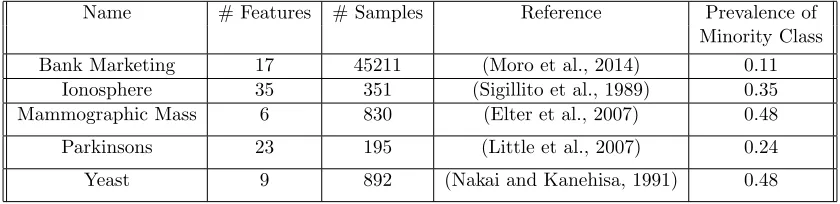
Name # Features # Samples Reference Prevalence of Minority Class Bank Marketing 17 45211 (Moro et al., 2014) 0.11
Ionosphere 35 351 (Sigillito et al., 1989) 0.35 Mammographic Mass 6 830 (Elter et al., 2007) 0.48
Parkinsons 23 195 (Little et al., 2007) 0.24
Yeast 9 892 (Nakai and Kanehisa, 1991) 0.48
Table 2: Summary of Real World Data Sets from UCI Machine Learning Repository
7.3. Applying SUMMA to Real World Data in Diverse Domains
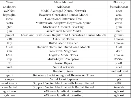
Name Main Method RLibrary
adaboost Adaboost fastAdaboost
avNNet Model Averaged Neural Network nnet
bayesglm Bayesian Generalized Linear Model arm
ctree Conditional Inference Tree party
earth Multivariate Adaptive Regression Spline earth
gbm Stochastic Gradient Boosting gbm
glm Generalized Linear Model stats
glmnet Lasso and Elastic-Net Regularized Generalized Linear Models glmnet
J48 C4.5-like Trees RWeka
Jrip Rule-Based Classifier RWeka
C5.0 Decision Trees and Rule-Based Models C50
knn k-Nearest Neighbors kknn
LMT Logistic Model Trees RWeka
mlp Multi-Layer Perceptron RSNNS
nb Naive Bayes klaR
nnet Neural network nnet
rf Random Forest randomForest
rpart Recursive Partitioning and Regression Trees rpart
simpls Partial Least Squares pls
svmLinear2 Support Vector Machine with Linear Kernel e1071 svmRadial Support Vector Machine with Radial Kernel kernlab
xgbLinear eXtreme Gradient Boosting xgboost
xgbTree eXtreme Gradient Boosting xgboost
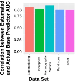
(0.96). This is likely due to the conditional dependence between base classifiers. Table 4 shows the ranking of classifiers including SUMMA ensemble in terms of AUC. We can easily observe that classifiers that perform best in one data set do not necessarily perform well in other data sets. In fact, they can be one of the worst in other data sets. This is most likely due to the distributions of the data being different in different data sets and classifiers with different theoretical backgrounds are more suitable to be applied in one type of data than other. In comparison, SUMMA performs better than the best individual classifier in the Bank Marketing, Parkinsons and Yeast datasets, and second best in the mammographic masses and fifth in ionosphere data sets. Next, for two of the datasets, Bank Marketing and Yeast, we analyzed how the number of integrated classifiers affects the performance of SUMMA prediction by examining randomly sampled combinations of individual classifiers (Figures 7a and b respectively). SUMMA performs better than individual classifiers even when integrating small sets of individual predictions. Performance increases further with the number of integrated classifiers. For instance, for 15 randomly selected individual classifiers, the SUMMA ensemble performs better than the best amongst the 15 classifiers in 98% of the cases in the Bank Marketing data set and it ranks best in 80% of the cases and best or second best in 97% of the cases in the Yeast data set demonstrating the robustness of SUMMA. Table 5 shows the frequency with which SUMMA outperforms the WOC ensemble prediction in the Bank Marketing and Yeast data. For example, for the Bank Marketing data set if we combine random 10 teams, 99% of the times SUMMA performs better than WOC. For the Yeast data, SUMMA gives a better prediction than WOC in about 65% of the times.
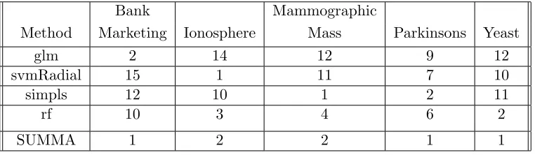
We next compared the classification accuracy of SUMMA to individual classifiers. For that we used the binary label predictions output by caret and computed the balanced accuracy of each individual classifier. Table 4 shows the ranking of classifiers including SUMMA ensemble in terms of their balanced accuracies. Similar to the rank based outputs, SUMMA is better than the best in 3 of the 5 datasets and is the second best in the rest. Moreover, as before classifiers that perform best in one data set do not necessarily perform well in other data sets.
0.00
0.25
0.50
0.75
0.88
Bankmarketing
Ionosphere
Mammographic Masses
Parkinsons
Y
east
Data Set
Correlation between
Estumated
and Actual Base Predictor AUC
Figure 6: Correlation between the actual and estimated AUC of the base classifiers tested on the six UCI datasets considered in this paper.
60 70 80 90
0.00 0.25 0.50 0.75 1.00
Top x % of individual methods
Probability to be in top
x %
# of Methods
5 10 15 20 100
(a) Bank Marketing Data
60 70 80 90
0.00 0.25 0.50 0.75 1.00
Top x % of individual methods
Probability to be in top
x %
100
# of Methods
5 10 15 20
(b) Yeast Data
Figure 7: Robustness of SUMMA with increasing number base classifiers (Y axis represents how often SUMMA is in the topx% of methods)
8. Conclusions
Bank Mammographic
Method Marketing Ionosphere Mass Parkinsons Yeast
Earth 2 22 5 6 6
svmRadial 12 1 18 5 5
gbm 5 7 1 4 4
C5.0 8 8 7 2 21
rf 7 3 6 5 2
SUMMA 1 5 2 1 1
Table 4: Ranking of the different methods in each application domain. Only the classifiers that ranked first in at least one application are listed.
% SUMMA is better than WOC Number Classifiers Bank Marketing Data Yeast Data
5 90 69
10 99 68
15 100 63
20 100 68
Table 5: Percentage of times SUMMA outperforms WOC.
Bank Mammographic
Method Marketing Ionosphere Mass Parkinsons Yeast
glm 2 14 12 9 12
svmRadial 15 1 11 7 10
simpls 12 10 1 2 11
rf 10 3 4 6 2
SUMMA 1 2 2 1 1
Table 6: Ranking of Methods using classification performance (Balanced Accuracy) in each application domain. Only the classifiers that ranked first in at least one application are listed.
class labels most likely associated with each sample, as well as a new integrated ranking for the samples from which we can compute the ensemble AUC.
We evaluated the performance of SUMMA on synthetic data, on the predictions submit-ted to a crowd-sourced competition (the BCL6 DREAM Challenge), and on multiple pre-dictions to classification problems arising in real life contexts. The application of SUMMA in different settings shows that SUMMA can reliably estimate the AUCs of base classifiers in idealized problems where the assumption of conditional independence holds, as well as in real life applications where the assumption of conditional independence is likely violated. SUMMA performed better than the best base classifiers in the synthetic data as well as the BCL6 DREAM Challenge. In a third application, we used five datasets available from UCI machine learning repository which we split into a training set to train base classifiers and a test set to run ensemble methods including SUMMA. Our results show that SUMMA performs better than the best performer in three of the five datasets and among the top performers in the other cases.
In this paper we have introduced SUMMA for a binary classification problem. SUMMA can be extended to multi-class classification problems as follows. Assume that each classifier in an ensemble provides a score (such as confidence level or the distance to a surface) associated to the assignment of each sample to each of k > 2 classes. For each class iwe run SUMMA as a binary classification problem, with classibeing the positive class and all the otherk−1 classes constituting the negative class. In this way, for each classiand each sample j we have a SUMMA score Sij. A multi-class classification extension of SUMMA would consist of assigning sample j the class i that makes Sij maximum. This approach requires that the classifiers assign class scores independently given the positive and negative class in each of thek binary problems.
SUMMA could be extended to cases where the conditional independence assumption between the classifiers does not hold and there is some structured correlation in the pre-dictions. An example could be a block structure where a group of classifiers are correlated with each other but uncorrelated with predictors in other groups. A first step in that di-rection would be developing a method to identify the block structure and then average the predictions in each block before running SUMMA.
Another extension of our work would be to develop a modified version of SUMMA for the so-called rank-aggregation problem which is a very active area of research (Bhowmik and Ghosh, 2017). In the rank-aggregation problem, there is an unknown but true ordering of samples and each method is trying to predict this unknown ordering. The performance of a method is measured using various quantities such asKendall-taudistance (Klementiev et al., 2008). In fact, one of the well established baseline methods used is Borda-counting which is strongly connected to the SUMMA score as we showed in the manuscript (Bhowmik and Ghosh, 2017). The first step towards this direction is determining the right performance metric to be used and setting up the right assumptions under which it can be estimated.
References
Javed A Aslam and Mark Montague. Models for metasearch. In Proceedings of the ACM SIGIR Conference, 2001.
Akshay Balsubramani and Yoav Freund. Scalable semi-supervised aggregation of classifiers. In Advances in Neural Information Processing Systems, 2015.
Rina Foygel Barber and Wooseok Ha. Gradient descent with non-convex constraints: local concavity determines convergence. Information and Inference, 7(4):755–806, 2018.
Antonio Bella, C`esar Ferri, Jos´e Hern´andez-Orallo, and Mar´ıa Jos´e Ram´ırez-Quintana. On the effect of calibration in classifier combination. Applied Intelligence, 38(4):566–585, 2013.
Avradeep Bhowmik and Joydeep Ghosh. Letor methods for unsupervised rank aggregation. In Proceedings of the International Conference on World Wide Web, 2017.
Leo Breiman. Bagging predictors. Machine Learning, 24(2):123–140, 1996.
Jian-Feng Cai, Emmanuel J Cand`es, and Zuowei Shen. A singular value thresholding algo-rithm for matrix completion. SIAM Journal on Optimization, 20(4):1956–1982, 2010.
Emmanuel J Cand`es and Benjamin Recht. Exact matrix completion via convex optimiza-tion. Foundations of Computational Mathematics, 9(6):717, 2009.
Emmanuel J Cand`es and Terence Tao. The power of convex relaxation: Near-optimal matrix completion. IEEE Transactions on Information Theory, 56(5):2053–2080, 2010.
Rich Caruana, Alexandru Niculescu-Mizil, Geoff Crew, and Alex Ksikes. Ensemble selection from libraries of models. In Proceedings of the International Conference on Machine learning, 2004.
Fran¸cois Chollet. Xception: Deep learning with depthwise separable convolutions. In Pro-ceedings of the IEEE Conference on Computer Vision and Pattern Recognition, pages 1251–1258, 2017.
Corinna Cortes and Vladimir Vapnik. Support-vector networks. Machine Learning, 20(3): 273–297, 1995.
Alexander Philip Dawid and Allan M Skene. Maximum likelihood estimation of observer error-rates using the em algorithm. Journal of the Royal Statistical Society: Series C, 28 (1):20–28, 1979.
Arthur P Dempster, Nan M Laird, and Donald B Rubin. Maximum likelihood from incom-plete data via the em algorithm. Journal of the Royal Statistical Society: Series B, 39 (1):1–22, 1977.
Thomas G Dietterich. Ensemble learning. The Handbook of Brain Theory and Neural Networks, 2:110–125, 2002.
Carl Eckart and Gale Young. The approximation of one matrix by another of lower rank.
M Elter, R Schulz-Wendtland, and T Wittenberg. The prediction of breast cancer biopsy outcomes using two cad approaches that both emphasize an intelligible decision process.
Medical Physics, 34(11):4164–4172, 2007.
Peter Emerson. The original borda count and partial voting. Social Choice and Welfare, 40(2):353–358, 2013.
Yoav Freund and Robert E Schapire. A decision-theoretic generalization of on-line learning and an application to boosting.Journal of Computer and System Sciences, 55(1):119–139, 1997.
Wei Gao, Rong Jin, Shenghuo Zhu, and Zhi-Hua Zhou. One-pass auc optimization. In
International Conference on Machine Learning, 2013.
Mike Gashler, Christophe Giraud-Carrier, and Tony Martinez. Decision tree ensemble: Small heterogeneous is better than large homogeneous. In Proceedings of International Conference on Machine Learning and Applications, 2008.
Frank E Harrell. Ordinal logistic regression. InRegression Modeling Strategies, pages 331– 343. Springer, 2001.
Ariel Jaffe, Boaz Nadler, and Yuval Kluger. Estimating the accuracies of multiple classifiers without labeled data. In Artificial Intelligence and Statistics, 2015.
Prateek Jain and Sewoong Oh. Learning mixtures of discrete product distributions using spectral decompositions. In Conference on Learning Theory, 2014.
Prateek Jain, Raghu Meka, and Inderjit S Dhillon. Guaranteed rank minimization via singular value projection. In Advances in Neural Information Processing Systems, pages 937–945, 2010.
Edwin T Jaynes. Information theory and statistical mechanics. Physical Review, 106(4): 620, 1957.
Azam Karami, Mehran Yazdi, and Gr´egoire Mercier. Compression of hyperspectral images using discerete wavelet transform and tucker decomposition. IEEE Journal of Selected Topics in Applied Earth Observations and Remote Sensing, 5(2):444–450, 2012.
Alexandre Klementiev, Dan Roth, and Kevin Small. Unsupervised rank aggregation with distance-based models. InProceedings of the International Conference on Machine Learn-ing, 2008.
Tamara G Kolda and Brett W Bader. Tensor decompositions and applications. SIAM Review, 51(3):455–500, 2009.
Max Kuhn et al. Building predictive models in r using the caret package. Journal of Statistical Software, 28(5):1–26, 2008a.
Max Kuhn et al. Caret package. Journal of Statistical Software, 28(5):1–26, 2008b.
Max A Little, Patrick E McSharry, Stephen J Roberts, Declan AE Costello, and Irene M Moroz. Exploiting nonlinear recurrence and fractal scaling properties for voice disorder detection. BioMedical Engineering Online, 6(1):23, 2007.
Tie-Yan Liu, Hang Li, and Yu-Ting Liu. Supervised rank aggregation based on rankings, 2010. US Patent 7,840,522.
Daniel Marbach, James C Costello, Robert K¨uffner, Nicole M Vega, Robert J Prill, Diogo M Camacho, Kyle R Allison, Andrej Aderhold, Richard Bonneau, Yukun Chen, et al. Wis-dom of crowds for robust gene network inference. Nature methods, 9(8):796, 2012.
Caren Marzban. The roc curve and the area under it as performance measures. Weather and Forecasting, 19(6):1106–1114, 2004.
S´ergio Moro, Paulo Cortez, and Paulo Rita. A data-driven approach to predict the success of bank telemarketing. Decision Support Systems, 62:22–31, 2014.
Kenta Nakai and Minoru Kanehisa. Expert system for predicting protein localization sites in gram-negative bacteria. Proteins: Structure, Function, and Bioinformatics, 11(2): 95–110, 1991.
Alexandru Niculescu-Mizil, Claudia Perlich, Grzegorz Swirszcz, Vikas Sindhwani, Yan Liu, Prem Melville, Dong Wang, Jing Xiao, Jianying Hu, Moninder Singh, et al. Winning the kdd cup orange challenge with ensemble selection. In Proceedings of the International Conference on KDD-Cup, 2009.
Shmuel Nitzan and Jacob Paroush. Optimal decision rules in uncertain dichotomous choice situations. International Economic Review, pages 289–297, 1982.
Shmuel Nitzan and Ariel Rubinstein. A further characterization of borda ranking method.
Public Choice, 36(1):153–158, 1981.
T Maruthi Padmaja, Narendra Dhulipalla, Raju S Bapi, and P Radha Krishna. Unbalanced data classification using extreme outlier elimination and sampling techniques for fraud detection. In Proceedings of the International Conference on Advanced Computing and Communications, 2007.
Fabio Parisi, Francesco Strino, Boaz Nadler, and Yuval Kluger. Ranking and combining multiple predictors without labeled data. Proceedings of the National Academy of Sci-ences, 111(4):1253–1258, 2014.
Robert J Prill, Daniel Marbach, Julio Saez-Rodriguez, Peter K Sorger, Leonidas G Alex-opoulos, Xiaowei Xue, Neil D Clarke, Gregoire Altan-Bonnet, and Gustavo Stolovitzky. Towards a rigorous assessment of systems biology models: The dream3 challenges. PloS One, 5(2):e9202, 2010.
Robert E Schapire. The strength of weak learnability. Machine Learning, 5(2):197–227, 1990.
Amartya Sen. Social choice theory. Handbook of Mathematical Economics, 3:1073–1181, 1986.
Vincent G Sigillito, Simon P Wing, Larrie V Hutton, and Kile B Baker. Classification of radar returns from the ionosphere using neural networks. Johns Hopkins APL Technical Digest, 10(3):262–266, 1989.
Rion Snow, Brendan O’Connor, Daniel Jurafsky, and Andrew Y Ng. Cheap and fast—but is it good?: evaluating non-expert annotations for natural language tasks. InProceedings of the conference on empirical methods in natural language processing, pages 254–263. Association for Computational Linguistics, 2008.
Gustavo Stolovitzky, Robert J Prill, and Andrea Califano. Lessons from the dream2 chal-lenges: a community effort to assess biological network inference. Annals of the New York Academy of Sciences, 1158(1):159–195, 2009.
Karthik Subbian and Prem Melville. Supervised rank aggregation for predicting influencers in twitter. In Proceedings of the International Conference on Privacy, Security, Risk and Trust, 2011.
Liang Sun, Tomonori Honda, Vesselin Diev, Gregory Gancarz, Jeong-Yoon Lee, Ying Liu, Mona Mahmoudi, Raghav Mathur, Shahinur Rahman, Steve Wickert, et al. Maximize auc in default prediction: Modeling and blending.
James Surowiecki. The wisdom of crowds. Anchor, 2005.
Chih-Fong Tsai and Yu-Chieh Hsiao. Combining multiple feature selection methods for stock prediction: Union, intersection, and multi-intersection approaches. Decision Sup-port Systems, 50(1):258–269, 2010.
Lieven Vandenberghe and Stephen Boyd. Applications of semidefinite programming.Applied Numerical Mathematics, 29(3):283–299, 1999.
Sean Whalen and Gaurav Pandey. A comparative analysis of ensemble classifiers: case studies in genomics. In Proceedings of the International Conference on Data Mining, 2013.
David H Wolpert. Stacked generalization. Neural Networks, 5(2):241–259, 1992.
Appendix A. Details of SDP Approach
A.1. Semi-Definite Programming
We start this section by the following definition.
Definition 9 We say that a matrix Q is off-diagonal rank-one if there exists a vector q
and a diagonal matrix D s.t.
Q=qqT +D. (28)
In order to show that R is the unique solution to the problem (11), we prove a lemma stating that a unique solution of the problem (11) exists for an arbitrary matrix Q whose off-diagonal elements coincide with a rank one matrix. The application of this lemma with
Q= Σ2 will then allow us to show the desired result.
Lemma 10 Let Q be an off-diagonal rank-one square matrix of size M such that
Q=qqT +D0, (29)
for someq ∈RM withM ≥3, and diagonal matrixD
0 and assume thatq1, q2, q36= 0. Then
the optimization problem
min
D rank(Q−D) s.t. D(i, j) = 0 for i6=j, and Q−D0, (30)
has the unique solution D0, with Q−D0 =qqT = (−q)(−q)T so that we can recover q up
to its sign.
Proof Let Q be defined as in Equation (29) with q1, q2, q3 6= 0 andD0. Since Q(i, j) =
qiqj 6= 0, it is obvious that for any diagonal matrixD,Q−D6= 0. Hence,rank(Q−D)>0 for any diagonal matrix D. Moreover, sinceQ−D0=qqT one solution of the optimization problem in Equation (11) isD0. Next, we show that D0 is the only diagonal matrix that is a feasible point of the optimization problem.
Suppose there exists a diagonal matrix Ds such that Ds 6=D0 and rank(Q−Ds) = 1. Then sinceQ−Ds is symmetric, there exists s∈RM such that Q−Ds =ssT and q 6=s. Since bothD0 and Ds are diagonal andDs+ssT =Q=D0+qqT, then the equality
qiqj =sisj. (31)
must be true for alli6=j wherei, j∈ {1,2, . . . , M}.
Without loss of generality lets assume that q1 6= 0> s1 6= 0. Equation (31) for (i, j) = (1,2) implies that s2 > q2, and for (i, j) = (1,3) implies that s3 > q3. Under these inequalities, when (i, j) = (2,3) we see that s2s3 > q2q3, which contradicts equation (31). Therefore, q1 = s1 which from Equation (31) implies that for all i, qi = si. Therefore,
D0=Ds and consequentlyD0 is the unique solution to the optimization problem given in equation (11).
As we discussed in the main text the optimization problem in (30) can be relaxed to the following SDP:
min
Theorem 11 Suppose thatQ is an M×M matrix of the form given in Equation (29) for some q and diagonal matrix D0, then the optimization problem in Equation (32) has the
unique solution D0, provided that
q2i <X
j6=i
q2j, ∀i∈ {1,2, . . . , M}. (33)
Moreover, Q−D0 =qqT so that we can recover q up to its sign.
Proof LetDbe an arbitrary diagonal matrix such thatQ−Dis a PSD (Positive Semidef-inite) matrix. Then the eigenvalues of Q−D are non-negative and equal to the singular values ofQ−D. Combined with the fact that the trace of a matrix is equal to the sum of its eigenvalues, we know the following:
kQ−Dk∗ =T r(Q−D).
Without loss of generality lets assume that the diagonal entries of Q are equal to 0, that is Q=qqT −diag(qqT). In this case, note that D0 =−diag(qqT) is a feasible solution for the optimization problem in Equation (13). Next let D be an arbitrary solution and since
Q−Dis PSD,Dii≤0 for alli. Suppose for someiwe haveDii>−q2i and for allj6=iwe have Djj ≥ −q2j. Forj 6=i, consider the following sub-matrix ofQ−D,
(Q−D)ij =
−Dii qiqj
qiqj −Djj
.
Since det((Q−D)ij) =DiiDjj −qi2q2j <0, the submatrix (Q−D)ij of Q−D is negative definite which contradicts the fact that Q−D is PSD. Therefore, combined with the fact that Dii ≤0 for eachi, this implies that in order for a diagonal matrixD to be a feasible point for the optimization problem (13)
1. Either for all i, we haveDii≤ −qi2
2. Or there existisuch that Dii>−qi2, and ∀j6=i Djj ≤ −qj2.
SupposeDis a feasible point that satisfies condition 1, thenT r(Q−D)≥T r(Q+diag(qqt)) for every feasible D. Hence, D0 = −diag(qqt) remains to be the unique solution of the optimization problem. Now suppose there exists a feasible point D such that condition 2 of above is satisfied. Then WLO assume that D11>−q12 and Djj ≤ −qi2 forj ≥2. Next, for each j≥2 consider the following submatrix:
(Q−D)1j =
−D11 q1qj
q1qj −Djj
.
In order for Q−Dto be PSD, we should havedet((Q−D)1j) =D11Djj−q12qj2>0, which in turn implies that
Djj <
q12qj2 D11