www.geosci-model-dev.net/5/433/2012/ doi:10.5194/gmd-5-433-2012
© Author(s) 2012. CC Attribution 3.0 License.
Geoscientific
Model Development
Development and evaluation of a building energy model integrated
in the TEB scheme
B. Bueno1,2, G. Pigeon1, L. K. Norford2, K. Zibouche3, and C. Marchadier1
1CNRM-GAME, URA1357, CNRS – M´et´eo France, Toulouse, France 2Massachusetts Institute of Technology, Cambridge, USA
3Universit´e Paris-Est, Centre Scientifique et Technique du Bˆatiment (CSTB), France Correspondence to: B. Bueno ([email protected])
Received: 13 September 2011 – Published in Geosci. Model Dev. Discuss.: 15 November 2011 Revised: 5 March 2012 – Accepted: 19 March 2012 – Published: 29 March 2012
Abstract. The use of air-conditioning systems is expected to increase as a consequence of global-scale and urban-scale climate warming. In order to represent future scenarios of ur-ban climate and building energy consumption, the Town En-ergy Balance (TEB) scheme must be improved. This paper presents a new building energy model (BEM) that has been integrated in the TEB scheme. BEM-TEB makes it possi-ble to represent the energy effects of buildings and building systems on the urban climate and to estimate the building en-ergy consumption at city scale (∼10 km) with a resolution of a neighbourhood (∼100 m). The physical and geometric definition of buildings in BEM has been intentionally kept as simple as possible, while maintaining the required fea-tures of a comprehensive building energy model. The model considers a single thermal zone, where the thermal inertia of building materials associated with multiple levels is repre-sented by a generic thermal mass. The model accounts for heat gains due to transmitted solar radiation, heat conduc-tion through the enclosure, infiltraconduc-tion, ventilaconduc-tion, and inter-nal heat gains. BEM allows for previously unavailable so-phistication in the modelling of air-conditioning systems. It accounts for the dependence of the system capacity and ef-ficiency on indoor and outdoor air temperatures and solves the dehumidification of the air passing through the system. Furthermore, BEM includes specific models for passive sys-tems, such as window shadowing devices and natural ven-tilation. BEM has satisfactorily passed different evaluation processes, including testing its modelling assumptions, veri-fying that the chosen equations are solved correctly, and val-idating the model with field data.
1 Introduction
The energy consumption of heating, ventilation and air-conditioning (HVAC) systems in buildings has become an important factor in the design and analysis of urban areas. HVAC systems are responsible for waste heat emissions that can contribute (among other causes) to the increase in air temperature observed in urban areas with respect to their un-developed rural surroundings (Bueno et al., 2012; de Munck et al., 2012). This increase in air temperature in cities, a phe-nomenon known as the urban heat island (UHI) effect, can af-fect the energy consumption of HVAC systems and the waste heat emissions associated with them. The use of HVAC sys-tems is expected to increase in the following years as a con-sequence of global-scale and urban-scale climate warming (Adnot, 2003); therefore, urban climate models, such as the Town Energy Balance (TEB) scheme (Masson, 2000), must be improved in order to represent future scenarios of climate conditions and energy consumption in urban areas.
minimum indoor air temperature threshold is used to calcu-late the heating loads of the building associated with trans-mission through building surfaces (Pigeon et al., 2008).
In order to improve the representation of buildings in TEB, we have considered two different approaches. The first ap-proach is to couple a well-known building energy model, such as EnergyPlus (Crawley et al., 2001), with TEB. This is the strategy adopted in Bueno et al. (2011). However, the coupled scheme (CS) developed in this study requires a num-ber of iterations between the two models, which makes it un-suitable for coupling with atmospheric models.
The second approach is to develop a new building energy model (BEM) integrated in the urban canopy model. This is the method used by Kikegawa et al. (2003) and Salamanca et al. (2010). They developed simplified building energy models that are able to capture the main heat transfer pro-cesses that occur inside buildings and to calculate building energy demand, HVAC energy consumption and waste heat emissions (Kondo and Kikegawa, 2003; Salamanca and Mar-tilli, 2010; Kikegawa et al., 2006; Ihara et al., 2008). How-ever, they consider idealized HVAC systems and do not take into account passive building systems. Following the same method, this paper presents a BEM integrated in the TEB model that overcomes the limitations of the previous models. In this study, BEM-TEB is evaluated at three levels: mod-elling assumptions; model verification, based on a son with the CS; and model validation, based on a compari-son with field data from two experiments, Toulouse (Mascompari-son et al., 2008) and Athens (Synnefa et al., 2010).
2 Model description
2.1 Objective and main features
BEM-TEM constitutes a new version of the urban canopy model TEB, in which the energy effects of buildings in the urban climate are better represented. The new version of the model makes it possible to calculate building energy consumption at city or neighbourhood scale. Previous ver-sions of TEB could not calculate cooling energy consump-tion of buildings and the waste heat emissions associated with HVAC systems.
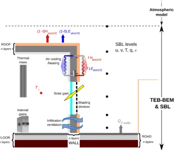
BEM calculates the energy demand of a building by apply-ing a heat balance method. It considers a sapply-ingle thermal zone and represents the thermal inertia of various building levels by a generic thermal mass. The model accounts for solar ra-diation through windows, heat conduction through the enclo-sure, internal heat gains, infiltration and ventilation (Fig. 1).
BEM includes specific models for active and passive building systems. It considers the dependence of the cool-ing system efficiency on indoor and outdoor temperatures and solves the dehumidification of the air passing through the system. Passive building systems such as window shadowing devices and natural ventilation are represented in BEM.
The model has been kept as simple as possible, while maintaining the required features of a comprehensive build-ing energy model. We have intentionally avoided detailed building calculations that would have affected the computa-tional efficiency of the TEB model without providing a sig-nificant gain in accuracy.
2.2 Geometry and building definition
BEM uses the same geometric principles as the TEB model, which can be summarized as:
– Homogenous urban morphology. Building enclosure is defined by an average-oriented fac¸ade and a flat roof. – Uniform glazing ratio. BEM assumes that all building
fac¸ades have the same fraction of glazed surface with respect to their total surface.
In addition, the following is assumed to define buildings in BEM:
– Single thermal zone. BEM assumes that all buildings in a particular urban area have the same indoor air tem-perature and humidity. This approach is justified if the objective is to calculate the overall energy consumption of a building (or neighbourhood), rather than the energy performance of a specific building zone.
– Internal thermal mass. In the single-zone approach, an internal thermal mass represents the thermal inertia of the construction materials inside a building (e.g. sepa-ration between building levels). The transmitted solar radiation and the radiant fraction of internal heat gains are perfectly absorbed by the internal thermal mass and then released into the indoor environment.
– Adiabatic ground floor. The current version of BEM assumes that the surface of the building in contact with the ground is well-insulated.
2.3 Heat balance method
BEM uses a heat balance method to calculate indoor thermal conditions and building energy demand. An energy balance is applied to each indoor surface (si: wall, window, floor, roof, and internal mass), accounting for conduction, convec-tion, and radiation heat components, viz.
Qcd+Qcv+ X
si
Qrd=0. (1)
Fig. 1. Diagram of a building and an urban canyon. The main physical processes included in BEM-TEB are represented: heat storage in
building and urban construction materials, internal heat gains, solar heat fluxes, waste heat from HVAC systems, etc. The diagram also represents the multi-layer version of the TEB scheme (Hamdi and Masson, 2008) and the possibility of coupling it with an atmospheric mesoscale model.
one bounce of radiative heat fluxes between surfaces. The transient heat conduction through massive building elements (walls, floor, roof, and internal mass) is calculated using TEB routines, which are based on the finite difference method.
To calculate the dynamic evolution of indoor air tempera-ture between a cooling and a heating thermal set point, BEM solves a sensible heat balance at the indoor air. The sensi-ble heat balance is composed of the convective heat fluxes from indoor surfaces, the convective fraction of internal heat gains, the infiltration sensible heat flux, and the sensible heat flux supplied by the HVAC system.
VbldρcpdTdtin=P si
Asihcv,si(Tsi−Tin)
+Qig(1−frd)(1−flat) + ˙Vinfρcp(Turb−Tin) + ˙msyscp Tsys−Tin,
(2)
whereTinis the indoor air temperature;Vbld,ρ, andcpare the
volume, density and specific heat of the indoor air, respec-tively;Asiis the area of the indoor surface; Qig represents
the internal heat gains;flat is the latent fraction of internal
heat gains;frdis the radiant fraction of sensible internal heat
gains;V˙
infis the infiltration air flowrate;Turb is the outdoor
air temperature; andm˙sysandTsysare the mass flowrate and
temperature of the air supplied by the HVAC system. A latent heat balance is also solved to calculate the dy-namic evolution of indoor air humidity. The latent heat bal-ance is composed of the latent fraction of internal heat gains, the infiltration latent heat flux, and the latent heat flux sup-plied by the HVAC system.
Vbldρlv dqin
dt =Qigflat+ ˙Vinfρlv(qurb−qin)+ ˙msyslv qsys−qin
, (3) wherelvis the water condensation heat, andqin,qurbandqsys
are the specific humidity of the indoor air, of the outdoor air, and of the air supplied by the HVAC system, respectively.
The building energy demand is calculated by applying the same sensible and latent heat balances at the indoor air, but assuming that this is at set point conditions. The specific hu-midity set point used for latent energy demand calculations is obtained from the relative humidity set point and the cooling or the heating temperature set point, which are provided by the user.
Qdem,sens= X
si
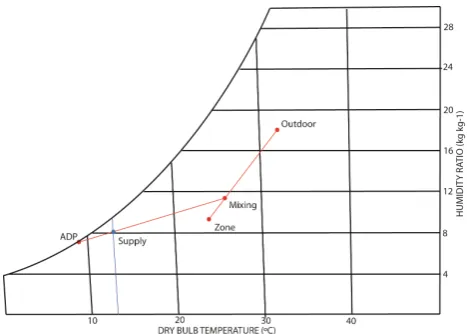
Fig. 2. Psychrometric chart of humid air. The significant points of the HVAC system model for a cooling situation are represented. Zone conditions refer to the temperature and humidity of the indoor air. Recirculated air from the zone is mixed with outdoor air before entering the cooling coil (mixing conditions). The air leaves the cooling coil at supply conditions. The apparatus dewpoint (ADP) is an input of the model and represents the temperature of the air leaving the cooling coil if this would be saturated.
32
Fig. 2. Psychrometric chart of humid air. The significant points
of the HVAC system model for a cooling situation are represented. Zone conditions refer to the temperature and humidity of the indoor air. Recirculated air from the zone is mixed with outdoor air before entering the cooling coil (mixing conditions). The air leaves the cooling coil at supply conditions. The apparatus dewpoint (ADP) is an input of the model and represents the temperature of the air leaving the cooling coil if this would be saturated.
Qdem,lat=Qig,lat+Qinf/vent,lat. (5)
2.4 Windows and solar heat transmission
Window effects have been introduced in the outdoor energy balance of the TEB model. The external surfaces of windows participate in the outdoor energy balance in the same manner as other urban surfaces (walls, road, garden, etc.). Window surfaces are semi-transparent and therefore have three opti-cal properties (albedo, absorptivity, and transmittance). Two coupled surface energy balances are solved to calculate the internal and external surface temperatures of windows. Each surface energy balance accounts for the convective and radia-tive heat fluxes reaching the surface and the steady-state heat conduction through the window.
Building energy models usually consider the dependence of the solar heat transmitted through windows on the angle of incidence of the sun. However, simulations with EnergyPlus for different window orientations show that for an average-oriented canyon, the solar transmittance of windows(τwin)
can be approximated by a uniform value of 0.75 times the solar heat gain coefficient (SHGC) (see Appendix A). The SHGC can be found in window catalogues and represents the fraction of incoming solar radiation that participates in the indoor energy balance. The solar heat transmitted through windows Qsol,win
is then calculated as:
Qsol,win=Qsol,wτwinGR, (6)
where Qsol,w is the solar radiation reaching the building
fac¸ade and GR is the glazing ratio.
The solar absorptivity of windows is calculated as a func-tion of the U-factor and the SHGC, by using the equafunc-tions proposed in EnergyPlus documentation (DOE, 2010). The U-factor can also be found in window catalogues and mea-sures the window conductance, including the convective and longwave heat transfer coefficients at both sides of the win-dow.
The window albedo is calculated so that the three optical properties (albedo, absorptivity, and transmittance) sum to unity. Then, the model uses an area-averaged fac¸ade albedo to calculate solar reflections by weighting the albedo of walls and windows with the glazing ratio of buildings.
2.5 Passive building systems
Passive building systems take advantage of the sun, the wind and environmental conditions to reduce or eliminate the need for HVAC systems. Accurate simulation of their effect is sometimes crucial in predicting the overall energy perfor-mance of buildings (e.g. Bueno et al., 2011). Moreover, they are among the strategies promoted by governments through-out the world to reduce the energy consumption and green-house gas emissions of buildings.
2.5.1 Natural ventilation
In residential buildings in summer (especially when an active cooling system is not available), occupants usually open their windows to naturally ventilate indoor spaces. To represent this situation, BEM includes a natural ventilation module, which modifies the indoor air energy balance (Eqs. 2 and 3) by including an outdoor air flowrate term, similarly to the infiltration term. If the conditions are favourable for natural ventilation, the HVAC system is assumed to be turned off at least during one hour. The natural ventilation air flowrate is calculated from a correlation that depends on the outdoor air velocity, the indoor and outdoor air temperatures, and the geometry of buildings and windows (see Appendix A). 2.5.2 Window shades
2.6 HVAC system
2.6.1 Ideal and realistic definitions of an HVAC system
BEM includes both an ideal and a realistic definition of an HVAC system. In the ideal definition, the system capacity is infinite, and the system supplies the exact amount of energy required to maintain indoor thermal and humidity set points. On the contrary, the realistic definition considers a finite ca-pacity that can be provided by the user or calculated by the
autosize function (see Sect. 2.6.7).
In the case of a cooling system, the realistic definition also takes into account the dependence of the system capacity and efficiency on outdoor and indoor conditions. Furthermore, the system efficiency is affected by part-load performance, when the system does not work at its nominal capacity. The realistic definition of the cooling system solves for the dehu-midification of the air passing through the cooling coil. In most HVAC system configurations, the indoor air humidity is not controlled in the same way as the air temperature, so the calculation of the air humidity requires a psychrometric model of the air crossing the system. Figure 2 represents a psychrometric chart of humid air and the significant points of the HVAC model for a cooling situation (summer). 2.6.2 Mixing conditions
To calculate the supply air conditions and the energy con-sumption of the HVAC system, the model first calculates the mixing conditions of the air recirculated from the building and the outdoor air required for ventilation. This calcula-tion is the same for both the cooling and the heating sys-tem models. The mixing ratio (Xmix)is calculated asXmix=
˙
Vventρ/m˙sys, wherem˙sysis the supply air mass flowrate and ˙
Vventis the ventilation air volume flowrate, which are given
by the user (or calculated by the autosize function in the case of the air mass flowrate) . Then, the mixing air temperature and humidity are calculated from the building air tempera-ture and the outdoor air temperatempera-ture as follows:
Tmix=XmixTurb+(1−Xmix)Tin, (7)
and
qmix=Xmixqurb+(1−Xmix)qin. (8)
2.6.3 Cooling system
In the ideal cooling system model, the energy consumption is calculated by adding the sensible and the latent energy demand of the building and dividing by the system coeffi-cient of performance (COP), QHVAC,cool=Qdem,cool/COP.
The supply conditions are then calculated to meet the build-ing energy demand:
Tsys=Tmix−Hdem,cool/ m˙syscp, (9)
and
qsys=qmix−LEdem,cool/ m˙syslv
, (10)
whereHdem,cool andLEdem,cool are the sensible and latent
cooling demand of the building.
In the realistic cooling system model, the model solves a pychrometric model based on the apparatus dewpoint (ADP) temperature. The current version of BEM considers a constant-volume direct-expansion cooling system, but other system configurations can be added in future versions of the model. At each time step, the supply air temperature and hu-midity are calculated by satisfying two conditions. First, the supply point in the psychrometric chart (Fig. 2) must be con-tained in the line connecting the mixing point and the ADP point. Second, the supply temperature should meet the sen-sible energy demand of the building (Eq. 9). If the energy demand of the building is greater than the system capacity, the system capacity is used to calculate the supply tempera-ture.
The system capacity Qcap,sysis calculated from the
nom-inal system capacity multiplied by a coefficient that depends on outdoor and indoor conditions (see Appendix A). The electricity consumption of the cooling coil (QHVAC,sys) is
calculated by the following expression:
QHVAC,sys=Qcap,sysPLRfPLR/COP, (11)
where PLR is the part-load ratio, calculated as the fraction between the energy supplied and the system capacity, and fPLRis a coefficient that depends on the PLR and accounts
for the loss of the system efficiency due to part-load perfor-mance. The actual COP of the system is calculated from the nominal COP (provided by the user) multiplied by a coef-ficient that depends on outdoor and indoor conditions (see Appendix A).
2.6.4 Heating system
The current version of BEM considers a fuel-combustion heating system. Other heating systems, such as heat pumps, can be added in future versions of the model. The supply air temperature of the heating system is calculated to meet the sensible heating energy demand of the building (Eq. 12). If the energy demand of the building is greater than the heating system capacity, the system capacity is used to calculate the supply temperature.
Tsys=Tmix+Hdem,heat/ m˙syscp. (12)
The heating system model assumes that the indoor air hu-midity is not controlled and that the supply air huhu-midity is the same as the mixing humidity (Eq. 8). The energy con-sumption of the heating system is calculated from the ther-mal energy exchanged between the heating system and the indoor air (Qexch,heat) divided by a constant efficiency(ηheat),
provided by the user.
2.6.5 Fan electricity consumption
The fan electricity consumption is calculated from the fol-lowing correlation extracted from EnergyPlus documentation (DOE, 2010):
Pfan= ˙msys1Pfanηfan/ρ, (14)
where1Pfan is the fan design pressure increase, predefined
as 600 Pa; andηfan is the fan total efficiency, predefined as
0.7.
2.6.6 Waste heat emissions
The waste heat released into the environment by a cooling system is given by:
Qwaste,cool=Qexch,cool+QHVAC,cool, (15)
whereQexch,coolis the thermal energy exchanged between
the cooling system and the indoor air, andQHVAC,coolis the
energy consumption of the cooling system (e.g. electricity). The user can specify the sensible-latent split of the waste heat produced by the cooling system, depending on whether the system is air-condensed, water-condensed, or both.
For the heating system, the waste heat flux is related to the energy contained in the combustion gases and is given by: Qwaste,heat=QHVAC,heat−Qexch,heat, (16)
whereQHVAC,heatis the energy consumption of the heating
system (e.g. gas).
2.6.7 Autosize function
For the realistic model of an HVAC system, BEM requires information about the size of the system. The parameters that determine the size of a system are the rated cooling ca-pacity and the maximum heating caca-pacity. For a constant-volume cooling system, the model also requires its design mass flowrate. This information can be provided to the model manually, or it can be automatically calculated by the
auto-size function.
The autosize function first calculates the maximum heat-ing capacity by applyheat-ing a sensible heat balance at the indoor air (Eq. 4), assuming steady-state heat conduction through the enclosure. An equivalent outdoor air temperature is cal-culated as the average between the design minimum air tem-perature (provided by the user) and a generic sky tempera-ture (253 K). The required air flowrate is then obtained from Eq. (17), assuming a supply air temperature of 323 K.
˙
msys,rat=
Qheat,max
cp Tsupply−Theat,target
. (17)
To calculate the rated cooling capacity, the model dynam-ically simulates the building during four days, between 12 July and 15 July. The rated cooling capacity corresponds to the maximum cooling energy required to maintain indoor
set point conditions for the last day of simulation. This dynamic simulation uses a predefined diurnal cycle of out-door air temperature and incoming solar radiation (see Ap-pendix A). Incoming solar radiation depends on the specific location of the urban area, using the solar zenith angle calcu-lated by the TEB model. Outdoor air humidity, air velocity, and air pressure are considered constant during this simula-tion.
Once the rated cooling capacity is calculated, the required air flowrate is obtained assuming a supply air temperature of 287 K. The rated air flowrate will be the maximum of those calculated for cooling and for heating conditions.
3 Model evaluation
3.1 Modelling assumptions
A methodology is proposed to evaluate BEM assumptions. Two models of the same building with different levels of de-tail are compared by simulating them with EnergyPlus. The first model, which is referred as the detailed model (DM), includes the exact geometry of the building enclosure, de-fines each building level as a separate thermal zone, and introduces internal heat gains in terms of people, lighting, and equipment. The second model, which is referred as the simplified model (SM), maintains the assumptions of BEM. It considers a square-base building defined as a single ther-mal zone with internal mass. The building height, vertical-to-horizontal building area ratio, roof-vertical-to-horizontal building area ratio, glazing ratio, construction configuration of the en-closure (materials and layers), total internal heat gains, and infiltration air flowrate are the same as the DM (Table 1).
To avoid orientation-specific results, DM is simulated for eight different orientations, every 45◦, and SM is simu-lated for two different orientations, rotated 45◦between each other. This is due to the fact that SM has a square base and its four fac¸ades are the same. Then, the average results from each set of simulations are compared.
Table 1. Simulation parameters used in the comparison between the simplified EnergyPlus model and the detailed EnergyPlus model of a
Haussmannian building. Property values represent a typical residential building.
Property Value Unit
Vertical-to-horizontal building area ratio 3.14
Building height 21.50 m
Length of the side of the square building plan 27.36 m Roof-to-horizontal building area ratio 0.69
Internal heat gains 5.58 W m−2 Radiant fraction of internal heat gains 0.40
Latent fraction of internal heat gains 0.20 Window solar heat gain coefficient (SHGC) 0.60
Window U-factor 4.95 W m−2K−1 Glazing-to-wall ratio 0.2
Floor height 2.90 m
Infiltration 0.11 ACH
Ventilation 0.43 ACH
Internal mass-to-horizontal building area ratio 12.83 Internal thermal mass construction Concrete (100 mm)
Indoor thermal set points 19–24 ◦C
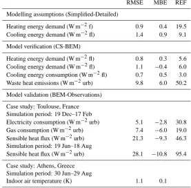
Table 2. Root-mean-square error (RMSE), mean-bias error (MBE), and reference value (REF) of the variables compared in each of the three
evaluation sections. The reference value of energy and heat fluxes is the average of the energy and heat fluxes for the considered time period. The term urb indicates unit of urban area and the term fl indicates unit of used area of the building.
RMSE MBE REF
Modelling assumptions (Simplified-Detailed)
Heating energy demand (W m−2f) 0.9 0.4 19.5 Cooling energy demand (W m−2fl) 1.4 0.9 9.1
Model verification (CS-BEM)
Heating energy demand (W m−2fl) 0.8 0.3 5.6 Cooling energy demand (W m−2fl) 1.1 −0.4 6.0 Cooling energy consumption (W m−2fl) 0.7 0.5 3.0 Waste heat emissions (W m−2urb) 9.8 6.0 50.2
Model validation (BEM-Observations)
Case study: Toulouse, France Simulation period: 19 Dec–17 Feb
Electricity consumption (W m−2urb) 5.1 −2.8 30.8 Gas consumption (W m−2urb) 7.4 −6.0 19.0 Sensible heat flux (W m−2urb) 21.3 −9.3 46.3 Simulation period: 19 Jun–18 Aug
Sensible heat flux (W m−2urb) 28.1 −10.8 95.4 Case study: Athens, Greece
Simulation period: 30 Jun–29 Aug
Fig. 3.
Image of a Haussmannian building in Paris (top). Representation of the detailed model defined
in EnergyPlus (middle). Representation of the simplified model defined in EnergyPlus (bottom).
33
Fig. 3. Image of a Haussmannian building in Paris (top).
Represen-tation of the detailed model defined in EnergyPlus (middle). Repre-sentation of the simplified model defined in EnergyPlus (bottom).
by simulating the upper floor of the building in the SM as a separate thermal zone. This improvement may be considered in future developments of BEM-TEB.
3.2 Model verification
To check that the chosen equations are solved correctly, BEM-TEB is compared to the EnergyPlus-TEB coupled scheme (CS) (Bueno et al., 2011). Table 3 describes the pa-rameters of this case study, which corresponds to the residen-tial urban centre of Toulouse.
Figures 6 and 7 represent the daily average and monthly-averaged diurnal cycles, respectively, of heating energy de-mand in winter and cooling energy dede-mand in summer cal-culated by BEM and the CS. Scores for this comparison are presented in Table 2. The RMSE of heating and cooling energy demand ranges between 0.8 and 1.1 W m−2 of floor area, where the average heating and cooling energy demand calculated by the CS is around 6 W m−2for the same period.
Fig. 4. Daily-average heating (top) and cooling (bottom) energy
de-mand per unit of floor area for winter and summer calculated by the simplified and the detailed EnergyPlus models of a Haussmannian building in Paris.
Fig. 5. Monthly-averaged diurnal cycles of heating energy demand
between 16 January and 15 February (top) and cooling energy de-mand between 1 July and 30 July (bottom) per unit of floor area calculated by the simplified and the detailed EnergyPlus models of a Haussmannian building in Paris.
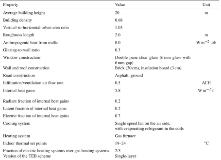
Table 3. Simulation parameters used in the comparison between the coupled scheme and BEM and between BEM and observations. This
configuration represents an urban area composed of residential buildings in the dense urban centre of Toulouse, France.
Property Value Unit
Average building height 20 m
Building density 0.68
Vertical-to-horizontal urban area ratio 1.05
Roughness length 2.0 m
Anthropogenic heat from traffic 8.0 W m−2urb
Glazing-to-wall ratio 0.3
Window construction Double pane clear glass (6 mm glass with 6 mm gap)
Wall and roof construction Brick (30 cm), insulation board (3 cm)
Road construction Asphalt, ground
Infiltration/ventilation air flow rate 0.5 ACH
Internal heat gains 5.8 W m−2fl
Radiant fraction of internal heat gains 0.2
Latent fraction of internal heat gains 0.2
Electric fraction of internal heat gains 0.7
Cooling system Single speed fan on the air side, with evaporating refrigerant in the coils
Heating system Gas furnace
Indoor thermal set points 19–24 ◦C
Fraction of electric heating systems over gas heating systems 2/3 Version of the TEB scheme Single-layer
CS. This can be explained by the fact that the solar radiation model of the TEB scheme tends to overestimate the solar ra-diation reaching building fac¸ades as compared with the CS.
Figure 8 compares the daily average cooling energy con-sumption and waste heat emissions of the HVAC system cal-culated by BEM and the CS. The RMSE of cooling energy consumption is 0.7 W m−2of floor area (Table 2), where the average cooling energy consumption calculated by the CS is 3 W m−2 for the same period. A relative error of 20 % in building energy consumption is acceptable given the state-of-the-art of urban canopy models. Grimmond et al. (2011) show that the surface heat flux error of urban canopy models is usually greater than 20 %. A similar order of magnitude difference is encountered for the waste heat emissions calcu-lated by both models. The RMSE of waste heat emissions is 9.8 W m−2of urban area, where the average waste heat fluxes for the same period is 50.2 W m−2.
3.3 Model validation
Field data from two different experiments are used to eval-uate BEM-TEB. The first one is the CAPITOUL experi-ment, carried out in Toulouse (France) from February 2004 to March 2005 (Masson et al., 2008). Measurements of air tem-perature at street level were carried out simultaneously at 27 locations inside and at the periphery of the city. In this com-parison, the observations from the station located next to the Monoprix building, in the dense urban centre of Toulouse, is used. Forcing information, including sensible heat fluxes, was also measured at the top of the Monoprix building, 47.5 m above the ground. In addition, a city-scale inventory of electricity and natural gas energy consumption of buildings was conducted. Anthropogenic heat fluxes from traffic and building energy uses were obtained from the residual of the surface energy balance (SEB) equation (Oke, 1988). A de-tailed description of the inventory approach and the residual method is presented in Pigeon et al. (2007).
Table 4. Simulation parameters used in the comparison between BEM and observations. This configuration represents an urban area
composed of residential buildings in the Egaleo neighbourhood in Athens, Greece.
Property Value Unit
Average building height 9.5 m
Building density 0.64
Vertical-to-horizontal urban area ratio 1.05
Roughness length 0.95 m
Anthropogenic heat from traffic 8.0 W m−2urb
Glazing-to-wall ratio 0.25
Window construction Single pane clear glass (6 mm)
Wall and roof construction Concrete (30 cm)
Road construction Asphalt, ground
Infiltration air flowrate 0.5 ACH
Internal heat gains 4.0 W m−2fl
Radiant fraction of internal heat gains 0.2
Latent fraction of internal heat gains 0.2
Electric fraction of internal heat gains 0.7
HVAC system None
Natural ventilation Activated
Shading devices Exterior shades; solar radiation on windows for which shades are ON: 250 W m-2; solar transmittance of shades: 0.3
assumptions were made given the lack of detailed informa-tion about the buildings of the site. From those, the most relevant are the internal heat gain value, the wall insulation thickness, and the fraction between electric and gas heating systems. A justification of the values chosen is presented in Bueno et al. (2011).
Electricity consumption, natural gas consumption, and an-thropogenic heat data from the CAPITOUL experiment were compared to BEM-TEB simulation results for two months in winter (Fig. 9). Electricity and natural gas consumption computed as MBE and RMSE between BEM and observa-tions are presented in Table 2. The RMSE of electricity con-sumption is 5.1 W m−2, averaged over the urban area, where the average electricity consumption calculated by the model is 30.8 W m−2. A similar RMSE of gas consumption is ob-tained, 7.4 W m−2. It can be seen that BEM-TEB slightly underpredicts electricity and gas consumption in this com-parison.
Observations of sensible heat fluxes were also compared with BEM-TEB simulation results (Fig. 10). For the summer case, two scenarios are considered. In the first one, we as-sume that there are no waste heat emissions associated with
cooling systems. This represents a situation in which the use of air-conditioning systems in the urban area under study is negligible. In the second scenario, all buildings are as-sumed to have conditioned spaces and waste heat emissions from cooling equipment are released into the environment. Fig. 10 shows that, for certain days, the simulation with cool-ing systems presents a better agreement with observations than the simulation without cooling systems. This suggests that there might be a certain number of buildings with op-erating air-conditioning systems in Toulouse. The RMSE of sensible heat fluxes between the simulation without cooling systems (our first hypothesis) and observations in summer is 28.1 W m−2, where the average sensible heat flux calculated by the model for the same period is 95.4 W m−2. A lower RMSE is obtained in winter, 21.3 W m−2, although the aver-age sensible heat flux is also lower in this period.
19 Dec0 2 Jan 16 Jan 30 Jan 13 Feb 10
1 20
ne
e
an
BEM CS
19 Jun 3 Jul 17 Jul 31 Jul 14 Aug
1 1
n
g
n
BEM CS
Fig. 6. Daily-average heating (top) and cooling (bottom) energy
demand per unit of floor area for winter and summer calculated by the coupled scheme and by BEM-TEB for the dense urban centre of Toulouse.
0000 0500 1000 1500 2000
0 5 10 15 20
BEM CS
0000 0500 1000 1500 2000
0 5 10 15 20
BEM CS
Fig. 7. Monthly-averaged diurnal cycles of heating energy demand
between 1 January and 30 January (top) and cooling energy demand between 1 July and 30 July (bottom) per unit of floor area calculated by the coupled scheme and by BEM-TEB for the dense urban centre of Toulouse.
19 Jun 3 Jul 17 Jul 31 Jul 14 Aug 1
1
n
g
n
u
n
BEM CS
19 Jun 3 Jul 17 Jul 31 Jul 14 Aug 1
1
BEM CS
Fig. 8. Daily-average cooling energy consumption per unit of floor
area (top) and waste heat emissions per unit of urban area (bottom) calculated by the coupled scheme and by BEM-TEB for the dense urban centre of Toulouse.
19 Dec0 2 Jan 16 Jan 30 Jan 13 Feb 20
0 60 0 100
ec
c
c
n
n
BEM Observed
19 Dec0 2 Jan 16 Jan 30 Jan 13 Feb 20
0 60 0 100
a
c
n
n
BEM Observed
19 Dec0 2 Jan 16 Jan 30 Jan 13 Feb 0
100 1 0 200 2 0 300
n
en
c
ea
BEM Observed
Fig. 9. Daily-average electricity consumption (top), natural gas
19 Dec0 2 Jan 16 Jan 30 Jan 13 Feb 0 100 1 0 200 2 0 300 en b e ea BEM Observed
19 Jun 3 Jul 17 Jul 31 Jul 14 Aug
1 1 3 n l lu BEM NoCoolingSys BEM CoolingSys Observed
Fig. 10. Daily-average sensible heat flux per unit of urban area
from observations and calculated by BEM-TEB in winter (top) and in summer (bottom) for the dense urban centre of Toulouse. For the summer case, BEM-TEB simulations consider the presence or not of operating air-conditioning systems in the urban area.
30 Jun 14 Jul 28 Jul 11 Aug 25 Aug
2 5 300 305 310 315 320 Indoor air temperature
(K)
BEM
Obs-bld1
Obs-bld2
Obs-bld3
Outdoor
0000 0500 1000 1500 2000
2 5 00 05 10 15 20 Indoor air temperature
(K)
BEM
Obs-bld1
Obs-bld2
Obs-bld3
Fig. 11. Daily-average (top) and monthly-averaged diurnal cycle
(bottom) of indoor air temperature from observations and calculated by BEM-TEB from 30 June to 30 August for the Egaleo neighbour-hood of Athens. Observations correspond to three different resi-dential buildings. Daily-average outdoor air temperatures are also represented (top).
Table A1. Nomenclature.
Symbol Designation Unit
A Area m2
COP Coefficient of performance of an HVAC system –
cp Air specific heat J kg−1K−1
Cp Pressure coefficient –
f Fraction –
F View factor –
g Gravity acceleration m s−2
GR Glazing ratio –
h Heat transfer coefficient W m−2K−1
hwin Opening height for natural ventilation m
H Sensible heat W m−2
Ksol Solar constant W m−2
lv Water condensation heat J kg−1
LE Latent heat W m−2
˙
m Air mass flowrate kg3s−1
Nfl Number of floors in a building –
P Electric power W
PLR Part-load ratio –
q Specific humidity kg kg−1
Q Heat flux W m−2
S↓ Incoming solar radiation W m−2
t Time s
T Temperature ◦C, K
U Mean air velocity m s−1
V Volume m3
˙
V Air volume flowrate m3s−1 VHurb Vertical-to-horizontal urban area ratio –
Xmix Mixing ratio –
Z Solar zenith angle rad
ρbld Building density –
ε Surface emissivity –
σ Stefan-Boltzmann constant W m−2K−4
ρ Air density kg m−3
τ Transmittance –
η Efficiency –
ϕ Performance curve of an cooling system –
analysed buildings were constructed between 1950 and 1980 and were made of reinforced concrete with poor or no insu-lation and single-pane windows. Cooling systems are gener-ally absent and buildings are naturgener-ally ventilated. Air tem-perature sensors were placed in the centre of the living room of an intermediate floor. Three of the ten buildings share the same input parameters of BEM (Table 4) and are used in this comparison. Reasonable modelling assumptions were made in terms of shadowing and natural ventilation, given the lack of detailed information about the buildings of the site.
Table A1. Continued.
Symbol Designation
Subscripts
bld Building can Urban canyon cap HVAC system capacity cd Conduction cool Cooling cv Convection dem Energy demand
exch Energy exchanged between the system and the building fl Floor
heat Heating
HVAC HVAC system energy consumption ig Internal heat gains
in Indoor air inf Infiltration lat Latent
m Building internal thermal mass mix HVAC mixing conditions nt Natural ventilation rat Rated conditions rd Radiation sens Sensible heat si Interior surface sol Solar radiation
supply HVAC system supply conditions sys HVAC system
urb Outdoor air vent Ventilation w Walls
waste Waste heat from HVAC systems wi Inner layer of wall
win Windows
more in phase with the outdoor environment than building 2, which means that building 1 has less fluctuations of internal heat gains and human building operation and, therefore, can be better captured by the simulation. Compared to building 1, BEM slightly overestimates the indoor air temperature dur-ing daytime (positive MBE), probably because BEM does not consider occupation schedules, which would decrease internal heat gains during working hours.
4 Conclusions
A new building energy model (BEM) integrated in the TEB scheme is developed in order to represent the building effects on urban climate and to estimate the energy consumption of buildings at city or neighbourhood scale. It includes spe-cific models for active and passive building systems, which allows comparing the performance of different energy effi-ciency strategies in an urban context. The model introduces simplifying assumptions in order to keep the computational cost of simulations low. The increase in computational time with respect to the previous TEB model is 21 %, which is ac-ceptable given that one-year simulation for one location with 300 s time step is about 100 s for 1 processor (2.4 Ghz).
An evaluation of the model composed of three steps (mod-elling assumptions, verification, and validation) has been presented. BEM is able to reproduce the results of a more sophisticated building energy program, such as EnergyPlus, and the comparison with field data shows reasonable agree-ment. Next steps include extending the evaluation to other building configurations and climates; introducing new HVAC configurations, such as heat-pumps or variable-air-volume systems; and improving the current models of shadowing de-vices and natural ventilation systems.
Appendix A
Heat balance method
The convection term of Eq. (1) is calculated from:
Qcv=hcv(Tsi−Tin), (A1)
where Tsi and Tin are the temperature of an interior
surface and of the indoor air, respectively. The con-vective heat transfer coefficient has the following val-ues: hcv=3.076 W m−2K−1 for a vertical surface; hcv=
0.948 W m−2K−1for a horizontal surface with reduced con-vection (floor surface withTsi< Tinand ceiling surface with
Tsi> Tin); andhcv=4.040 W m−2K−1for a horizontal
sur-face with enhanced convection. The radiation term is calcu-lated as:
Qrd1−2=hrdF1−2 Ts,1−Ts,2, (A2)
wherehrd is a radiative heat transfer coefficient andF1−2is
the configuration factor between surfaces 1 and 2. Radiative heat transfer coefficients are calculated as:
hrd=4ε2σ Trd3, (A3)
where ε=0.9 is the surface emissivity, σ is the Stefan-Boltzmann constant, andTrd is an average surface
temper-ature. View factors (F )between surfaces are given by: Ffl−m=
(h/w)2fl+1
1/2
−(h/w)fl, (A4) Ffl−wi=(1−Ffl−m)(1−GR), (A5)
Ffl−win=(1−Ffl−m)GR, (A6)
Faux=
(h/w)fl+1−(h/w)2fl+11/2
/(h/w)fl, (A7)
Fwi−m=Fwin−m=Faux(2Nfl−2)/(2Nfl), (A8)
Fwi−win=(1−Faux)GR, (A9)
Fwi−fl=Fwin−fl=Faux/2Nfl, (A10)
0000 0500 1000 1500 2000 0 0
0 2 0 0 0 1 0
Solar
transmittance
factor
21Jun
21Dec
21Sep
SHGC
Solar
transmittance
factor
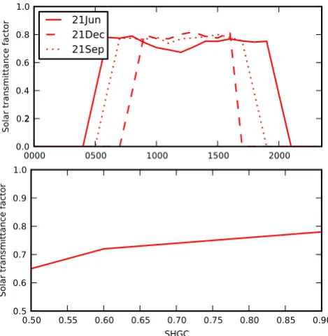
Fig. A1. Diurnal cycle of the solar transmittance factor of a
win-dow with a SHGC = 0.8 (top) and daytime-average solar transmit-tance factor for different SHGC (bottom). The solar transmittransmit-tance factor is defined as the ratio between the average of the solar trans-mittances for different window orientations and the SHGC. In the first graph, three characteristic days of the year are represented, the two solstices and an equinox.
Fm−wi=Fwi−mAwi/Am, (A12)
Fm−win=Fwin−mAwin/Am, (A13)
and
Fm−fl=Ffl−m/Am, (A14)
where the subscripts fl, m, wi, and win represent floor, in-ternal mass, inin-ternal wall, and window, respectively; GR is the glazing ratio of the building; and(h/w)fl represents the
aspect ratio of one building level. A1 Solar heat transmission
Generally, the solar heat transmitted through windows de-pends on the angle of incidence of the sun. However, based on simulations with EnergyPlus, we can show that the so-lar transmittance is proportional to the window SHGC for an average-oriented canyon. The Solar Transmittance Factor (STF) is defined as the ratio between the average of the so-lar transmittances for different window orientations and the SHGC.
A series of simulations were carried out with EnergyPlus for eight different orientations of a window in intervals of 45◦. Three characteristic days in Toulouse, the two solstices
and an equinox, were simulated for different values of the SHGC. Fig. A1a represents the diurnal cycle of STF for win-dows with a SHGC = 0.8. Fig. A1b shows the dependence of the daytime STF on the SHGC. From this analysis, we con-clude that a constant STF of 0.75±0.03 can be considered for an average-oriented window with a SHGC between 0.6 and 0.9.
A2 Natural ventilation
The natural ventilation module first compares indoor and out-door air temperatures. IfTin> Turb+1 K, the modules
esti-mates a natural ventilation potential, by calculating the in-door air temperature with and without natural ventilation, TopenandTclose, respectively.
The conditions are considered favourable for natural ventilation if Topen< Tcool,target,Topen< Tclose, and Topen>
Theat,target+4 K.
The natural ventilation air flowrate per unit width (V˙nv) is
calculated from the following equation for a single opening with bidirectional flow (Truong, 2012):
˙
Vnv=
1 3
gTin−Turb Tin
1/2
(A15)
hwin+
Tin
g (Tin−Turb)
1 2U
2 ref1Cp
3/2
wherehwinis the window height,1Cpis the pressure
coeffi-cient difference between the windward and the leeward sides of the building, andUrefis the average air velocity where the
pressure coefficients are measured. A3 Cooling system
BEM accounts for the dependence of a cooling system on outdoor and indoor conditions, through the definition of char-acteristic performance curves (DOE, 2010). The total cool-ing capacity is calculated from the rated capacity, modified by the following curve:
ϕQ=A1+B1Twb,i+C1Twb2,i+D1Tc,i+E1Tc2,i+F1Twb,iTc,i, (A16) whereTwb,i (◦C) is the wet-bulb temperature of the air
en-tering the cooling coil andTc,i (◦C) is the dry-bulb outdoor
air temperature, in an air-cooled condenser (wet-bulb out-door air temperature in an evaporative condenser). The ac-tual COP of the system is calculated from the nominal COP, divided by the following curve:
ϕCOP=A2+B2Twb,i+C2Twb2,i+D2Tc,i+E2Tc2,i+F2Twb,iTc,i. (A17) The coefficients used in Eqs. (A16) and (A17) are the de-fault ones used by EnergyPlus when a single-speed direct-expansion cooling system is defined: A1=0.942587793,
B1=0.009543347,C1=0.00068377,D1= −0.011042676,
E1=0.000005249,F1= −0.00000972,A2=0.342414409,
B2=0.034885008, C2= −0.0006237, D2=0.004977216,
The coefficientfPLRof Eq. (11) is given by:
fPLR=0.85+0.15PLR, (A18)
where PLR is the part-load ratio, calculated as the fraction between the energy supplied and the system capacity. A4 Autosize function
The rated cooling capacity is calculated by dynamically sim-ulating the building with predefined diurnal cycles of outdoor air temperature and incoming solar radiation. The diurnal cy-cle of outdoor air temperature has a maximum defined by the user and an amplitude of 10.7 K. The evolution is sinusoidal according to the following equation:
Tcan=Tsize,max−5.35+5.35sin(2π (t+57600)/86400). (A19) The solar radiation at each time step is given by:
S↓=KsolDcorrcos(Z), (A20)
where Ksol= 1367 W m−2, Dcorr = 1 + 0.0334cos
0.01721Djulian−0.0552, and Z is the solar zenith
angle; and whereDjulianis the Julian day of the year.
Acknowledgements. This study has received funding from the French National Research Agency under the MUSCADE project referenced as ANR-09-VILL-003, from the European Community’s Seventh Framework Programme (FP7/2007–2013) under grant agreement no. 211345 (BRIDGE Project). It has also been partially funded by the Singapore National Research Foundation through the Singapore-MIT Alliance for Research and Technology (SMART) Centre for Environmental Sensing and Modelling (CENSAM). We would also like to thank Synnefa from NKUA for providing the data for the Egaleo case study.
Edited by: S. Easterbrook
The publication of this article is financed by CNRS-INSU.
References
Adnot, J.: Energy Efficiency and Certification of Central Air Con-ditioners (EECCAC), ARMINES, Paris, France, 2003.
Bueno, B., Norford, L., Pigeon, G., and Britter, R.: Combining a detailed building energy model with a physically-based urban canopy model, Bound.-Lay. Meteorol., 140, 471–489, 2011. Bueno, B., Norford, L., Pigeon, G., and Britter, R.: A
resistance-capacitance network model for the analysis of the interactions between the energy performance of buildings and the urban cli-mate, Build. Environ., 54, 116–125, 2012.
Crawley, D. B., Lawrie, L. K., Winkelmann, F. C., Buhl, W. F., Huang, Y. J., Pedersen, C. O., Strand, R. K., Liesen, R. J., Fisher, D. E., Witte, M. J., and Glazer, J.: EnergyPlus: creating a new-generation building energy simulation program, Energy Build., 33, 319–331, 2001.
de Munck, C., Pigeon, G., Masson, V., Meunier, F., Bousquet, P., Trmac, B., Merchat, M., Poeuf, P., and Marchadier, C.: How much can air conditioning increase air temperatures for a city like Paris, France, Int. J. Climatol., doi:10.1002/joc.3415, 2012. DOE: EnergyPlus Engineering Reference, EnergyPlus, 2010. Grimmond, C. S. B., Blackett, M., Best, M. J., Baik, J.-J., Belcher,
S. E., Beringer, J., Bohnenstengel, S. I., Calmet, I., Chen, F., Coutts, A., Dandou, A., Fortuniak, K., Gouvea, M. L., Hamdi, R., Hendry, M., Kanda, M., Kawai, T., Kawamoto, Y., Kondo, H., Krayenhoff, E. S., Lee, S.-H., Loridan, T., Martilli, A., Masson, V., Miao, S., Oleson, K., Ooka, R., Pigeon, G., Porson, A., Ryu, Y.-H., Salamanca, F., Steeneveld, G., Tombrou, M., Voogt, J. A., Young, D. T., and Zhang, N.: Initial results from Phase 2 of the international urban energy balance model comparison, Int. J. Climatol., 31 , 244–272, 2011.
Hamdi, R. V., and Masson, V.: Inclusion of a drag approach in the Town Energy Balance (TEB) Scheme: Offline 1-D validation in a street canyon, J. Appl. Meteorol. Climatol., 47, 2627–2644, 2008.
Ihara, T., Kikegawa, Y., Asahi, K., Genchi, Y., and Kondo, H.: Changes in year-round air temperature and annual energy con-sumption in office building areas by urban heat-island counter-measures and energy-saving counter-measures, Appl. Energy, 85, 12–25, 2008.
Kikegawa, Y., Genchi, Y., Yoshikado, H., and Kondo, H.: Devel-opment of a numerical simulation system for comprehensive as-sessments of urban warming countermeasures including their im-pacts upon the urban building’s energy-demands, Appl. Energy, 76, 449–66, 2003.
Kikegawa, Y., Genchi, Y., Kondo, H., and Hanaki, K.: Im-pacts of city-block-scale countermeasures against urban heat-island phenomena upon a building’s energy-consumption for air-conditioning, Appl. Energy, 83, 649–668, 2006.
Kondo, H. and Kikegawa, Y.: Temperature variation in the urban canopy with anthropogenic energy use, Pure Appl. Geophys., 160, 317–324, 2003.
Lemonsu, A., Grimmond, C. S. B., and Masson, V.: Modelling the surface energy balance of the core of an old Mediterranean city: Marseille, J. Appl. Meteorol., 43, 312–327, 2004.
Lemonsu, A., B´elair, S., Mailhot, J., and Leroyer, S.: Evaluation of the Town Energy Balance Model in Cold and Snowy Conditions during the Montreal Urban Snow Experiment 2005, J. Appl. Me-teorol. Climatol., 49, 346–362, 2010.
Masson, V.: A physically-based scheme for the urban energy bud-get in atmospheric models, Bound.-Lay. Meteorol., 94, 357–397, 2000.
Masson, V., Grimmond, C. S. B., and Oke, T. R.: Evaluation of the Town Energy Balance (TEB) scheme with direct measurements from dry districts in two cities, J. Appl. Meteorol., 41, 1011– 1026, 2002.
Interactions in Toulouse Urban Layer (CAPITOUL) experiment, Meteorol. Atmos. Phys., 102, 135–157, 2008.
Offerle, B., Grimmond, C. S. B., and Fortuniak, K.: Heat storage and anthropogenic heat flux in relation to the energy balance of a central European city centre, Int. J. Climatol., 25, 1405–1419, 2005.
Oke, T. R.: The urban energy balance, Prog. Phys. Geogr., 12, 471– 508, 1988.
Pigeon, G., Legain, D., Durand, P., and Masson, V.: Anthropogenic heat release in an old European agglomeration (Toulouse, France), Int. J. Climatol., 27, 1969–1981, 2007.
Pigeon, G., Moscicki, A. M., Voogt, J. A., and Masson, V.: Sim-ulation of fall and winter surface energy balance over a dense urban area using the TEB scheme, Meteorol. Atmos. Phys., 102, 159–171, 2008.
Salamanca, F. and Martilli, A.: A new building energy model cou-pled with an urban canopy parameterization for urban climate simulations, Part II. Validation with one dimension off-line sim-ulations, Theor. Appl. Climatol., 99, 345–356, 2010.
Salamanca, F., Krpo, A., Martilli, A., and Clappier, A.: A new Building Energy Model coupled with an Urban Canopy Param-eterization for urban climate simulations, Part I. Formulation, verification and a sensitive analysis of the model, Theor. Appl. Climatol., 99, 331–344, 2010.
Synnefa, A., Stathopoulou, M., Sakka, A., Katsiabani, K., Santa-mouris, M., Adaktylou, N., Cartalis, C., and Chrysoulakis, N.: Integrating sustainability aspects in urban planning: the case of Athens, 3rd International Conference on Passive and Low En-ergy Cooling for the Built Environment (PALENC 2010) & 5th European Conference on Energy Performance & Indoor Climate in Buildings (EPIC 2010) & 1st Cool Roofs Conference, Rhodes Island, Greece, 29 September–1 October 2010.