Tracking of coherent thermal structures on a heated wall.

Tracking of coherent thermal structures on a heated wall.

2. DNS simulation

T.A. Kowalewski, A. Mosyak, G. Hetsroni

Abstract The temporal evolution of a thermal pattern observed on a heated wall by infrared camera is correlated with the propagation velocity of the thermal perturbations calculated by DNS. In the experiment the propagation velocity was measured by using PIV-based analysis of in-frared images of the thermal pattern on the wall. To verify the experimental technique of image analysis, a sequence of synthetic images, simulating thermal patterns on the wall, was generated from the DNS solution, and the convective velocity was evaluated. It was found that the convective velocity of thermal structures obtained by PIV-based analysis of the experimental and synthetic images was in relatively good agreement with that calculated from the DNS solution. The present study confirmed that for a high Prandtl number fluid (water) the propagation velocity of the thermal perturbations is only about half of the convective velocity of the velocity perturbations. It was also found that the convection velocity observed for hot spots is distinctly lower than that for the cold spots.

1

Introduction

Turbulent flow structures are strongly influenced by in-teractions between the flow and the wall. Many studies have been devoted to the experimental investigation of this problem. Observed fluctuations of the flow indicate very distinct intermittency of the turbulent flow close to the

boundary. It appears that particular quasi-periodic bursting structures can be identified in the wall layers. These events, of relatively short duration and pro-nounced turbulence activity, during which most of the turbulent energy is generated, consist of at least two phases: ejections of low-momentum fluid masses from the near-wall region, and injections of high-momentum fluid masses toward the wall. The ejections and the injections occur intermittently, and in interaction with the flow they produce high instantaneous fluctuations of the local heat or mass transfer at the wall. These fluctu-ations can be visualized by recording the instantaneous temperature fields at the wall (Kaftori et al. 1994; Hetsroni and Rozenblit 1994; Hetsroni et al. 1996; Irtani et al. 1983).

The correlation between the spatial characteristic of the thermal field and that of the velocity is an important issue of turbulence studies (Krogstad et al. 1998; Kawamura et al. 1998, 1999). If the temperature differ-ences within the boundary layer are small, the buoyancy effects can be neglected. In such cases the thermal pattern convected by the flow may be considered as a passive scalar (Herman et al. 1998). Hence, nonintrusive measurements of instantaneous thermal fields within the flow and at the walls can deliver valuable information about turbulent characteristics of the flow. However, it is important to note that the passive scalar behavior can be strongly modified if local isotropy is violated (Warhaft 2000). It seems to be necessary to find proper relations between momentum and heat transport for turbulent flow. Therefore understanding the behavior of passive scalars is a challenging new problem of great practical importance. One possible method to visualize the pres-ence of thermal structures is thermography, which makes it possible to acquire the information about the struc-tures directly at the wall without introducing any flow perturbation. This is a very important issue, as the use of most of the available flow analysis methods, such as la-ser-Doppler anemometry, particle image velocimetry (PIV), or hot-wire techniques, is limited to large nondi-mensional distances from the wall. A key question is whether the wall temperature measurements reflect the scaling and response times of organized hydrodynamic structures.

In our previous paper (Hetsroni et al. 2001) it was shown that a relatively simple analysis of the thermal fluctuations observed on the wall could be used to obtain turbulent characteristics of the underlying fluid flow. The proposed method may be attractive in many practical Experiments in Fluids 34 (2003) 390–396

DOI 10.1007/s00348-002-0574-9

390

Received: 27 May 2002 / Accepted: 11 November 2002 Published online: 9 January 2003

Springer-Verlag 2003

T.A. Kowalewski (&)

IPPT PAN, Polish Academy of Sciences, Swietokrzyska 21,

PL 00–049 Warszawa, Poland

E-mail: [email protected] Fax: +48-22-8269803

A. Mosyak, G. Hetsroni

Department of Mechanical Engineering, Technion IIT, 32000, Haifa, Israel

applications as it allows for the analysis of turbulence without any optical or mechanical access to the flow.

In the present paper data available from the direct numerical simulation (DNS) of the flow are used to verify and refine the conclusions obtained on the convective velocity of the thermal structures and to confirm observed difference between the convection velocity of ‘‘hot spots’’ and ‘‘cold spots’’. In the following it is shown that the thermal fluctuations observed on the wall in the experi-ment actually correspond to the convective thermal structures identified within the bulk flow generated for a similar flow using direct numerical simulation.

2

Formulation of the problem

We consider the experimental configuration described in Hetsroni et al. (2001). It consists of an open flume (4.3-m long, 0.32-m wide and 0.1-m deep) with a pump that forces circulation of constant-temperature water. The flow depth is 0.037 m, and the hydraulic diameter is 0.066 m. The water temperature at the inlet is 20C±0.1C. A fully de-veloped turbulent flow is established in the region beyond 2.5 m downstream from the inlet of the flume. At this distance a 170·135-mm patch made of 50-lm thick con-stantan foil is mounted at the bottom of the flume. The foil is heated by DC current to produce a constant heat flux

q=12 kWm)2. Temperature variations in the range of 2C are observed on the foil by an infrared (IR) radiometer. For small temperature variations the imposed buoyancy effects are negligible and the temperature field behaves as a passive scalar. Hence, the temperature distribution on the wall can be considered as a trace of the flow structure near the bottom wall.

The measured value of average streamwise water ve-locity wasU0=0.25 m/s, and the corresponding Reynolds number based on the water height wasRe=9200. The experimental value of shear velocityu*=0.0133 m/s agrees well with thelogarithmic law of the wall:

U+=2.5ln(x3+)+5.0. Throughout this paper the streamwise direction is denoted byx1, the spanwise direction byx2, and the wall-normal direction byx3, while the velocity components areu1, u2,u3, correspondingly. Quantities

UandVdenote the mean local flow velocity and the perturbation velocity in the streamwise direction, respec-tively. Velocity, time, and distance are normalized by wall units asui+=ui/u*,t+=tu*2/v, and xi+=xiu*/v, where v denotes the kinematic viscosity of fluid.

The above experimental configuration was investigated using the direct numerical simulation (DNS) technique described in detail by Tiselj et al. (2001). However, it should be noted that because of computational constraints the present DNS was performed at a lower Reynolds number, i.e. atRe=2600.

3

Experiment

Because the experiment is described in detail elsewhere (Hetsroni et al. 2001), here we repeat only the main con-siderations. The experimental setup consisted of an in-frared scanner, an S-VHS video recorder, a computer, a monitor and an 8-bit frame grabber. The radiometer was

located at a distance of 0.5 m, and the IR image created on the foil was recorded from below. The frequency response of heated foil used in the present experiments is 0.04 s, which is short enough to investigate convection velocity of the thermal perturbations generated on the wall (Hetsroni et al. 2001).

The image analysis used to determine the convective velocity of a thermal pattern was based on the two-di-mensional correlation between thermal patterns found within the analyzed images. It was preformed applying the well-known PIV approach to IR images. The high-resolu-tion method (Quenot et al. 1998) used allowed us to evaluate convective velocity of the thermal spots at each pixel of the IR image.

The high and low temperature streaks, clearly seen on the wall surface, indicate the presence of coherent struc-tures advected by the main flow (cf. Fig. 6 in Hetsroni et al. 2001). Looking at a longer sequence of images it appears that the dark (cold) patches move faster and often over-take adjacent bright (hot) streaks. The high and low temperature streaks may also interact with each other.

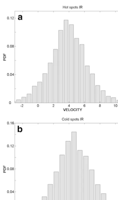
By evaluating bright and dark spots separately it was found that the hot and cold structures have different convective velocities. Remembering that the wall temper-ature strongly depends on the third velocity component (from or to the wall), this difference in the convective velocity can be used to determine different coherent structures acting on the wall. Figure 1 shows velocity histograms obtained for the sequence of 16 images eval-uated separately for hot and cold thermal spots. Looking at the velocity histogram (Fig. 1), we may note that the measured streamwise velocity is characterized by a very broad spectrum with a flat maximum close toVT+=4 for the hot spots and a slightly higher value for the cold spots. By taking the time and space average for the whole se-quence, the mean velocity obtained for hot spots is equal toVT+=3.76, and for the cold spots isVT+=4.77. We hy-pothesize that these values correspond to the mean propagation velocity of coherent flow structures respon-sible for the ejection bursts from the wall (positive temperature pulse) and for the injections of the fluid to the wall (negative temperature pulse, cf. Krogstad et al. 1998).

To verify this assumption it is necessary to correlate the results obtained from the analysis of thermal images with the corresponding flow structure within the channel. Experimentally, such a procedure is difficult to perform. The main reason is the difficulty in obtaining acceptable velocity and temperature measurements for small dis-tances from the wall (x3+<10). Hence, we looked for the corresponding data obtained from DNS of the fully developed turbulent flow in an open channel.

4

DNS method and determination of convection velocity

The DNS solution obtained for a fully developed turbulent flow atPr=0.71 andPr=5.4 in an open channel was used to analyze the convection velocity of thermal perturbations. Details of the numerical method and the turbulent data analysis are described by Tiselj et al. (2001) in a separate paper, and here we only repeat its main points.

The time-dependent three-dimensional Navier–Stokes and continuity equations were solved in a rectangular domain. The flow geometry and coordinate system are shown in Fig. 2. The flow is driven by a constant stream-wise pressure gradient. The boundary conditions are no slip on the bottom wall, and free slip on the free surface. Periodic boundary conditions are imposed in the stream-wise (x1) and spanwise (x2) directions.

In the numerical code a pseudo-spectral method is employed to solve the governing equations. In the ho-mogeneous directions (x1andx2), all the quantities are

expressed by Fourier expansions. In thex3-direction, which is nonhomogeneous, the quantities are represented by Chebyshev polynomials. A full description of the nu-merical scheme can be found in Lam (1989). In the present numerical study, the bulk Reynolds number is 2600 (the turbulent Reynolds number used in the simulations is

Re*=85.4). The calculations were carried out in a com-putational domain ofL1+·L2+·L3+=1074·537·171 wall units in thex1-,x2- andx3-directions with a resolution of 128·128·65. This resolution was selected as a compromise between accuracy and computational time. It was found that the use of larger computational volumes does not produce significant changes of the turbulence statistics (Tiselj et al. 2001). A nonuniform distribution of colloca-tion points is used in thex3-direction due to the nature of the Chebyshev polynomials, and the first collocation point away from the wall is atx3+=0.1.

It is assumed that all fluid properties are constant, and the buoyancy is neglected. As the initial condition a uni-form distributed temperature field was projected on the velocity field. The heat transfer simulation was started after the velocity field reached a steady state. Then once the velocity field was calculated at each time step, the temperature field was obtained by integrating the energy equation with the same grid system used for the velocity field. Two different thermal boundary conditions were considered: assuming isothermal wall (Tw=const.) and constant heat flux (qw=const.). The last assumption cor-responds to our experimental case.

The effect of the wall boundary condition on scalar transfer in a fully developed turbulent flume was studied by Tiselj at al. (2001). It was found that the type of thermal boundary conditions has a profound affect on the statistics of the temperature fluctuations in the near-wall region (x3+<10). For low Prandtl numbers (Pr=1), the turbulent boundary layer significantly influences the scalar transfer in the conductive sublayer; whereas at higher Prandtl numbers (Pr=5.4) the near-wall temperature field may be associated with predominant motion in the viscous sub-layer. It effectively influences convective velocities of thermal fluctuations in the near-wall region.

Tiselj at al. (2001) gave a detailed discussion on the code reliability. Hence, we use numerical fields generated with this code to the present analysis. For this purpose, sequences of about 50 instantaneous velocity and tem-perature fields taken at a regular time interval (Dt+=2.416) were stored after solution for the temperature field reached the statistical steady state.

The streamwise component of convection velocity of thermal perturbation is determined by streamwise space– time correlation, i.e.Dx2=Dx3=0. There are several ways to determine convection velocity. Here we consider the signal convection velocity of temperature perturbations, follow-ing Kim and Hussain (1993), who investigated the signal convection velocity of velocity, pressure, and vorticity perturbations. The signal velocity is the velocity with which the main portion of the signal amplitude travels. It can be measured by the location of the peak of space–time cross-correlation in an instantaneous field. The convection velocities of temperature fluctuations along the channel are shown in Fig. 3 for two thermal boundary conditions:

Fig. 2.Computational domain, coordinate system and thermal

wall boundary conditions

Fig. 1a,b. Experimental results. Histograms of nondimensional

streamwise velocity evaluated for a sequence of IR images.a, hot spots evaluation, mean velocityVT+=3.76;b, cold spots evaluation, mean velocityVT+=4.77

constant heat flux and for the isothermal wall. For parison, the mean flow velocity and the streamwise com-ponent of convection velocity of velocity perturbation (VU1+) are plotted.

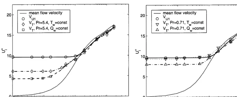
It is worth noting that for most of the outer part of the channel, sayx3+>20, the convection velocities for the ve-locity perturbations are almost identical with the local mean flow velocityU. Near the wall, however, all convec-tion velocities for perturbaconvec-tions exceedU, becoming constant forx3+ <10. It can also be seen that close to the wall (x3+<10) the convection velocities for temperature and velocity perturbations are different, and that the ve-locity of the temperature perturbations depends on the thermal boundary conditions imposed on the wall. In Fig. 3 we may see that at the bottom wall (x3+=0) the convective velocity ofVT+for the constant wall heat flux boundary condition is only 4.33, while for the isothermal wall it is 5.33, which is well below the convection velocity of velocity perturbations (approximately 10 in the wall region). For comparison, Fig. 4 shows the propagation velocity of the thermal perturbations for low Prandtl number flow (Pr=0.71). In this case the propagation ve-locities are significantly higher.

Our experimental visualization indicates the existence of thermal structures that propagate streamwise, which are evident as appearing or disappearing hot and cold spots. Their existence is related to the local bursts transporting fluid from or to the wall. These are known to travel for considerable streamwise distances without losing their identity (Hetsroni et al. 1997, 1999) and should therefore provide reliable information about the convection veloci-ties. Hence, to identify them it should be more efficient to derive convection velocities from detection of typical thermal signatures. In order to address this problem, the convection velocity of strong temperature discontinuities on the bottom wall was studied. For this purpose, an

adaptation of the window average gradient (WAG) algo-rithm was used (Bisset et al. 1991). The WAG algoalgo-rithm was developed to search for large-scale events by focusing on rapid transitions in the signal. The modified detection function is defined as

Sign T t½ ð0þDtÞ T tð Þ0 kTrms; ð1Þ

whereTrepresents the temperature, andkis the threshold parameter. The thermal fields were evaluated at a time intervalDt+=19.328, which was found to be the best time interval to determine the convection velocity by the space– time correlation method. This time interval is also in agreement with the window length (Dt+=20) used by Krogstad et al. (1998). IfSignis taken to be +1, detection triggers on the rapid transition from low to high values of temperature. Perhaps this is characteristic of the transition from the end of a sweep to the beginning of an ejection. Conversely, forSign=–1, the detection points may represent the end of an ejection and the onset of a sweep.

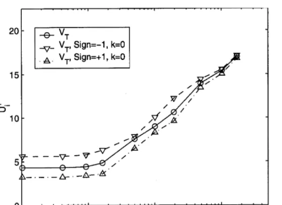
For the threshold parameterk=0, the whole thermal field is divided into two parts with increasing and decreasing temperature. The convection velocities of these two parts are shown in Fig. 5 across the channel depth. It can be seen that the convection velocities for decreasing temperature (Sign=–1) are always faster than those for increasing tem-perature (Sign=+1) in the whole depth, and this effect is much pronounced in the near-wall region. The convection velocity of the temperature fluctuations obtained from the space–time correlations VTfalls in the limits between VT+1 and VT)1. This result corroborates with the observations by Krogstad and Antonia (1994) of the streamwise pattern near large-scale positive discontinuities and agrees with the results of Krogstad et al. (1998), where the convection velocity of velocity discontinuities was measured.

In Fig. 5 we see that at the near-wall region the con-vective velocity VTþ obtained for the constant heat flux

boundary conditions is 5.60 for the negative (cold)

tran-Fig. 4.DNS solution. Convection velocities of temperature

perturbations across the channel depth for low Prandtl number flow (Pr=0.7)

Fig. 3. DNS solution. Convection velocities of thermal

disconti-nuitiesVTacross the channel depth calculated for water flow (Pr=5.4) under the isothermal wall and constant wall heat flux boundary conditions compared with the mean flow velocity profile (solid line) and convection velocity of velocity perturba-tionsVU1

sition, and only 3.24 for the positive (hot) transition. It is worth noting that these values are qualitatively in a good agreement with our experimental findings reported in Sect. 3 for the convective velocity of the hot and cold thermal structures (dark and bright spots). However, there is still an open question whether the displacements eval-uated in the physical experiment from the thermal images are good representatives of the convective velocity of the thermal coherent structures visualized on the other side of the wall. To elucidate this problem, a sequence of synthetic images simulating thermal patterns at the wall was gen-erated from the DNS solution. These images were analyzed in the same way as the physical images from the IR sensor.

5

Image analysis of synthetic thermal images

The essential streak formation mechanism of near-wall coherent flow structures is the localized lift-up of low-speed fluid near the wall by advecting streamwise vortices. Our image analysis of the thermal streaks indicates that their propagation velocity is close to that obtained in the numerical simulations for the convection velocity of the thermal structures. However, in our method of analysis an arbitrary selection of the threshold for hot/cold spots as well as the PIV-based image-processing procedure may introduce an unknown bias to the results obtained. Hence, we now address the question whether the behavior of the observed thermal ‘‘fingerprints’’ describes the underlying flow characteristics well enough. For this purpose, the temperature field calculated on the wall is used to generate gray-level contours simulating the IR images. Figure 6 shows isotherms calculated for the wall displayed as 64 gray levels expanded to the full 8-bit intensity range (0–255). These synthetic images of the wall temperature show longitudinal structures similar to these observed in the experiment (Hetsroni et al. 2001). By applying the PIV evaluation procedure (Sect. 3) to these images the con-vective velocity of the simulated thermal spots is found.

To compare this evaluation with our experimental data, a sequence of 31 images simulating IR maps was generated for water flow using the DNS simulation described in Sect. 4. Three different time intervals between images were used:Dt+=2.416, 4.832 and 9.644. It was found that the most appropriate time interval for PIV analysis of the synthetic images was 4.832, close to that found for the experimental data.

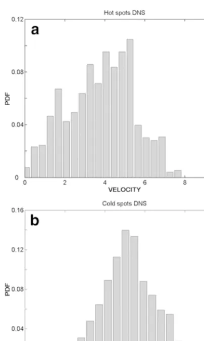
For each sequence of images, the time and space average of the longitudinal convective velocity of ‘‘ther-mal’’ streaks was calculated, separately for hot and cold regions. Figure 7 shows histograms for the streamwise velocity obtained in this way for a sequence of the syn-thetic images. We note several similarities to Fig. 1, which shows the experimental data. The evaluated con-vective velocity is characterized by a rather broad dis-tribution, especially for the hot spots. This may be due to the rather low resolution of the synthetic images, de-grading our PIV analysis. Nevertheless, we may clearly distinguish a difference in the mean velocity of the cold and hot spots. The mean values of convective velocity VTþ calculated for the whole sequence was found to be

4.44 for the cold spots, and 3.78 for the hot spots. Table 1 collects the results of our two evaluations of convective velocities obtained from the experimental (PIV–EXP) and synthetic images (PIV–DNS). It is interesting to note that convective velocities obtained from the synthetic images are very close to our experimental averages, i.e. 4.77 and 3.76, respectively. Despite an over three-fold difference in the Reynolds number, our physical and synthetic thermal streaks exhibit very similar behavior. This confirms that our optical evaluation method works correctly for both the experimental and synthetic images. For both cases, we also have qualitative agreement with the convective velocity of the thermal signatures, (DNS row in Table 1). However, quantitatively they differ by more than 10% from the directly calculated convective velocities of the thermal discontinuities, particularly for velocities of the cold spots. It is obvious that our PIV method of analysis cannot exactly reproduce these values, as the analyzed thermal streaks are already objects that represent spatial temperature averages. Nevertheless, their correlation with the thermal signatures defined for the DNS data is evi-dent.

Some differences in the statistical characteristics of the evaluated convective velocities, already visible in the his-tograms, are described by the standard deviation,

skew-Fig. 6.Synthetic image of the wall temperature field generated

from the DNS solution for water (Pr=5.4)

Fig. 5.DNS solution. Convection velocity of temperature

ness, and flatness in Table 1. Generally, the experimental data show broader scatter, which is rather obvious. The evaluated distribution of convective velocity for both ex-perimental and synthetic images, as well as DNS data, shows rather weak asymmetry (skewness about ±0.2). It may confirm that temperature fluctuations for high Prandtl numbers are greatly damped by molecular diffu-sion in the wall region, as described by Na and Hanratty (2000). This affects the convective velocities of the thermal perturbations and is responsible for the observed

dissimilarities between momentum and heat transport in a turbulent boundary layer (Kong et al. 2001).

6

Discussion

Examination of the near-wall turbulence characteristics is essential for predicting heat and mass transfer between a solid boundary and a turbulent flow. Hence, over the last 20 years a large number of experimental, theoretical, and numerical investigations were devoted to elucidate the impact of energy transfer rate fluctuations at the near-wall region upon the global statistical properties of turbulence. It is worthwhile to summarize the main points of the knowledge gathered to date.

Kim and Hussain (1992) found that in the wall region (x3+<10) the propagation velocity of velocity fluctuations remains almost constant, approaching a limiting value of about 10 wall units, i.e. 0.55 of the main stream velocity. The near-wall turbulence consists of at least two phases: ejections of low-momentum fluid masses from the wall vicinity, and injections of high-momentum fluid masses toward the wall. It produces the highly non-Gaussian probability distribution of the statistical characteristics. It is pronounced in slight differences of the convection ve-locities for ejections and injections, as shown by Krogstad et al. (1998).

One of the main properties inferred from recent in-vestigations is the dissimilarity between the velocity and scalar transport close to a wall. The problem is discussed in numerous papers and found in an excellent review by Warhaft (2000). The behavior of passive scalars described by temperature or concentration fluctuations may exhibit different statistics than velocity, especially for high mo-lecular Prandtl or Schmidt numbers. For their values close to unity and for the same type of boundary conditions as for the velocity, the near-wall transport characteristics of the passive scalars quite closely follow that for the velocity fluctuations (Kawamura et al. 1998; Calmet and Magnau-det 1997). Therefore for low Prandtl number fluids (air), the temperature fluctuations observed at the isothermal wall are directly related to the convection velocity of ve-locity fluctuations. Dissimilarities in the temperature and velocity fluctuations are apparent for the isoflux boundary conditions (Tiselj et al. 2001). For isothermal boundary conditions the thermal field in the near-wall region is al-most identical to the velocity field with profound asym-metry. In contrary, comparison of the streamwise velocity field and the temperature field at isoflux boundary con-ditions reveals significant differences. The skewness factor of thermal fluctuations remains close to zero all the way close to the wall. It seems that for the isoflux thermal boundary conditions, the near-wall temperature fluctua-tions modify the nature of scalar transfer from large to small scales. It affects the streamwise convective velocities of thermal fluctuations (Fig. 4).

At high Prandtl (or Schmidt) numbers the temperature (or concentration) field is unable to diffuse efficiently in the near-wall region and directly follows the inflows and outflows associated with the bursting events. The thermal sublayer is much thinner, and only very small turbulent structures are able to contribute to heat transfer. The

Fig. 7a,b. Histograms of nondimensional streamwise velocity of

the wall thermal structures evaluated for a sequence of ten synthetic images generated from the DNS solution,Dt+=4.832. a, hot spots evaluation, mean velocityVT+=3.78;b, cold spots evaluation, mean velocityVT+=4.44

Table 1.Evaluation of the meanconvective velocity of thermal

perturbations, standard deviation (Std),skewness (S) and flatness (F); image-processing–based velocityobtained for the

experimental IR images (PIV–EXP) and for thesynthetic images from DNS data (PIV–DNS). DNS values of convectivevelocity of velocity (VU) and temperature (VT) perturbations evaluated from the numerical fields

VU VTSign=–1 (cold spots)

VTSign=+1 (hot spots)

Mean Mean Std S F Mean Std S F

PIV–EXP – 4.77 2.34 0.11 2.94 3.76 2.33 –0.17 3.15 PIV–DNS – 4.44 1.35 0.21 2.92 3.78 1.35 0.25 2.91 DNS 10 5.60 – 0.14 2.75 3.24 – 0.14 2.75

dissimilarity between the velocity and temperature fluc-tuations atPr>1 leads to the observed dissimilarity in their convection velocity. It appears that the small-scale fluc-tuations in scalar fields are advected by turbulent flow at lower velocities, for isoflux as well as for isothermal boundary conditions (Fig. 3).

7

Conclusions

The present analysis confirmed the ability of the PIV-based evaluation method to track the coherent thermal structures visualized at the wall by an IR camera. Our preliminary study shows that the temporal and spatial analysis of long time sequences of thermal images can be used to evaluate the basic characteristics of the underlying fluid flow. It is shown that the mean convective velocity of coherent structures can be relatively well evaluated from the thermal pattern dynamics. It is worth noting that the method offers a unique opportunity to obtain basic flow characteristics without any optical or mechanical access to the flow. It may have great practical importance for studying turbulent transport in industrial installations.

Our analysis of the thermal structures observed at the wall confirms the DNS findings that under constant wall heat flux there is a general trend for the negative thermal discontinuities to be convected at somewhat higher ve-locities than the positive ones. Since the negative thermal discontinuities are mainly linked with the end of an ejec-tion and onset a sweep, and positive thermal discontinu-ities with the end of a sweep to the beginning of an ejection, it can be concluded that a high-speed fluid region followed by a low-speed region is convected at a higher speed than a low-speed fluid region followed by a region of higher velocity. This is qualitatively in agreement with observations by Krogstad et al. (1998), who found up to 20% difference of the convection velocity between sweeps and ejections for a wind tunnel flow.

Under the conditions of our experiment, the time-and space-averaged dimensionless value of propagation velocity of coherent thermal structures obtained for hot spots was VT+=3.76, and for the cold spots was

VT+=4.77. Very close values were obtained using the same method of analysis for the synthetic images gen-erated from a DNS of a similar flow. Our analysis of the DNS solution shows that the thermal discontinuities propagate at a velocity very close to that found from the image analysis of the thermal spots. Hence, we suppose that there is a strong correlation between the dynamics of the thermal structures observed on the wall and the momentum and heat transport in the turbulent bound-ary layer.

The DNS simulations allowed us to relate the propa-gation velocity of large-scale temperature structures to that of velocity perturbations. We confirmed the dissimi-larity between the streamwise velocity and temperature fields in the near-wall region. It appears that this relation is highly dependent on the molecular Prandtl number. For fluids characterized by higher Prandtl numbers, such as water used in the experiment, the convective velocity of coherent thermal structures is only about half of that for momentum transport. This is in general agreement with

findings of Na and Hanratty (2000), who obtained for

Pr=10 the convection velocity in the near-wall temperature fieldVT+3.9. For low Prandtl number fluids the differ-ence is smaller, and the convection velocity of thermal perturbation is about 90% of that for the velocity pertur-bations. This topic is certainly important, and the mo-mentum and heat transfer relations for the near-wall regions should be investigated in the future. Further studies seem necessary to obtain the proper relation for transport and mixing properties of the scalars for arbitrary Prandtl or Schmidt numbers.

References

Bisset DK, Antonia RA, Raupach MR (1991) Topology and transport properties of large-scale organized motion in a slightly heated rough wall boundary layer. Phys Fluids A 3:2220–2228

Calmet I, Magnaudet J (1997) Large-eddy simulation of high-Schmidt number mass transfer in a turbulent channel flow. Phys Fluids 9:438–455

Herman C, Kang E, Wetzel M (1998) Expanding the application of holographic interferometry to the quantitative visualization of oscillatory thermofluid process using temperature as tracer. Exp Fluids 24:431–436

Hetsroni G, Kowalewski TA, Hu B, Mosyak A (2001) Tracking of coherent thermal structures on a heated wall by means of IR thermography. Exp Fluids 30:286–294

Hetsroni G, Mosyak A, Rozenblit R, Yarin LP (1999) Thermal patterns on the smooth and rough walls in turbulent flows. Int J Heat Mass Transfer 42:3815–3829

Hetsroni G, Mosyak A, Yarin LP (1997) Thermal streaks regeneration in the wake of a disturbance in a turbulent boundary layer. Int J Heat Mass Transfer 40:4161–4168

Hetsroni G, Rozenblit R (1994) Heat transfer to a liquid solid mixture in a flume. Int J Multiphase Flow 20:671–689

Hetsroni G, Rozenblit R, Yarin LP (1996) A hot-foil infrared tech-nique for studying the temperature field of a wall. Meas Sci Technol 7:1418–1427

Iritani Y, Kasagi N, Hirata N (1983) Heat transfer mechanism and associated turbulence structure in the near wall region of a tur-bulent boundary layer. In: Fourth Symposium on Turtur-bulent Shear Flows, Karlsruhe, Germany, 12–14 September, pp 17.31–17.36 Kaftori D, Hetsroni G, Banerjee S (1994) Funnel-shaped vortical

structures in wall turbulence. Phys Fluids 6:3035–3050

Kawamura H, Abe H, Matsuo Y (1999) DNS of turbulent heat transfer in channel flow with respect to Reynolds and Prandtl number effects. Int J Heat Fluid Flow 20:196–207

Kawamura H, Ohsaka K, Abe H, Yamamoto K (1998) DNS of tur-bulent heat transfer in channel flow with low to medium-high Prandtl number fluid. Int J Heat Fluid Flow 19:482–491 Kim J, Hussain F (1993) Propagation velocity of perturbations in

turbulent channel flow. Phys Fluids 5:695–706

Kong H, Coi H, Lee JS (2001) Dissimilarity between the velocity and temperature fields in a perturbed turbulent thermal layer. Phys Fluids 13:1466–1479

Krogstad PA, Antonia RA (1994) Structure of turbulent boundary layers on smooth and rough walls. J Fluid Mech. 277:1–21 Krogstad PA, Kaspersen JH, Rimestad S (1998) Convection velocities

in turbulent boundary layers. Phys Fluids 10 :949–957

Lam KK (1989) Numerical investigation of turbulent flow bounded by a wall and a free-slip surface. PhD thesis, Univ of California, Santa Barbara

Na Y, Hanaratty TJ (2000) Limiting behavior of turbulent transport close to a wall. Int J Heat Mass Transfer 43:1749–1758

Quenot GM, Pakleza JM, Kowalewski TA (1998) Particle image ve-locimetry with optical flow. Exp Fluids 25:177–189

Tiselj I, Pogrebnyak E, Li C, Mosyak A, Hetsroni G (2001) Effect of wall boundary condition on scalar transfer in a fully developed turbulent flume. Phys Fluids 13:1028–1039

Warhaft Z (2000) Passive scalars in turbulent flows. Annu Rev Fluid Mech 32:203–240