in the population sciences published by the Max Planck Institute for Demographic Research Konrad-Zuse Str. 1, D-18057 Rostock·GERMANY www.demographic-research.org
DEMOGRAPHIC RESEARCH
VOLUME 19, ARTICLE 30, PAGES 1179-1204
PUBLISHED 08 JULY 2008
http://www.demographic-research.org/Volumes/Vol19/30/ DOI: 10.4054/DemRes.2008.19.30
Research Article
The modal age at death and the shifting
mortality hypothesis
Vladimir Canudas-Romo
c
°2008 Canudas-Romo.
1 Introduction 1180
2 Modal age 1181
3 Mortality models 1183
3.1 Gompertz mortality change model 1184
3.2 Logistic model 1186
3.3 Siler mortality change model 1189
3.3.1 Siler model 1189
3.3.2 Log-Siler model 1190
4 Concentration of the number of deaths around the modal age at death 1193
5 Six industrialized countries: An illustration 1194
6 Discussion 1195
7 Conclusion 1197
8 Acknowledgements 1199
References 1200
The modal age at death and the shifting mortality hypothesis
Vladimir Canudas-Romo1
Abstract
The modal age at death is used to study the shifting mortality scenario experienced by low mortality countries. The relations of the life table functions at the modal age are ana-lyzed using mortality models. In the models the modal age increases over time, but there is an asymptotic approximation towards a constant number of deaths and standard devia-tion from the mode. The findings are compared to changes observed in populadevia-tions with historical mortality data. As shown here the shifting mortality scenario is a process that might be expected if the current mortality changes maintain their pace. By focusing on the modal age at death, a new perspective on the analysis of human longevity is revealed.
1Department of Population, Family & Reproductive Health, Johns Hopkins Bloomberg School of Public
1. Introduction
Lexis (1878) considered that the distribution of deaths consisted of three parts: a decrease in the high number of deaths with age after birth to account for infant mortality; deaths centred around the late modal age at death (referred to hereafter as modal age at death), accounting for senescent mortality; and premature deaths that occur infrequently at young ages between the high infant mortality and senescent deaths. Life expectancy, or the mean of the life table distribution of deaths, is the indicator most frequently used to describe this distribution. In a regime with a high level of infant mortality, life expectancy will be within the age range of premature deaths, even when most deaths occur around ages zero and the modal age at death. The early stages of the epidemiological transition (Omran 1971) are characterized by a reduction in infant mortality. These changes in infant mor-tality have been captured very accurately with the rapid increase in life expectancy over time. However, an alternative perspective is to study the age where most of the deaths are occurring, that is the modal age at death.
Currently, mortality is concentrated at older ages in most countries. Life expectancy has slowed down its rapid increase and is now moving at a similar pace as the late modal age at death. Studying the modal age at death provides an opportunity to have a differ-ent perspective of the changes in the distribution of deaths and to explain the change in mortality at older ages (Kannisto 2000, Kannisto 2001, Robine 2001, Cheung et al. 2005, Canudas-Romo 2006, Cheung and Robine 2007, Canudas-Romo and Wilmoth 2007). This study describes the important role of the modal age at death in populations experi-encing mortality decline.
2005, Wilmoth 2005). However, as shown in this manuscript the modal age at death gives an appealing alternative perspective to investigate the shifting mortality hypothesis.
The modal age at death, the number of survivors and deaths at the modal age, and the concentration of deaths around this measure are studied under simple dynamic mod-els. Analytical expressions for the increase in longevity, seen as the change over time in modal age at death, and variability of age at death around the modal age are found using mathematical models whose parameters change over time and age. The use of models to study the modal age at death complements the studies that have addressed research in this measure from the empirical point of view (Kannisto 2000, Kannisto 2001, Robine 2001, Cheung et al. 2005, Cheung and Robine 2007). Furthermore, as pointed out by Wilmoth and Horiuchi (1999), expressions of this type can be used in criticism of the idea that the human survival curve becomes more rectangular with decreasing levels of mortality, i.e. hypothesis of rectangularization proposed by Fries (1980). Nusselder and Mackenbach (1996) define the rectangularization as a trend toward a more rectangular shape of the survival curve due to increased survival and concentration of deaths around the mean age at death. The latter idea is used here to contrast results from a shifting mortality and the rectangularization hypothesis by looking at the variability of deaths around the modal age at death instead of the mean.
The paper is divided into seven parts. The second section introduces the reader to
the formal definition of modal age at death, denoted by the letterM. The third section
shows the constancy of survivors and number of deaths under four mortality models. The fourth part contains an examination of the concentration of deaths around the modal age. Applications to human populations with historical data are presented in section five. Finally, the discussion and conclusion constitute the last sections of the paper.
2. Modal age
Let the force of mortality at ageaand timetbe denoted asµ(a, t). If the radix of the life
table is one, i.e. l(0, t) = 1, then the life table survivorship function at ageaunder the
death rates at timetis defined as
l(a, t) =e− a R
0 µ(x,t)dx
. (1)
Letd(a, t)be the density function describing the distribution of deaths (i.e., life spans)
in the life table population at ageaand timet. The distribution of deaths for a given age
is found as the product of the survival function up to that age multiplied by its force of
mortality,d(a, t) =µ(a, t)l(a, t).
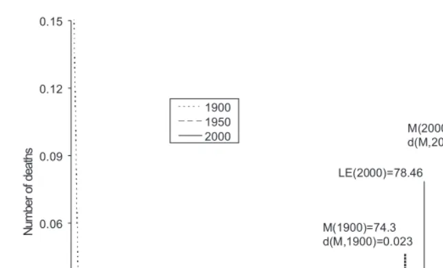
Figure 1: Life expectancy, LE, modal age after age 5,M, and modal num-ber of deaths,d(M), in the life table distribution of deaths for the Netherlands total population in 1900, 1950 and 2000
0.00 0.03 0.06 0.09 0.12 0.15
0 10 20 30 40 50 60 70 80 90 100 110+
Age
N
u
m
b
e
r
o
f
d
e
a
th
s
1900 1950
2000 M(2000)=84.58d(M,2000)=0.042
LE(1900)=48.39
LE(2000)=78.46
M(1900)=74.3 d(M,1900)=0.023
Source:Author’s calculations ofMandd(M)as explained in the appendix based on the Human Mortality Database (2008).
80. Assuming continuity over age in the life table functions, the modal age at death after
age 5 can be calculated as the age at which the derivative with respect to age ofd(a, t)is
equal to zero. From the relation in equation (1) and the productd(a, t) =µ(a, t)l(a, t),
the partial derivative of the distribution of deaths with respect to age is
∂d(a, t)
∂a =d(a, t)
·
∂ln [µ(a, t)]
∂a −µ(a, t)
¸
. (2)
Equation (2) is equal to zero whend(a, t)orh∂ln[∂aµ(a,t)]−µ(a, t)iare equal to zero.
In the first case there are no deaths, and therefore also no modal age. The second case
implies that at the modal ageM the force of mortality equals its relative derivative with
respect to age,
∂ln [µ(a, t)]
∂a =µ(a, t). (3)
This relation at the modal age proved to be interesting under the Gompertz model of mortality (Pollard 1991, Pollard and Valkovics 1992). To further add to this special age in the distribution of deaths, Wilmoth and Horiuchi (1999) showed that the modal age is also the inflection point in the survival curve.
Model populations provide a useful way to examine changes in mortality. In the next section the trend over time in modal age at death, the number of deaths and survivors at this age under four types of mortality models are assessed. The selected models change over age and time, and have been adopted by demographers as good approximations for the force of mortality (Thatcher et al. 1998).
3. Mortality models
3.1 Gompertz mortality change model
Bongaarts and Feeney (2002, 2003) have stimulated a new debate about how to interpret period summary measures of mortality when rates of death vary over time. The paral-lel shift in adult mortality analyzed by Bongaarts and Feeney can be characterized by a Gompertz mortality change model (Vaupel 1986, Vaupel and Canudas-Romo 2003). Their formulation is an extension of the Gompertz (1825) model of mortality, which has a changing force of mortality component,
µ(a, t) =µ(0, t)eβa, (4)
whereµ(0, t)reflects the value of the rate of mortality decrease over time and parameter
β >0is the fixed rate of mortality increase over age.
Substituting the Gompertz mortality change model in equation (3) and solving fora
gives us the modal age at timet, by lettingM =a,
M(t) =ln[β]−ln[µ(0, t)]
β . (5)
The survival function for this model is obtained by substituting the force of mortality of equation (4) in equation (1). At the modal age, (5), the survival function can then be simplified to
l(M, t) =e[µ(0β,t)−1], (6)
with a maximum number of deaths of
d(M, t) =l(M, t)µ(M, t) =βe[µ(0β,t)−1]. (7)
Bongaarts and Feeney (2002, 2003) showed that the value ofµ(0, t) declines over
time. When the reduction in mortality is almost negligible, and the value ofµ(0, t)
ap-proaches zero, equations (6) and (7) decrease to a constant number of survivors
lim
µ(0,t)→0l(M, t) =e
−1≈0.37, (8)
and thus the number of deaths isd(M, t) =βe−1(Pollard 1991, Pollard and Valkovics
1992). However, the modal age at death increases to infinity. Therefore, under this model the rectangularization process of the survival curve has stopped completely and no more
concentration is observed inl(M, t). Instead, a shift occurs in the modal age towards
A particular case of equation (4) is where theµ(0, t)is parameterized, and the force
of mortality at age 0 and timetisµ(0, t) = eα−ρt (Vaupel 1986, Schoen et al. 2004).
The force of mortality at ageaand timetis defined as
µ(a, t) =eα−ρt+βa, (9)
whereαis a constant that reflects the value of the force of mortality at age zero and time
zero,µ(0,0), and parameterρis the rate of mortality decrease over time.
In this model of continuous mortality decline, we set β = 0.11as the conventional
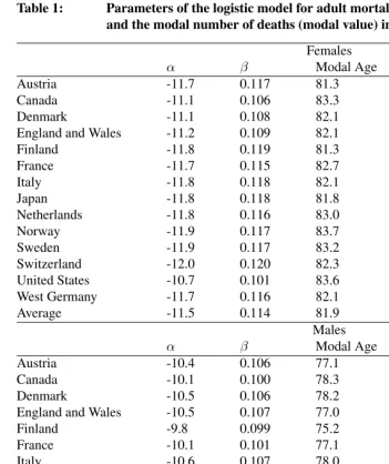
value for the pace of mortality increase over age (see the average row in Table 1).
Rea-sonable values for contemporary Western low mortality populations areα=−10.5and
ρ = 0.01(Bongaarts 2005, Schoen et al. 2004). Using these values and equations (5)
and (9), we obtain a modal age for timetofM(t) = 75.4 +³ρ
β ´
t, i.e., increasing one
year of age every eleven calendar years,βρ = 0.909. However, the survivors and number
of deaths in (6) and (7) change very modestly over time, reaching their limit values of
l(M) =e−1andd(M) =βe−1= 0.04, respectively.
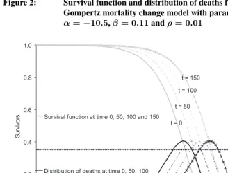
Figure 2 shows the survival function and distribution of deaths in the continuous de-clining mortality model (9) over 150 years.
As observed in Figure 2, the modal age increases every 50 years by 4.5 years of age. However, the number of survivors and deaths at the modal age remain constant (values underlying Figure 2 are shown in Table 2).
The shifting mortality model observed by Bongaarts and Feeney (2002) shows many implications for the survival function and the distribution of deaths. These authors have advanced some possible implications for this type of shift in mortality, e.g. the need to find alternative summary measures of mortality that take this shift into account. As shown here, for populations where mortality is concentrated at adult ages the modal age at death is a good candidate to asses the question: how long do we live? This model is not unique, however. These results are tested in the next subsections under alternative mortality models.
Figure 2: Survival function and distribution of deaths from a life table of a Gompertz mortality change model with parameters:
α=−10.5,β= 0.11andρ= 0.01
0.0 0.2 0.4 0.6 0.8 1.0
0 10 20 30 40 50 60 70 80 90 100 110 120
Age
S
u
rv
iv
o
rs
0.00 0.02 0.04 0.06 0.08 0.10
D
e
a
th
s
Survival function at time 0, 50, 100 and 150
Distribution of deaths at time 0, 50, 100 and 150
t = 0 t = 50
t = 100 t = 150
3.2 Logistic model
The logistic model has been used in place of the Gompertz model to account for the overestimation of mortality at older ages (Thatcher et al. 1998, Thatcher 1999). Bon-gaarts (2005) studied separately the two components of the logistic model, senescent and background mortality. Here only the senescent component is examined, because the back-ground component does not vary over age. The force of mortality is here expressed as
µ(a, t) = e
α(t)+β(t)a
1 +eα(t)+β(t)a, (10)
where the parametersα(t)for the level of mortality andβ(t)for the rate of increase in
can be found by applying the relation in equation (3) as
M(t) =ln [β(t)]−α(t)
β(t) . (11)
and the number of deaths at this modal age is
d(M, t) =l(M, t)µ(M, t) =
·
1 +eα(t) 1 +β(t)
¸ 1
β(t) β(t)
1 +β(t). (12)
Bongaarts (2005) examined change over time foreα(t)andβ(t)parameters in several
countries in the second half of the twentieth century. As noted by Bongaarts, the first
parameter decreased to levels around α(t) = −10.5, whileβ(t)has remained almost
constant around values of 0.11. According to these values, the number of deaths at the modal age is 0.038, just slightly less than the results for the Gompertz mortality change model.
If further decline in mortality is observed the parameter eα(t) will also continue to
decrease. In this case equation (12) depends only on the measure of the rate of increase in mortality with age. The survivors and distribution of deaths follow similar shifting patterns over time to those observed in Figure 2, because modal age at death continues
to increase with the change inα(t). As shown by Thatcher et al. (1998) and Thatcher
(1999), most mortality models fall between the overestimation of the Gompertz model and the logistic curve. Therefore, the constant value of deaths at the modal age is likely to appear in those models as well.
Table 1: Parameters of the logistic model for adult mortality, the modal age and the modal number of deaths (modal value) in 14 countries
Females
α β Modal Age Modal Value
Austria -11.7 0.117 81.3 0.0407
Canada -11.1 0.106 83.3 0.0371
Denmark -11.1 0.108 82.1 0.0377
England and Wales -11.2 0.109 82.1 0.0380
Finland -11.8 0.119 81.3 0.0413
France -11.7 0.115 82.7 0.0400
Italy -11.8 0.118 82.1 0.0410
Japan -11.8 0.118 81.8 0.0410
Netherlands -11.8 0.116 83.0 0.0404
Norway -11.9 0.117 83.7 0.0407
Sweden -11.9 0.117 83.2 0.0407
Switzerland -12.0 0.120 82.3 0.0417
United States -10.7 0.101 83.6 0.0354
West Germany -11.7 0.116 82.1 0.0404
Average -11.5 0.114 81.9 0.0397
Males
α β Modal Age Modal Value
Austria -10.4 0.106 77.1 0.0371
Canada -10.1 0.100 78.3 0.0351
Denmark -10.5 0.106 78.2 0.0371
England and Wales -10.5 0.107 77.0 0.0374
Finland -9.8 0.099 75.2 0.0347
France -10.1 0.101 77.1 0.0354
Italy -10.6 0.107 78.0 0.0374
Japan -10.7 0.108 78.6 0.0377
Netherlands -10.8 0.109 79.0 0.0381
Norway -10.8 0.109 79.1 0.0381
Sweden -11.1 0.112 79.7 0.0390
Switzerland -10.9 0.111 78.6 0.0387
United States -9.7 0.094 77.6 0.0331
West Germany -10.4 0.105 78.0 0.0367
Average -10.4 0.105 77.3 0.0367
Source:The logistic parameters come from the average of annual estimates for all available years from 1950 to 2000 from Bongaarts (2005).
3.3 Siler mortality change model
3.3.1 Siler model
The mortality models presented above assume that infant mortality has already declined and the distribution of deaths is only composed of deaths at senescent ages. However, the first stages of the epidemiological transition were characterized by a decline in infant mortality, which was followed later by declines at advanced ages (Omran 1971). There-fore, to have a complete understanding of the change over time in modal age at death and the modal number of deaths, it is necessary to include infant mortality and the premature component of the distribution of deaths.
The Gompertz model with a continuous rate of decline of equation (9), can be ex-tended to include these two additional components. A proposal by Canudas-Romo and Schoen (2005) combines the mortality model used by Siler (1979) and parameters that account for improvement in mortality over time
µ(a, t) =eα1−ρ1t−β1a+eα2−ρ2t+eα3−ρ2t+β3a, (13)
where three constant terms reflect the value ofµ(0,0) =eα1+eα2+eα3; the parameters
β1 andβ3 are fixed rates of mortality decline and increase over age, respectively, and
account for infant and senescent mortality; the parametersρ1andρ2are constant rates of
mortality decrease over time. Parametersαs andβs come from the Siler model, while the
ρs are used in Gompertz models with a continuous rate of decline (Vaupel 1986, Schoen
et al. 2004). In the remaining text I refer to equation (13) as the Siler mortality change model.
In the model we begin with a fairly high infant mortality (103 per thousand), resulting
from the values ofeα1 = 0.1,eα2 = 0.003 and eα3 = 0.00002. The early decline
over age proceeds at a pace ofβ1 = 1with an overall increase with age at a rate of
β3 = 0.11. At time 0, the modal age at death at advanced ages is 75.5, and the modal
number of deaths at this age is 0.028 deaths. These values approach those observed in populations with historical data. For example, in Sweden in the year 1900 the late modal age at death was 76.9 and the number of deaths at this age 0.024. For the pace of mortality
improvement we have chosenρ1 = 0.015andρ2 = 0.01. These values correspond to a
1.5% decline at younger ages and mortality improvement of one percent per year at older
ages. More details on the values for parametersα,β andρare discussed in
Canudas-Romo and Schoen (2005).
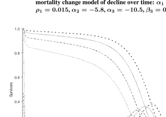
in infancy have very little probability of occurring during the ages of the premature deaths before the modal age. Therefore, the new survivors add to the distribution of deaths of senescent mortality and increase the modal number of deaths (values underlying Figures 3a and 3b are shown in Table 2).
Figure 3a: Survival function and distribution of deaths from a life table of a Siler mortality change model of decline over time:α1=−2.3,β1= 1,
ρ1= 0.015,α2= −5.8,α3=−10.5,β3 = 0.11andρ3= 0.01
0.0 0.2 0.4 0.6 0.8 1.0
0 10 20 30 40 50 60 70 80 90 100 110 120 Age
S
ur
vi
vo
rs
0.00 0.02 0.04 0.06 0.08 0.10
D
ea
th
s
0 50 100 150
3.3.2 Log-Siler model
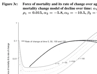
under the log-Siler model, it is interesting to look at the central relation that occurs at the modal age. At this age the force of mortality and the rate of change with respect to age are exactly the same, mathematically this is expressed in equation (3). Figure 3c shows this crossover point for the log-Siler model at time 0, 50, 100 and 150.
Figure 3b: Change over time in the modal age and modal number of deaths (modal value) under a Siler mortality change model of decline over time:α1 =−2.3,β1 = 1,ρ1= 0.015,α2 =−5.8,α3=−10.5,
β3= 0.11andρ3= 0.01
70 85 100 115 130
0 50 100 150 200 250 300 350 400 450 500
Year
M
od
al
A
ge
0.015 0.025 0.035 0.045
M
o
da
lV
a
lu
e
Modal Value
1. The modal age at death is strongly dependent on the force of mortality and its rate of change over age prevailing at older ages.
2. Changes in infant mortality are indirectly related to the modal age at death, by having an effect in the modal number of deaths.
Figure 3c: Force of mortality and its rate of change over age under a log-Siler mortality change model of decline over time:α1=−2.3,β1= 1,
ρ1= 0.015,α2= −5.8,α3=−10.5,β3 = 0.11andρ3= 0.01
0.0001 0.001 0.01 0.1 1
0 10 20 30 40 50 60 70 80 90 100 110 Age
F
or
ce
of
m
o
rt
al
ity
&
its
ra
te
of
ch
an
ge
0.0001 0.001 0.01 0.1 1
Rate of change at time 0, 50, 100 and 150
Death rate at time 0, 50, 100 and 150
t = 0 t = 50 t =100
t = 150
above models, the concentration of deaths around the modal age is analyzed in the next section.
4. Concentration of the number of deaths around the modal age at
death
Standard deviations around the late modal age at death have been used to study the dis-persion of deaths centred at the modal age at death (Kannisto 2001, Cheung et al. 2005, Cheung and Robine 2007). To prove the constancy of the concentration of deaths around
the mode, the standard deviation from the modal age at death, SDM, is studied. It is
defined as
SDM(t) =
v u u u t
ω Z
0
[a−M(t)]2d(a, t)da, (14)
whereωis the highest age attained in the population and the denominator of this measure
is equal to one, i.e. R0ωd(a, t)da= 1. SDM is parallel to the standard deviation around
the mean, and both measures are expressed in units of years of age (Wilmoth and Horiuchi
1999), although the centre of the observations is changed.SDM helps at quantifying the
bulk of deaths around the mode. This is different than the root mean square deviations
from M, which are positive, and used by Kannisto (2001), Cheung et al. (2005) and
Cheung and Robine (2007). The latter measure is a hypothetical number of deaths around the mode by considering only the experience of deaths above the mode and reflecting
it with respect to the mode. Opposed to this, SDM includes all the deaths below and
above the mode. The limitation of this measure is that it does not differentiate from child, premature and senescent mortality. However, for our purposes of measuring the constancy of the concentration of deaths around the mode it is the most appealing measure.
Table 2 presents the modal age, modal number of deaths, and the standard deviation from the mode for the Gompertz mortality change model of Figure 2 and equation (9), and the Siler mortality change model of Figures 3a and 3b, and equation (13).
As observed in Table 2 under both models the modal age at death increases linearly.
The modal number of deaths andSDM are nearly constants at values of 0.040 and 13,
Table 2: Modal age, modal number of deaths (modal value), and standard deviation from the mode,SDM, over 600 years (units of time) for a Gompertz mortality change model with parametersα = −10.5,
β = 0.11andρ = 0.01and a Siler mortality change model with parametersα1 = −2.3,β1 = 1,ρ1 = 0.015,α2 = −5.8,
α3=−10.5,β3 = 0.11andρ3= 0.01
Gompertz Mortality Change Model Siler Mortality Change Model
Modal Modal Standard Modal Modal Standard
Year Age Value Deviation Age Value Deviation
0 75.9 0.040 12.9 75.4 0.028 35.8 50 80.4 0.040 12.9 80.1 0.033 29.5 100 85.0 0.040 13.0 84.8 0.036 24.7 150 89.5 0.040 13.0 89.4 0.038 21.1 200 94.1 0.040 13.0 94.0 0.039 18.5 400 112.2 0.040 13.0 112.2 0.040 14.1 600 130.4 0.040 13.0 130.4 0.040 13.2
Under the mortality models analysed here we confirm that the rectangularization pro-cess of mortality compression dramatically decreases once infant mortality has become a minor factor. However, our results further the rectangularization debate by suggesting that the current situation might be the beginning of a shifting trend in mortality (Wilmoth and Horiuchi 1999, Kannisto 2000).
To this point we have analyzed the distribution of deaths and modal age at death under mortality model assumptions. In the next section we contrast the results presented above with those for changes in human populations with available time series of mortality.
5. Six industrialized countries: An illustration
time patterns caused by wars. The years of the influenza pandemic of 1918-1919 were taken out of the analysis because our interest is on overall time trends and not the year to year fluctuations.
Figure 4a, 4b and 4c show the change over time in the modal age at death, the modal
number of deaths and the standard deviation respect to the mode (SDM) in England and
Wales, France, Japan, Italy, Sweden, and the United States. The modal age at death and the modal number of deaths were calculated by fitting a quadratic curve as explained in the appendix.
Figure 4a shows an increasing linear trend in the modal age at death for the six coun-tries examined, although at different increasing pace from country to country. At the beginning of the Japanese series low values for modal age at death are observed, but this country rapidly changed to become the country with the highest value, followed closely by France. The modal age in England and Wales changed at a modest pace, continuing to exhibit the lowest values for this group of countries in the most recent years together with the US. Figure 4b displays the logistic trend in the number of deaths at the modal age for the six selected countries. The trend over time is less clear than for the modal age at death. However, we find an increase from low to high values and levelling off in the second half of the century. The last decade of the century reveals unexpected changes, which include a decline for Japan and an increase for the other countries. These changes have not been followed by any sudden expansion in the distribution of deaths in Japan and concentration in this distribution for the other countries (Figure 4c). As seen in Figure 4c, the common
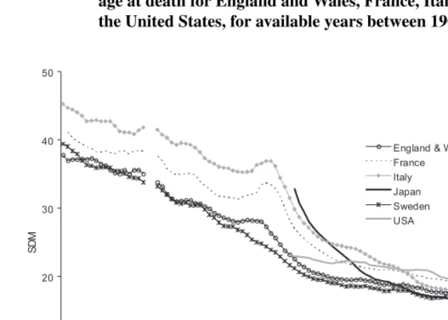
trend for all the countries is a decline inSDM over time, although at different levels from
country to country. In the most recent years, Sweden has the strongest compression, as
measured by theSDM, and the values ofSDM in the United States are much higher than
for the other countries.
6. Discussion
Figure 4a: Five year moving average of the modal age at death for England and Wales, France, Italy, Japan, Sweden and the United States,
for available years between 1900 and 2005
65 70 75 80 85 90
1900 1910 1920 1930 1940 1950 1960 1970 1980 1990 2000 Year
M
od
al
a
ge
65 70 75 80 85 90
England & Wales France Italy Japan USA Sweden
Source: Authors’ calculations based on Human Mortality Database (2008). The years of the influenza epidemic 1918-1919 have been excluded.
The empirical results of the modal age at death, and theSDM in Figures 4a and 4c
populations at each age there is great variation in the rate of improvement of mortality over time (Vaupel and Canudas-Romo 2003).
Figure 4b: Five year moving average of the modal number of deaths for England and Wales, France, Italy, Japan, Sweden and the United States, for available years between 1900 and 2005
0.015 0.025 0.035 0.045
1900 1910 1920 1930 1940 1950 1960 1970 1980 1990 2000 Year
M
od
al
va
lu
e
0.015 0.025 0.035 0.045
England & Wales France Italy Japan Sweden USA
Source: Authors’ calculations based on Human Mortality Database (2008). The years of the influenza epidemic 1918-1919 have been excluded.
7. Conclusion
where the compression of mortality has stopped, may be a realistic description of the current situation in low mortality countries.
Figure 4c: Five year moving average of the standard deviation from the modal age at death for England and Wales, France, Italy, Japan, Sweden and the United States, for available years between 1900 and 2005
0 10 20 30 40 50
1900 1910 1920 1930 1940 1950 1960 1970 1980 1990 2000 Year
S
D
M
0 10 20 30 40 50
England & Wales France Italy Japan Sweden USA
Source: Authors’ calculations based on Human Mortality Database (2008). The years of the influenza epidemic 1918-1919 have been excluded.
Mortality models, adopted as good approximations for the force of mortality, show that the modal age at death increases over time. However, the number of survivors and deaths at the modal age move towards constant levels. The distribution of deaths around the modal age and standard deviation from the mode also show a constant concentration -almost a reallocation- of the characteristic distribution around the modal age at death towards more advanced ages.
transition period to a shifting mortality scenario. The interest of the present research is to show overall patterns of mortality over time, but it cannot be discarded the possibility of reversals or accelerations in mortality during the transitional period. Future studies of the shape of distribution of deaths by cause of death could improve our understanding of the dynamics of mortality and their distribution.
Finally, the rectangularization of the survival curve is characterized by a change from a wide dispersion of deaths to a concentration in the number of deaths. Although it de-scribes the mortality changes observed in the last half of the century well, it might only be a temporary phenomenon. The shifting mortality scenario studied in this article might also be transitory, yet it brings light to alternative processes that might be expected if the current mortality changes maintain their pace.
8. Acknowledgements
References
Barbi, E., Bongaarts, J., and Vaupel, J. W. (2008).How Long Do We Live?: Demographic
Models and Reflections on Tempo Effects.Berlin: Springer.
Bongaarts, J. (2005). Long-range trends in adult mortality: Models and projection meth-ods.Demography, 42(1):23–49.
Bongaarts, J. and Feeney, G. (2002). How long do we live? Population and Development
Review, 28(1):13–29.
Bongaarts, J. and Feeney, G. (2003). Estimating mean lifetime. Proceedings of the
Na-tional Academy of Sciences, 100(23):13127–13133.
Canudas-Romo, V. (2006). The modal age at death and the shifting mortality hypothe-sis. Presentation at the Population Association of America 2006 meeting held in Los Angeles, California.
Canudas-Romo, V. and Schoen, R. (2005). Age-specific contributions to changes in the
period and cohort life expectancy.Demographic Research, 13(3):63–82.
Canudas-Romo, V. and Wilmoth, J. R. (2007). Record measures of longevity. Presentation at the Population Association of America 2007 meeting held in New York.
Cheung, S. L. K. and Robine., J. M. (2007). Increase in common longevity and the
compression of mortality: The case of Japan.Population Studies, 61(1):85–97.
Cheung, S. L. K., Robine, J. M., Jow-Ching Tu, E., and Caselli, G. (2005). Three dimen-sions of the survival curve: Horizontalization, verticalization, and longevity extension. Demography, 42(2):243–258.
Feeney, G. (2006). Increments to life and mortality tempo. Demographic Research,
14(2):27–46.
Fries, J. (1980). Aging, natural death, and the compression of morbidity. New England
Journal of Medicine, 303(3):130–35.
Goldstein, J. R. (2006). Found in translation?: A cohort perspective on tempo-adjusted
life expectancy.Demographic Research, 14(5):71–84.
Gompertz, B. (1825). On the nature of the function expressive of the law of human
mor-tality and on a new mode of determining life contingencies.Philosophical Transactions
of the Royal Society of London, 115:513–85.
Guillot, M. (2006). Tempo effects in mortality: An appraisal. Demographic Research,
14(1):1–26.
13(8):189–200.
Horiuchi, S. and Wilmoth, J. R. (1998). Deceleration in the age pattern of mortality at
older ages.Demography, 35(4):391–412.
Human Mortality Database. University of California, Berkeley (USA), and Max Planck Institute for Demographic Research (Germany). Available at www.mortality.org or www.humanmortality.de (data downloaded on [01/29/2008]).
Janssen, F. and Kunst., A. (2007). The choice among past trends as a basis for the
predic-tion of future trends in old-age mortality. Population Studies, 61(3):315–326.
Kannisto, V. (2000). Measuring the compression of mortality. Demographic Research,
3(6).
Kannisto, V. (2001). Mode and dispersion of the length of life. Population: An English
Selection, 13:159–71.
Lee, R. D. and Carter, L. R. (1992). Modeling and forecasting US mortality. Journal of
the American Statistical Association, 87(419):659–671.
Lexis, W. (1878). Sur la duree normale de la vie humaine et sur la theorie de la stabilite des rapports statistiques. [on the normal human lifespan and on the theory of the stability
of the statistical ratios]. Annales de Demographie Internationale, 2:447–60.
Nusselder, W. J. and Mackenbach, J. P. (1996). Rectangularization of the survival curve
in the Netherlands, 1950-1992.The Gerontologist, 36(6):773–783.
Omran, A. (1971). The epidemilogical transition. Milbank Memorial Fund Quarteyly,
49:509–38.
Pollard, J. H. (1991). Fun with Gompertz.Genus, 47(1-2):1–20.
Pollard, J. H. and Valkovics, E. J. (1992). The Gompertz distribution and its applications. Genus, 48(3-4):15–28.
Robine, J. M. (2001). Redefining the stages of the epidemiological transition by a study
of the dispersion of life spans: The case of France. Population: An English Selection,
13:173–93.
Rodriguez, G. (2006). Demographic translation and tempo effects: An accelerated failure
time perspective.Demographic Research, 14(6):85–110.
Schoen, R. and Canudas-Romo, V. (2005). Changing mortality and average cohort life
expectancy.Demographic Research, 13(5):117–142.
University, University Park PA.
Siler, W. (1979). A competing-risk model for animal mortality.Ecology, 60(4):750–57.
Thatcher, A. R. (1999). The long-term pattern of adult mortality and the highest attained age.Journal of the Royal Statistical Society, 162 Part 1:5–43.
Thatcher, A. R., Kannisto, V., and Vaupel, J. W. (1998).The Force of Mortality at Ages 80
and 120. Odense Monographs on Population Aging 5. Denmark: Odense University Press.
Vaupel, J. W. (1986). How change in age-specific mortality affects life expectancy.
Pop-ulation Studies, 40:147–57.
Vaupel, J. W. (2005). Lifesaving, lifetimes and lifetables. Demographic Research,
13(24):597–614.
Vaupel, J. W. and Canudas-Romo, V. (2003). Decomposing change in life expectancy:
A bouquet of formulas in honor of Nathan Keyfitz’s 90th birthday. Demography,
40(2):201–16.
Wachter, K. W. (2005). Tempo and its tribulations. Demographic Research, 13(9):201–
222.
Wilmoth, J. and Horiuchi, S. (1999). Rectangularization revisited: Variability of age at
death within human populations.Demography, 36(4):475–95.
Wilmoth, J. R. (1997). In search of limits. In Wachter, K. W. and Finch, C. E., editors, Between Zeus and the Salmon. The Biodemography of Longevity. National Academy Press: Washington (DC).
Wilmoth, J. R. (2005). On the relationship between period and cohort mortality.
Appendix
This appendix includes some specific calculations used in this study.
1. For countries with available data, the modal age at death was calculated by using Kannisto’s (2001) proposal of modal age with decimal precision. To calculate the modal number of deaths Kannisto’s quadratic function assumption has been
ap-plied. Letxbe the age with the highest number of deaths in the life table at timet,
d(x, t). The number of deaths at agesx,x−1andx+ 1are used to fit a quadratic
polynomial to the function describing the death distribution,d(a, t). The quadratic
function has parametersα(t),β(t)andγ(t)that change over time,
d(a, t) =α(t)a2+β(t)a+γ(t). (A1)
The modal age at death with decimal point precision is found at the ageM(t) =
−2βα((tt)). In terms of the ages and distribution of deathsd(a, t)the expression of the
modal age at death is
M(t) =x−0.5 + [d(x, t)−d(x−1, t)]
[d(x, t)−d(x−1, t)] + [d(x, t)−d(x+ 1, t)], (A2)
wherexis the age with the highest number of deaths in the life table at timet,
d(x, t). This calculation is correct for a life table that changes continuously over
age in which cased(x, t)represents the exact number of deaths at agex,d(x, t) =
µ(x, t)l(x, t). For life tables of one year age-groups the function describing the
distribution of deaths should be put at the middle of the interval at age x+ 0.5,
which changes equation (A2) to be exactly Kannisto’s proposal. The modal number of deaths is calculated by substituting the value of the mode in equation (A1) as
d(M(t), t) =−β(t) 2
4α(t) +γ(t). (A3)
2. Equation (3) includes the force of mortality and its relative derivative with respect to age. The force or mortality is calculated as the relative derivative of the life table survival function as
µ(a, t) =−∂ln[l(a, t)]
∂a . (A4)
When data were available for two agesaanda+kthe following approximation for
the relative derivative with respect to time of the functionl(a, t)was used:
∂ln[l(a, t)]
∂a ≈
lnhl(la(+a,tk,t))i
Similarly the partial derivative with respect to age for the functionµ(a, t)was cal-culated as
∂ln[µ(a, t)]
∂a ≈
ln
h µ(a+k,t)
µ(a,t)
i
k . (A6)