Online at http://desert.ut.ac.ir
Desert 23-2 (2018) 211-220
Comparison of spectrum indices for mapping soil salinity in
saline lands of Chezan plain (Markazi province)
A. Ahmadi
a*, A. Kazemi
b, H. Toranjzar
ca
Department of Rangeland Science, Islamic Azad University, Arak branch, Arak, Iran
b Department of Environment Sciences, Faculty of Agriculture and Natural Resources, Arak University, Arak, Iran c Islamic Azad University, Arak branch, Arak, Iran
Received: 31 May 2017; Received in revised form: 10 September 2018; Accepted: 16 September 2018
Abstract
Soil salinity phenomena are one of the main problems of arid and semi-arid lands. Saline soils constitute a huge part of Iran, and also threaten its neighboring lands. Therefore, in order to optimum exploitation of such soils, qualitative monitoring is necessary. Recently, remote sensing techniques have been increasingly applied in monitoring soil characteristics. The present study was carried out between 2014 and 2015, with the purpose of using remote sensing for mapping soil salinity in the saline rangelands of Chezan plain (Markazi province). In the first step, 50 soil samples were taken from the topsoil (30 cm depth) and their Electrical Conductivity (EC) was measured by EC- meter. To use the soil salinity map using remote sensing, we first used Indian Remote sensing Satellites (IRS) satellite imagery and the satellite’s LISS sensor (LISS III, 2008). After geometric and radiometric correction, this image was been classified using the Maximum Likelihood method. Then in the next step, Comparison of Spectrum indices were done by extracting maps of soil salinity. For this purpose, Four indices including: Brightness Index (BI), Salinity Index (SI1), SI2, and Normalized Difference Salinity Index (NDSI) were used. Among these indices, SI2 had the most correlation with ground control points (0.63 in 1% level) and is introduced as a more suitable index than others for zoning soil salinity. Regarding to the salinity map, the results showed that a sizeable portion of the study area was classified class 2 with a salinity of between 4-8 dS/m (55% of whole land).
Keywords: Soil salinity; LISS III; Spectrum Index; Remote sensing; Chezan
1. Introduction
In the present century, the population increase has resulted in destroying vegetation and changing landscapes, especially in arid and semiarid regions, which constitute as fragile ecosystems that cover 35% of the earth’s land surface (Ziadat et al., 2012). Saline lands are more susceptible to erosive factors: salinity and alkalinity are two major phenomena leading to soil degradation in arid and semi-arid areas. Soil salinity is an in-situ form of soil degradation due to the buildup of soluble salts at the surface soil (Bouaziz et al., 2012). Saline soils occupy about 23 million hectares (15%) of the total area of Iran and there are about 163 halophyte and
Corresponding author. Tel.: +98 86 33412190 Fax: +98 86 33412190
E-mail address: [email protected]
Salt tolerant species in Iran (Ahmadi et al., 2013). According to the United States Environmental Protection Agency, about 20% of the world’s fields suffer from salinity, and soil salinity is a huge limitation impeding the use of agricultural lands (Rezaie et al., 2006). The degradation of soil quality due to natural and anthropological factors is a major concern because it threatens the sustainability and food production of humans. In particular, there is general agreement that soil salinity is a major threat to irrigated and rain-fed agriculture throughout the world (Scudiero et al., 2015). Soil salinity inhibits cell water uptake in plants and also causes the aggregation of Na+
and Cl-, and getting nutrition by the mutual
essential for optimum exploitation of such soils, especially in agricultural activities.
Salinity assessment and mapping are traditionally conducted by soil surveys and the interpolation of analytical results of soil samples. However, such conventional means of soil survey requires the investment of a great deal of time and funding (Wu et al., 2014). Current developments in the use of remote-sensing technology in the mapping and managing of saline lands have led to increases in the speed and accuracy and decreases in related fees (Taher Kia, 1999). Remote sensing is superior to conventional methods for drought and salinity monitoring (Safari Shad et al., 2017), as this technology can predict soil salinity and provide impact assessment. It saves labor, time and effort when compared to conventional field measurements. The information derived from remote sensing tools is significantly objective, and covers a wide region, and the data provided gives us information on salt-affected soils of both spatial and temporal natures.(Abbas et al., 2013). Many studies have been conducted through satellite imagery to investigate salinity. Nawar et al. (2014)studied the potential of remote sensing in estimating and mapping soil salinity in the El-Tina Plain, Egypt. They constructed two predictive models based on the measured soil’s electrical conductivity (ECe) and laboratory soil reflectance spectra were resampled to the Landsat sensor’s resolution in keeping with the PLSR model. The results indicated that MARS is a more suitable technique than PLSR for the estimation and mapping of soil salinity, especially in areas with high levels of salinity. Dashtakian et al. (2009) used several methods to produce the soil salinity map of Marvast, (Yazd) including Brightness Index (BI), Normalized Difference Salinity Index (NDSI), Salinity Index (SI), Yazd Salinity Index (YSI), and the maximum likelihood and average of regression with some Bands. By analyzing and comparing methods with the actual soil salinity map, the most suitable methods for this region were found to be: 1. Average regression with standardized band 1,2 and 3. 2. Salinity index method.
Azhirabi et al. (2015) used different vegetation-based indices such as SI1, SI2, SI3, BI, NDSI, PD322, IPVI and DVI, which were extracted from ETM+ (Landsat 7) to map soil salinity in the army field of Gorgan. Also, the brightness value was determined. Their results showed that among SIs, SI1 and SI2 had the highest capability to provide salinity maps with the most correlation with land data.
Dehni and Lounis (2012) applied the remote sensing technique in mapping salt affected soils in the Oran region of Algeria. Their approach was to exploit the multi-spectral optical data from the LANDSAT ETM + to map surface states using indices of salinity and sodicity as: BI, NDSI, SI, ASI, Index of Salinity (using GIS and remote sensing), and finally SSSI “Soil Salinity and Sodicity Index”. These indicators of salinity were tested in the Oran region using spectral sensor ALI (Advanced Land Imager) from satellite EO-1 (NASA from 2002 to 2006).
Hakimzadeh and Vahdati (2018) monitored Electrical Conductivity (EC) for the soil salinity index and Organic Matter (OM) using IRS (LISS III) satellite images in the area of Harat (Yazd). Results showed that during the period stretching between 2008-2012 the organic matter content of all farmlands increased and the area of saline land decreased.
Since most of the rangelands in Markazi province and Chezan plain have faced the danger of salinization and alkalization, this study was carried out with the purpose of capturing images using the IRS satellite’s LISS III sensor, and comparing spectrum-indices to prepare the soil salinity map.
2. Materials and Methods
2.1. Study area
The study area is located in the Chezan plain at the following coordinates: 49 ˚ 8' 22"E to 49˚ 10' 9"E and 33 ˚ 32' 5"N to 34 ˚ 33' 37"N (Fig. 1). This area has saline and alkaline soils dominated by Comphorosma monspeliaca, a halophyte range plant (Fig.2). The average annual precipitation is about 255 mm and mean height is 1644 m a.s.l. The annual mean temperature of the study area is 14.2 C˚. According to soil taxonomy (2014), the gypsic and salic diagnostic horizons were separated and the study area’s soil was classified in the aridic order.
2.2. Soil sampling
Fig. 2. Geographic location of study area and sampling points
Fig. 3. Vegetation type of Chezan saline rangelands including Comphorosma monspeliaca shrubs
2.3. Geometric correction and images classification
Definite and suitable parts of the land with a clear geographical location should be selected for geometric correction. These locations should
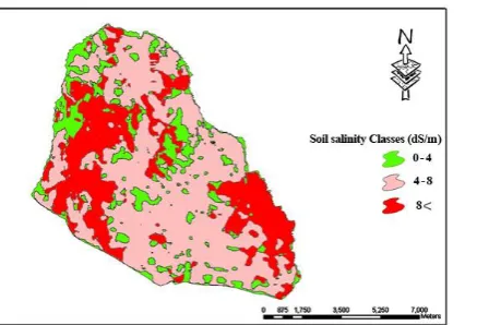
The classification of satellite images was done in 3 classes of soil salinity including: class 1: low salinity, class 2: medium salinity, and class 3: high salinity. In the next step, class classification was calculated based on the Jefferies Matusita index and the maximum likelihood method, the results of which have been shown as maps (Fig.4 to Fig.8). The areas of each soil salinity class were calculated in ArcGIS ver. 10. Software (Table5).
The Jeffries–Matusita (JM) distance is widely used as a separability criterion for optimal band selection and evaluation of classification results (Table 5). The Jeffries-Matusita distance measures the separability of two classes on a more convenient scale [2-0] in terms of B: J=2(1-e^⁻B)
Normality test for spectrum indices
Regarding the different ability of each index in presenting a soil salinity map, first, data
normality was tested using SPSS. As the significance for all indices and all collected soil data was more than 5%, null hypothesis will not rejected and data will be normal (Chahoki, 2010).
3. Results and Discussion
3.1. Determination of best band combination and evaluation of the land use map accuracy
In selecting the best band combination, Table 1 was used. In this Table, Cohen's kappa coefficient and the total correction for different band combination of sensor LISSIII were observed. The results revealed that this sensor, with a band combination of band 1, MNF (Minimum Noise Fraction) 1, and PC1 which are settled in RGB, will show the highest accuracy, and thus were introduced as the best band combination.
Table 1. Cohen's kappa coefficient and total accuracy of the band combination of different bands of LISSIII Image type Band combination Cohen's kappa coefficient Total accuracy
LISSIII Band 4,3,2 0.61 64.15%
Band 2,3,PC2 0.74 78.10%
Band1, MNF1, PC1 0.79 86.60%
Band3, PC1, MNF1 0.63 69.21%
Band 4, SAVI, 3 0.61 72.78%
Band 3, PC1, 1 0.66 73.31%
Band 2, PC1, NDVI 0.65 70.98%
After assurance of correct classification, each soil salinity class area were calculated with Arc GIS.
3.2. Image classification
Mapping soil salinity with spectrum indices
With remote sensing, the soil salinity index can be derived from image using mathematical process on main sensor’s bands and many maps with spectrum characters could be extracted. The most important indices for soil salinity are: brightness index (BI), salinity index (SI), normalized different salinity index (NDSI), and others (Dehni and Lounis, 2012). Azhirabi et al. (2015) also used different vegetation-based indices such as SI1, SI2, BI, NDSI, etc., which were extracted from ETM+ (Landsat 7) to map soil salinity, and found, based on accuracy tests on studied indices that SIs had the most correlation with ground control points. In the present study, some spectral indices including: BI, NDSI, SI1, and SI21 were used and
1Salinity index 2
different maps for each index were prepared. Creation classes were based on image interpretation and experimental data. Four salinity classes were determined. After applying map classification, produced maps were subjected to final processing. For this purpose, a 5*5 filter was employed to decrease spatial diversity on maps.
Correlation test of spectrum indices
The correlation among maps extracted from the indices and real data (ground control points) of the study area were collected after insurance of data normalization. The extracted map of spectral indices showed high correlation with the real soil map. (Table 4).
So, for the evaluation of class accuracy other parameters such as user accuracy and producer accuracy must also be taking into consideration,
and the commission errors and omitted errors were also mentioned in Table 2.
Table 2. Evaluation of classification results for Chezan plain Index Salinity Class
(dS/m)
User accuracy Producer accuracy Commission errors
Omission errors
BI 0-4 77.50 64.75 8.5 4.35
4-8 94.57 91.46 6.76 7.80
More than 8 83.61 91.75 9.46 7.45
Having and omitted errors related to the classes of the soil salinity map for the SI2 index were investigated. The most and the least having errors were related to the 0-4 dS/m class
(8.50) and over 8 dS/m class (9.46). In addition, the most and the least omitted errors were related to the more than 8 class and 0-4 dS/m.
Table 3.Results of index normality test (Kolmogorov–Smirnov test) Kolmogorov–Smirnov test
SI1 SI2 NDSI BI EC1
Number 50 50 50 50 50
Normal Parametersa,,b Average 140.36 1.946 .1347 158.08 4.84 Standard deviation 14.821 5.266 .02648 12.673 1.638
Most Extreme Differences
Absolute 0.130 0.126 0.202 0.114 0.109
Positive 0.098 0.105 0.135 0.106 0.097 Negative -0.130 -0.126 -0.202 -0.114 -0.109 Kolmogorov-Smirnov Z 0.922 0.892 1.429 0.804 0.774
Asymp. Sig. (2-tailed) 0.364 0.404 0. 304 0.537 0.587
Table 4. reveals that SI2 has the most correlation with soil salinity. Therefore, the present map of this index was used as the soil
salinity map using remote sensing for the study area.
Table 4. Correlation among values of brightness and soil salinity data in different indices
BI SI1 NDSI SI2 EC
BI Pearson Correlation 1 Sig. (2-tailed)
N 50
SI1 Pearson Correlation 0.967** 1 Sig. (2-tailed) 0.000
N 50 50
NDSI Pearson Correlation 0.290* 0.417** 1 Sig. (2-tailed) .041 0.003
N 50 50 50
SI2 Pearson Correlation 0.989** 0.983** 0.358* 1 Sig. (2-tailed) 0.000 0.000 0.011
N 50 50 50 50
EC Pearson Correlation 2.6 0.52 -0.084 0.63** 1 Sig. (2-tailed) 0.661 0.722 0.560 0.663
N 50 50 50 50 50
** represents significance at the 0.01 level (2-tailed) * represents significance at the 0.05 level (2-tailed)
The result of the study revealed that the electrical conductivity of the Chezan plain ranges between 2.4 to 8 dS/m. After an
Fig. 4. Soil salinity classification map of the Chezan plain extracted from LISSIII image
Table 5. Separation of EC classes based on the Jefferies Matusita index (LISSIII image) Soil salinity class dS/m Jefferies Matusita index LISSIII
EC 0-4 1.91
EC 4-8 1.93
EC> 8 1.90
3.2. Classification accuracy
Having errors, show that each area of land is a class that does not truly belong to that class, and omitted errors show the amount of land area of a class that belongs to other classified classes. The most and the least omitted errors are related to the class 8 d S/m and above which equals11.71, and the 0-4 dS/m class equals 7.63 and the most and the least omitted errors are related to class 4-8 and class 0-4 dS/m, respectively (Table 6).
3.3. Soil salinity classes areas
Table 7 represents the area of each class and area percentage of the related class.
BI (brightness index) map
Figure 5 shows the map extracted from the BI index in which most of the area has a salinity that lies between 4-8 ds/m (class 2).
Table 6. Accuracy evaluation of classification results
Year Salinity class dS/m User accuracy Producer accuracy Having error Omitted error
2008 0-4 92.37 95.51 7.63 4.49
4-8 93.22 89.81 7.58 10.19
More than 8 88.29 82.83 11.71 7.17
Table 7. Areas of each soil salinity class in Chezan plain (2008)
Soil salinity class Areas (hectare) Area (%)
0-4 1349. 8239 15.29
4-8 7897. 4901 55.55
more than 8 7456. 2572 29.15
total 4671. 8824 100
NDSI (Normalized Difference Salinity Index) map
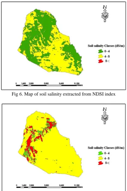
Figure 6 reveals the map derived from the NDSI index. Most areas of land are located in classes 1 and 2 (salinity of 0-4 and 4-8 dS/m.).
SI1 (salinity index 1) map
Figure 7, which was concluded from the study area’s salinity index reveals that most areas of land are class 2 (EC 4-8 dS/m).
Fig 6. Map of soil salinity extracted from NDSI index
Fig 7. Map of soil salinity extracted from SI1 index
SI2
Figure 6 represents the map extracted from salinity index 2 for the investigated location.
The most areas of land are class 2, meaning a salinity of 4-8 dS/m (Similar to SI1).
As mentioned before, SI2 has the most correlation in level 0.01 with soil salinity. Therefore, the present map of this index was used as map of soil salinity for the study area. In
table 8, the area of each class and its percentage (based on SI2 map) vis-à-vis the whole area is presented.
Table 8. Areas of different soil salinity classes based on SI2 index for Chezan plain
Soil salinity classes Area (hectare) Area percentage
0-4 438.084 4.96
4-8 7646.388 86.65
more than 8 739.886 8.38
total 8824.592 100
Several studies have shown that image enhancement techniques consisting of spectral indices (e.g., NDVI, SI, NDSI, TNDVI) have a great potential in enhancing and delineating soil salinity detail in an image. For example, Zhang et al. (2011) found and emphasized that identifying salt-affected soils based on the image enhancement method, represented by the salinity index, yields better results than individual bands, due to its ability to enhance the saline patches by suppressing the vegetation. Allbed et al. (2014) also reported that the high performance of combined models for mapping soil salinity is attributed to: (i) the spatial resolution of the images; (ii) the great potential of the enhanced images, derived from SI, by enhancing and delineating the spatial variation of soil salinity. Shamsi et al. (2013) found that using an image enhancement method (Salinity Index (SI)) reduced estimation errors and increased the model’s efficiency.
According to the extracted maps, the northern and western lands of study area are more saline. This may be due to land form and topsoil conditions. Because soil salinity spectral reflectance is affected by the physical-chemical properties of soil: quality and mineralogy of salt, together with soil moisture, color and surface roughness (Allbed et al., 2014) The result also indicates that the measured spectral reflectance and IRS data have great potential for predicting and mapping soil salinity. This finding is in agreement with Hakimzadeh and Vahdati (2018) who indicated that remote sensing data, especially IRS-LISIII, are highly efficient in the detection of soil salinity.
4. Conclusions
Soil salinity, either naturally occurring or human-induced, is a serious global environmental problem, especially in arid and semi-arid regions. This is a complex dynamic process with serious consequences for the soil , not to mention its geochemical, hydrological, climatic, agricultural, and economic impacts. Being a severe environmental hazard, the
frequent detection of soil salinity and assessment of its extent and severity at an early stage become very important at both local and regional scales. Traditionally, soil salinity was assessed via collecting in situ soil samples and analyzing those samples in the laboratory. Undertaking this method, especially over a large area, is expensive and time-consuming. Remote sensing represents a good alternative for monitoring and mapping changes in soil salinity.
Remote sensing data have been used extensively to identify and map saline areas, and the potential of remote sensing for assessing and mapping soil salinity is enormous. Multispectral satellite sensors are the preferred method for mapping and monitoring soil salinity, largely due to the low cost of such imagery and the ability to map extreme surface expressions of salinity.
important factors as well. The results of the study revealed that in the mapping of soil salinity, the use of remote sensing techniques are better because of their high accuracy and low cost. However, regarding the low separation and radiometric power of sensors, salinity changes are not tangible and traceable. Salinity is a parameter that indirectly reflects waves (contrary to vegetation cover) Thus, in order to achieve the best index we need high resolution and more vast extended areas to obtain the best results, so as to define the reliable local index.
This study offered a good method for the quantitative mapping of soil salinity over a large area with multispectral reflectance data. Further research could be done to reduce spectral noise in multispectral imaging and refine prediction models to improve the accuracy in the quantitative mapping of soil salinity.
Acknowledgment
Special thanks to the research and technology department of Islamic Azad University, Arak branch, for their financial and spiritual support, who made this study possible.
References
Abbas, A., S. Khan, N. Hussain, M. A. Hanjra, S. Akbar, 2013. Characterizing soil salinity in irrigated agriculture using a remote sensing approach. Physics and Chemistry of the Earth, 55-57; 43–52. Adel, M. A., Mahmoud, I. Mohd Hasmadi, M. S. Alias,
A. Mohamad Azani. 2016. Rangeland Degradation Assessment in the South Slope of the Jabal Al-Akhdar, Northeast Libya Using Remote Sensing Technology. Journal of Rangeland Science, 6; 73-81.
Ahmadi, A., M. Gomarian,M. Sanjari, 2013. Variations in Forage Quality of Two Halophyte Species,
Camphorosma monspeliaca and Limonium iranicum
at Three Phenological Stages. Journal of Rangeland Science, 3; 245-251.
Alkuwari, N.Y., M.F. Kaiser. 2011. Impact of North Gas Field development on land use/landcover changes at Al Khore, North Qatar, using remote sensing and GIS. Applied Geography, 31; 1144-1153.
Allbed, A., L. Kumar, P. Sinha, 2014. Mapping and Modelling Spatial Variation in Soil Salinity in the Al Hassa Oasis Based on Remote Sensing Indicators and Regression Techniques, Remote Sensing, 6; 1137-1157.
Azhirabi, R., B. Kamkar , A. Abdi, 2015. Comparison of different indices adopted from Landsat images to map soil salinity in the army field of Gorgan. J. of Soil Management and Sustainable Production, 5; 173-186.
Baboo, S., M.R. Devi. 2011. Geometric Correction in Recent High Resolution Satellite Imagery: A Case
Study in Coimbatore, Tamil Nadu. International Journal of Computer Applications, 14; 32-37. Bouaziz, M., J. Matschullat, R. Gloaguen, 2011.
Improved remote sensing detection of soil salinity from a semi-arid climate in Northeast Brazil. Comptes Rendus Geoscience, 343; 795-803. Bradley, A.P., 1997. The use of the area under the ROC
Curve in the evaluation of machine learning algorithms, Pattern Recognition, 30; 1145-1159. Bresler, E., R. J. Wagnet, A. Laurter, 1984. Statistical
analysis of salinity and texture effects on spatial variability of soil hydraulic conductivity. Soil Sci. Soc. Am. G, 78; 16-25.
Bruria, H., N. Arie, 1998. Physiological response of potato plants to soil salinity and water deficit, Plant science, 137; 43- 51.
Dashtekian, K., M. Pakparvar and J. Abdollahi,2009. Study of soil salinity preparing methods by using landsat images in Marvast. Iranian journal of Range and Desert Research, 15; 139-157.
Dehni, A., M. Lounis, 2012. Remote Sensing Techniques for Salt Affected Soil Mapping: Application to the Oran Region of Algeria. Procedia Engineering. 33; 188-198.
Metternicht, G.I., J.A. Zinck, 2003. Remote sensing of soil salinity: potentials and constraints. Remote Sensing of Environment, 85; 1-20.
Moustafa,M. M., A. Yomota, 1998. Spatial modeling of soil properties for subsurface drainage projects. Jour. Irrigation and Drainage Eng, 124; 218-228. Nawar, S., H. Buddenbaum, J. Hill, J. Kozak, 2014.
Modeling and Mapping of Soil Salinity with Reflectance Spectroscopy and Landsat Data Using Two Quantitative Methods (PLSR and MARS), Journal of Remote Sensing, 6; 10813-10834. Odeh, I. O. A., A. B. McBratney, D. J. Chittlebourough,
1995. Further results on pridictioin from terrain attributes: heterotopic cokriging and regression- kriging. Geoderma, 67; 512-236.
Peter, J., L.S.M. Vaughan, D.L. Corwin, D.G. Gone, 1995. Water content effect on soil salinity prediction, A geostatistecal study using co-kriging. Soil Sci. Soc. Am. Jour., 59; 1146-1156.
Rezaie, M. A., R. A. Khavari Nezhad and H. Fahimi. 2006. The effect of natural soil salinity on myeloperoxidase activates of two types of cotton. Fundamental science of IAU, 62; 79-89.
Safari Shad, M., A. Ildoromi, D. Akhzari, 2017. Drought Monitoring Using Vegetation Indices and MODIS Data (Case Study: Isfahan Province, Iran). Journal of Rangeland Science, 7; 148-159.
Scudiero, E., T. H. Skaggs, D. L. Corwin, 2015. Regional-scale soil salinity assessment using Landsat ETM+ canopy reflectance. Remote Sensing of Environment, 169; 335–343.
Shamsi, F.R.S., Z. Sanaz, A.S. Abtahi, 2013. Soil salinity characteristics using moderate resolution Soil survey staff. Keys to soil Taxonomy, 2014. 12th
Edition, United States Department of Agriculture Natural Resources Conservation Service. 361 pages. Taher kia, H., 1996. The principles of remote sensing,
Jahad-E- Daneshgahi publication, 504 pages. Wu, W., A. S. Mhaimeed, W.M. Al-Shafie, F.Ziadat, B.
Dhehibi, V. Nangia, E. De Pauw., 2014. Mapping soil salinity changes using remote sensing in Central Iraq. Geoderma Regional, 2–3; 21–31.
Zhang, T.T., S.L. Zeng, Y. Gao, Z.T. Ouyang, B. Li, C.M. Fang, B. Zhao, 2011. Using hyperspectral vegetation indices as a proxy to monitor soil salinity. Ecol. Indic,. 11; 1552–1562.
Ziadat, F., A. Bruggeman, T. Oweis, N. Haddad, S.