0 INTRODUCTION
The rapid development of operational modal analysis (OMA) did not start until the year 2000 [1]. In the past researchers used it mostly on large structures, where the excitation measurement is difficult and therefore the ambient excitation was employed [1] to [3]. The use of OMA on small and light structures is still a subject of research.
Small and light structures have some distinctive features that intensify the difficulties of measuring their modal parameters. The resonant frequencies are usually relatively high; therefore, a wide frequency range of measurement is needed. The mass that is added to the structure by the sensors cannot be neglected and there are also difficulties with ensuring the proper excitation, so that all the measured modes are well excited and that at the same time the excitation level is not too large, which would cause a larger response of the structure than the measuring range of the sensors can cover.
The goal of this study was to develop an effective non-contact OMA method for small and light structures. Some non-contact methods for modal analysis were already developed [4] to [7]. In these cases either ambient or acoustic excitation was used. Parloo et al. [4] excited the structure (a 1.7-kg wooden board, constrained with clamping devices on both its far edges) using an acoustic device. The reference
response was measured with an accelerometer and the roving response with a laser Doppler vibrometer (LDV). The method involves unknown non-contact excitation, which is suitable for small and light structures. However, the use of an accelerometer for a reference response measurement is not suitable, because the added mass of the sensor has an influence on the measured modal parameters. The main contribution of Parloo’s method [4] is that it enables the normalisation of operational mode shapes using a sensitivity analysis.
Siringoringo and Fujino [5] used a LDV for the measurement of the reference response and another LDV for the measurement of the roving response. Ambient excitation was used, because the sample (a steel plate) was only fixed at one edge and the vibration transfer from the surroundings was sufficient. This method [5] works with the presumption that the input force contains equal power within the frequency range of measurement (white-noise excitation). However, if the excitation is unknown some additional peaks in the frequency spectrum of the excitation force could introduce additional peaks in the operating-deflection-shape frequency-response function (ODS FRF) that would not agree with the resonant frequencies, as mentioned by [3], [8] and [9]. Therefore, a different approach is needed.
Ahmida and Ferreira [6] used a more controlled excitation. The structure was excited with two small
Tuned-Sinusoidal Method for the Operational Modal Analysis
of Small and Light Structures
Rovšček, D. – Slavič, J. – Boltežar, M. Domen Rovšček – Janko Slavič – Miha Boltežar* University of Ljubljana, Faculty of Mechanical Engineering, Slovenia
Small and light structures have some distinctive features that intensify the difficulties when measuring their modal parameters. The mass that is added to the structure by the sensors cannot be neglected and the resonant frequencies are usually relatively high. As a result, a wide frequency range of measurements is needed. There are also difficulties with ensuring the proper excitation, so that all the measured modes are excited well and that at the same time the excitation level is not too large, which would cause a larger response of the structure than the measuring ranges of the sensors can cover.
In this study an innovative method for the operational modal analysis of small and light structures is presented. The method is non-contact; therefore, there is no added mass of the sensors to the structure. The structure is acoustically excited with a pure sine signal that is tuned to each resonant frequency. A single response measurement with the laser Doppler vibrometer in individual points is needed to determine the modal parameters. A mass-change strategy is used for the mass-normalisation of the measured mode shapes. The main contribution of the presented method compared to other similar methods is that the mode shapes are better accentuated (due to the sine excitation), which can improve the results of the modal analysis on small and light structures, where the response of the structure is weak. The method is also easy to perform, because only a single response measurement is needed for each point and the excitation force does not need to be measured. The presented method gives accurate results, and this was confirmed with a comparison of the experimental and the numerical results on a sample of simple geometry.
loudspeakers and the response was measured by a single LDV at an individual point of measurement. The signal that was sent to the loudspeakers for the excitation was monitored and used as an excitation signal for the experimental modal analysis (EMA). White noise excitation was used. This method is suitable for small and light structures. Ahmida and Ferreira [6] tested it on a very small structure, consisting of silicon plates. However, the method does not include the mass normalisation of the mode shapes, because the actual excitation force on the structure is not measured (only the signal that is sent to the loudspeakers is measured). It is presumed that the excitation is white noise, like the monitored signal that is sent to the loudspeakers. The mass-normalised mode shapes are needed to determine the complete modal model of the structure; therefore, this method can still be improved.
A similar method to [6] was also used by Xu and Zhu [7]. The structure was excited acoustically (with white noise) and the response was measured at individual points with an LDV. The acoustic excitation was measured by a microphone near the surface of the structure. After the measurement the EMA was performed and the results were mass-normalised mode shapes. The measured sound excitation differs from the real excitation because it is limited to a single point
of measurement, although the sound excites the whole structure (not only one point). Therefore, the scale of the measured mode shapes could be different than the real mass-normalised mode shapes. This measurement [7] is also sensitive to the ambient sounds and cannot be performed in a loud environment (for instance, during the operation of the machine); therefore, a different method is proposed in this study.
An innovative method for the measurement of the modal parameters was developed in this paper. It is suitable for the modal analysis of small and light structures. Only one loudspeaker and one LDV are needed for the proposed method. The mass-normalisation of the mode shapes is also enabled based on the modal sensitivity of the structure (mass-change strategy), as described in Section 1.1. The method works by tuning the acoustic excitation to each resonant frequency and exciting the structure with a pure tone (sine) excitation. When using the presented method the mode shapes are better expressed than with white-noise excitation, because all the excitation energy is concentrated at one resonant frequency, where the response is therefore also more accentuated. The structure responds as if it had only one degree of freedom (all the other modes are not excited). The more accentuated mode shapes make the method very useful for the modal analysis of
small and light structures, where the response of the structure is weak and it is important to highlight the measured mode shapes in order to correctly measure their amplitude.
This study is organised as follows. Section 1 presents the method that is proposed in this paper. The experiment and the numerical model are described in Section 2. Section 3 presents the experimental and numerical results and their comparison. A summary of the work is given in Section 4.
1 TUNED-SINUSOIDAL METHOD
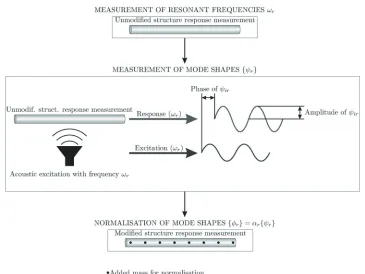
The basic idea of the tuned-sinusoidal method is presented in Fig. 1. First, the response of the structure, excited by an unknown force, is measured. Different excitation techniques, such as sound excitation, impact excitation, etc., can be used, as long as the spectral density of the excitation is constant across the whole frequency range of the measurement (white-noise excitation). The resonant frequencies ωr are on the peaks of the measured frequency spectrum. Next, the mode shapes {ψr} are measured. The structure is subjected to the acoustic excitation (with a loudspeaker) and only the response of the individual point on the structure is measured. If the structure is acoustically excited with a sine that is tuned to the resonant frequency ωr, then the structure will respond with an ODS, that can be used as an un-normalised mode shape {ψr}, as shown by Schwarz and Richardson [10]. This assumption is valid because the mode shape that corresponds to the frequency
ωr prevails over all the other mode shapes in the
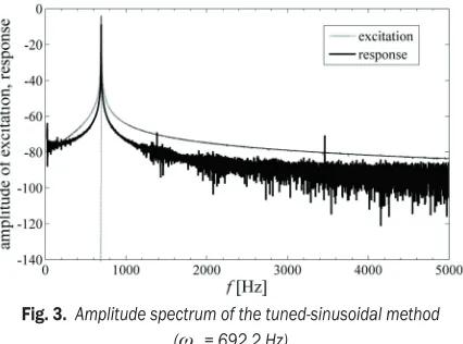
response of the structure. Therefore, the response of the structure is almost a pure sine with a frequency ωr, as shown in Figs. 2 and 3.
Fig. 2. Time signal of the tuned-sinusoidal method (ωr = 692.2 Hz)
The structure needs to be excited with all the individual resonant frequencies ωr and the responses
at all the points of the structure need to be measured for each resonant frequency. The amplitude of the excitation is not of significant importance; it only needs to be equal for all the measurements and the response needs to be within the measurement range
of the LDV. Besides the response of the structure,
the signal that is sent to the loudspeaker for the excitation is also measured. The phase between the sine of the excitation and response signal is used as a phase of individual component ψir of the mode shape {ψr}. The actual phase between the excitation and the response is different from the measured phase, because the sound has to travel from the loudspeaker to the structure (the influence of the damping on the resonant frequency is neglected). However, to define the un-normalised mode shapes, only the relative relations between the phases of the individual points on the structure are needed. This is especially so when the proportional damping is presumed and the mode shapes are not complex (the phase is either 90
or –90°). The amplitude of the response sine signal defines the amplitude of the individual component ψir of the mode shape {ψr}. Therefore, the structure has to be excited and the response needs to be measured for every (ith) measurement point at all the resonant frequencies ωr to obtain the amplitude and phase of each component ψir.
Fig. 3. Amplitude spectrum of the tuned-sinusoidal method (ωr = 692.2 Hz)
continues until the last resonant frequency in the frequency range of the measurement. This procedure is repeated for all the measurement points and the un-normalised mode shapes {ψr} are defined. The name tuned-sinusoidal method is used for the described method since the acoustic sine excitation is tuned to the measured resonant frequencies. The support of the structure can be free-free or fixed. The free-free support is usually more desirable for the comparison with the numerical model.
1.1 Mass-Normalisation of the Measured Mode Shapes
The measured mode shapes {ψr} are not mass normalised since the excitation force is not measured when performing the tuned-sinusoidal method. Therefore, the method presented by Parloo et al. [4] that enables the mass-normalisation of the operational mode shapes was used. It works on the basis of the modal sensitivity of the structure. The main idea of Parloo’s method is to normalise the measured mode shapes by multiplying them with scaling factors. A known mass is added to the selected points of the structure to change the resonant frequencies. The scaling factors are calculated from these changes by using the sensitivity analysis. The term mass-change strategy is frequently used to denote this method.
Other researchers also analysed the use of modal sensitivity to mass-normalise the operational mode shapes. Lopez-Aenlle et al. [11] to [14], Fernandez et al. [15] and [16] and Coppotelli [17] gave suggestions about how to accurately normalise the mode shapes using different types of mass-change strategies.
Lopez-Aenlle et al. [11] analysed the equations for the calculation of the scaling factors and developed an iterative procedure for better accuracy. In [14] and [15] Lopez-Aenlle et al. and Fernandez et al. analysed and experimentally verified the influence of the location, number and size of the added masses on the accuracy of the results. Additional instructions on how to perform accurate calculations of the scaling factors were given by Lopez-Aenlle et al. in [13].
The modal sensitivity of the rth resonant frequency ωr and the mode shape {ψr} are defined in [18], as shown in Eqs. (1) and (2), where pj represents one of the Np structural modifications.
∆ωr ωr
j j N j p p p 2 2 1 = ∂ ∂ =
∑
, (1)∆{ }φr { } .φ j j N j r p p p = ∂ ∂ =
∑
1 (2)Modal sensitivity describes the influence of the structural modifications on the modal parameters of the structure.
The mass-change strategy is based on Eq. (1), as shown by Parloo et al. [4]. If the structural modifications pj are the changes of mass at different points of the structure, then they can be described by
a change of the mass matrix [∆M]. A known mass
[∆M] needs to be added to the structure to perform the mass-change strategy. The change of the mass matrix causes a variation of the modal parameters. If the modal parameters of the unmodified and modified structures are measured, then the scaling factors αrcan be calculated as shown in Eq. (3):
α ω ω
ω ψ ψ
r r r M
r M r T M r
= ( − )
{ } [ , ]{ },
,
2 2
2 ∆ (3)
where ωr denotes the rth resonant frequency of the unmodified structure and ωr,M is the rth resonant frequency of the modified structure (when the mass
[∆M] is added). {ψr} is the un-normalised mode shape of the structure. A detailed derivation of Eq. (3) can be found in [4] and [11], where a presumption is made that the mode shapes do not change significantly when adding the mass to the structure ({ψr} ≈ {ψr,M}). When this presumption is valid, accurate scaling factors αr can be calculated from Eq. (3) and the mode shapes of the modified structure {ψr,M} can be used for the calculation of scaling factors instead of {ψr}, as shown by Lopez-Aenlle et al. [11].
When the presumption {ψr} ≈ {ψr,M} is not valid,
it is advisable to use the Bernal projection equation
[19] that gives good estimates of the scaling factor αr even in cases when the mode shapes change significantly during the normalisation procedure. The
Bernal projection equation is shown in Eq. (4):
α ω ω
ω ψ ψ
r r r M rr r M r T r M
B M = ( − ) { } [ , ]{ }, , , 2 2
2 ∆ (4)
where Brr represents the rth diagonal element of the
matrix [B]. The matrix [B] is calculated as shown in Eq. (5), where [Ψ] denotes the modal matrix of the
unmodified mode shapes {ψr} and [ΨM] the modal matrix of the modified mode shapes {ψr,M}:
[ ] [ ] [B = Ψ −1 ΨM]. (5)
by multiplying the un-normalised mode shapes {ψr} by αr:
{ }φr =α ψr{ }.r (6)
2 EXPERIMENT AND NUMERICAL MODEL
2.1 Sample
A sample with the proper geometrical and modal properties was needed to compare the experimental and numerical results. Therefore, a small steel beam with a rectangular cross-section (1.94×20.2 mm) was used (Fig. 4). The beam was 121.42 mm long and had a mass of 37 grams. The geometrical parameters are not rounded to integers, because the dimensions of the sample were measured with a calliper to ensure greater accuracy of the numerical model’s results. A total of 13 points, denoted with the numbers 0 to 12, were used for the measurement, as shown in Fig. 4. The results of the numerical model were calculated for the same 13 points. Only the bending mode shapes in the direction of the shorter side of the cross-section (1.94 mm) were measured; however, all the other mode shapes can be measured in a similar manner.
Fig. 4. The sample that was used for the measurements and to build the numerical model
2.2 Numerical Model
A numerical finite-element method (FEM) model was built with commercial software (Ansys). The model was based on the geometrical and material parameters (density, modulus of elasticity, Poisson’s ratio [20]) of the sample. A numerical modal analysis was performed on the model to determine the resonant frequencies and the normalised mode shapes. Since the damping is based on the results of the measurement, it is reasonable to use only the resonant frequencies and mode shapes for the comparison with the experimental results. The results of the model are relatively accurate, because the structure is homogeneous and without any joints or other sources of non-linearity [21] and [22].
2.3 Experimental Procedure
First, the response of the structure to impulse excitation was measured. The impact excitation was carried out using a small steel ball (4 mm diameter, 0.26 grams weight) that was glued to a string and swung into the structure at all the measurement points to ensure that all the mode shapes were excited well. The resonant frequencies ωr were determined from the peaks of the frequency spectrum of the response.
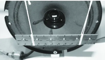
The structure was then acoustically excited with the loudspeaker and the un-normalised mode shapes ψr were defined from the response of the structure, as described in Section 1. The experimental set-up is shown in Fig. 5. A 6-W loudspeaker with a wide frequency range was used to excite the structure and the response of the structure was measured with a Polytec PDV-100 LDV. The frequency range of the LDV is from 0.5 Hz to 22 kHz and the sensitivity was set to 100 mm/s.
For the normalisation of the mode shapes with the mass-change strategy, six magnets, each with a mass of 0.21 grams, were added at points 1, 3, 5, 7, 9 and 11 on the structure and the resonant frequencies ωr,M of the modified structure were measured using impact excitation (with a steel ball). Then the scaling factors αr were calculated, as described in Section 1.1, and finally the normalised mode shapes ϕr were defined (ϕr = αr · ψr).
Fig. 5. Experimental set-up for the tuned-sinusoidal method
3 RESULTS OF THE NUMERICAL MODEL AND THE EXPERIMENTAL PROCEDURE
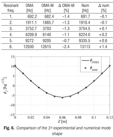
Table 1 presents the experimental and numerical resonant frequencies. OMA denotes the measured resonant frequencies ωr before the mass was added to the structure for the mass-change strategy and OMA-M denotes the resonant frequencies ωr,M after the mass was added to the structure. The numerical (num) and experimental (OMA) resonant frequencies
differ by less than 1.5% (∆ num), and the first four by
even less than 0.3%. Therefore, it was concluded that the measurements of the resonant frequencies were accurate.
After the mass is added to the structure for the mass-change strategy the resonant frequencies
reduce by about 0.7 to 2.4% (∆ OMA-M). This is a
relatively small change for the mass-change strategy [13]; however, it still ensures the accurate mass normalisation of the mode shapes ψr.
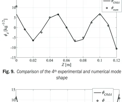
Figs. 6 to 11 show the mass-normalised mode shapes that were measured with the tuned-sinusoidal method (ϕOMA) and calculated with a numerical FEM model (ϕnum). It is clear that the experimental mode shapes are in good agreement with the numerical mode shapes. This agreement proves that not only the shape of the mode shapes, but also the normalisation (the scaling factor), was accurately measured.
The correlation between the experimental and the numerical mode shapes was calculated using the modal assurance criterion (MAC), which is described in detail in [18], [23] and [24]. The result of the MAC procedure is a matrix with real values between 0 and 1. The value of each element of the MAC matrix belongs to a pair of mode shapes and describes their correlation (a higher value means a better correlation). The diagonal values of the MAC matrix are equal to 1 and the non-diagonal to 0 in the ideal case (when the numerical and experimental mode shapes are in perfect correlation). The MAC results are shown in Fig. 12. All the diagonal values of the MAC matrix are close to 1 (higher than 0.96) and the non-diagonal values are close to 0 (the highest is 0.12). The MAC results prove that the mode shapes were measured well, because there is a clear correlation between the numerical and the experimental mode shapes.
Table 1. Comparison of the resonant frequencies calculated with the numerical model (num) and measured with the
tuned-sinusoidal method (OMA)
Resonant
freq. OMA [Hz] OMA-M [Hz] ∆ OMA-M [%] Num [Hz] ∆ num [%]
1. 692.2 682.4 –1.4 691.7 –0.1
2. 1911.1 1885.7 –1.3 1910.4 –0.1
3. 3752.7 3703 –1.3 3754.5 +0.1
4. 6209.9 6140 –1.1 6224.0 +0.2
5. 9272 9205 –0.7 9335.5 +0.6
6. 12930 12615 –2.4 13113 +1.4
Fig. 6. Comparison of the 1st experimental and numerical mode shape
Fig. 7. Comparison of the 2nd experimental and numerical mode shape
Fig. 9. Comparison of the 4th experimental and numerical mode shape
Fig. 10. Comparison of the 5th experimental and numerical mode shape
Fig. 11. Comparison of the 6th experimental and numerical mode shape
Fig. 12. MAC correlation of the experimental and the numerical
mode shapes
4 CONCLUSION
An innovative, non-contact method for the modal analysis of small and light structures was presented. The method is based on an acoustic sine excitation that is tuned to individual resonant frequencies. A single response measurement (with an LDV) is needed to determine the resonant frequencies and the un-normalised mode shapes. A mass-change strategy is used to calculate the scaling factors for the normalisation of the mode shapes.
The tuned-sinusoidal method gives good results on the sample that was used in this study. The resonant frequencies are measured accurately and differ from the results of the numerical model by less than 1.5% in a wide frequency range (up to 15 kHz). The first six bending-mode shapes were also measured well, which was confirmed by the MAC analysis. The good agreement between amplitudes of the experimental and the numerical mode shapes confirms that the scaling factors for the mass-normalisation of the measured mode shapes were correctly defined. It can, therefore, be concluded that the tuned-sinusoidal method gives accurate results for simple small and light structures.
The tuned-sinusoidal method has some clear advantages compared to other methods used for the modal analysis of small and light structures. It is a non-contact method (the contact is only needed if the mass-normalisation is to be performed), which is very convenient, because the sensors do not add any mass to the measured structure and therefore do not affect the results of the modal analysis. The presented method is also very practical, because a single response is measured and the experimental set-up is very simple and effective. The whole structure (not just a single point) is subjected to acoustic excitation; therefore, all the measured mode shapes are excited well. An important advantage of the presented method compared to similar methods is that the mode shapes are better accentuated (due to sine excitation), which can improve measurements on small and light structures, where the response of the structure is relatively weak. The better accentuation of the mode shapes is achieved because all the excitation energy is concentrated at just a single mode and all the other modes are not excited.
makes the tuned-sinusoidal method more appropriate for smaller structures, because the excitation intensity can be too low to excite larger structures.
5 REFERENCES
[1] Brincker, R, Möller, N. (2006). Operational modal
analysis - a new technique to explore. Sound and
Vibration, vol. 40, no. 6, p. 5-6.
[2] Devriendt, C., Guillaume, P., Reynders, E, De Roeck, G. (2007). Operational modal analysis of a bridge using transmissibility measurements. Proceedings of IMAC-25: A Conference and Exposition on Structural
Dynamics, p. 748-757.
[3] Parloo, E., Guillaume, P., Anthonis, J., Heylen,
W., Swevers, J. (2003). Modelling of sprayer
boom dynamics by means of maximum likelihood identification techniques, Part 1: A comparison of input-output and output-only modal testing. Byosistems
Engineering, vol. 85, no. 2, p. 163-171, DOI:10.1016/
S1537-5110(03)00044-8.
[4] Parloo, E., Verboven, P., Guillaume, P., Van Overmeire, M. (2002). Sensitivity-based operational mode shape normalisation. Mechanical Systems and Signal
Processing, vol. 16, no. 5, p. 757-767, DOI:10.1006/
mssp.2002.1498.
[5] Siringoringo, D.M., Fujino, Y. (2009). Noncontact operational modal analysis of structural members by laser Doppler vibrometer. Computer-aided Civil and
Infrastructure Engineering, vol. 24, no. 4, p. 249-265,
DOI:10.1111/j.1467-8667.2008.00585.x.
[6] Ahmida, K.M., Ferreira, L.O.S. (2004). Design and modeling of an acoustically excited double-paddle scanner. Journal of Micromechanics and
Microengineering, vol. 14, no. 10, p. 1337-1344,
DOI:10.1088/0960-1317/14/10/007.
[7] Xu, Y. F., Zhu, W.D. (2011). Operational modal analysis of a rectangular plate using noncontact acoustic excitation. Rotating Machinery, Structural Health Monitoring, Shock and Vibration, Vol. 5 (Conference Proceedings of the Society for Experimental
Mechanics Series). Springer, New York, p. 359-374,
DOI:10.1007/978-1-4419-9428-8_30.
[8] Devriendt, C., Guillaume P. (2008). Identification of modal parameters from transmissibility measurements.
Journal of Sound and Vibration, vol. 314, no. 1-2,
p. 343-356, DOI:10.1016/j.jsv.2007.12.022.
[9] Devriendt, C., De Sitter, G., Vanlanduit, S., Guillaume, P. (2009). Operational modal analysis in the presence of harmonic excitations by the use of transmissibility measurements. Mechanical Systems and Signal
Processing, vol. 23, no. 3, p. 621-635, DOI:10.1016/j.
ymssp.2008.07.009.
[10] Schwarz, B.J., Richardson, M.H. (2004). Measurements
required for displaying operating deflection shapes.
Proceedings of IMAC-22: A Conference on Structural
Dynamics, p. 701-706.
[11] Lopez-Aenlle, M., Brincker, R., Fernandez-Canteli, A.,
Garcia, L.M.V. (2005). Scaling-factor estimation by the mass-change method. Proceedings of IOMAC-1, p. 53-64.
[12] Lopez-Aenlle, M., Brincker, R., Fernandez-Canteli,
A. (2005). Some methods to determine scaled mode shapes in natural input modal analysis. Proceedings
of IMAC-23: A Conference on Structural Dynamics,
p. 141-145.
[13] Lopez-Aenlle, M., Fernandez, P., Brincker, R.,
Fernandez-Canteli, A. (2010). Scaling-factor estimation using an optimized mass-change strategy (Correction of: vol. 24, no. 5, p. 1260-1273, 2010). Mechanical
Systems and Signal Processing, vol. 24, no. 8, p.
3061-3074.
[14] Lopez-Aenlle, M., Fernandez, P., Brincker, R.,
Fernandez-Canteli, A. (2007). Scaling-factor estimation using an optimized mass-change strategy, Part 1: Theory. Proceedings of IOMAC-2, p. 421-428.
[15] Fernandez, P., Lopez-Aenlle, M., Garcia, L.M.V.,
Brincker, R. (2007). Scaling-factor estimation using an
optimized mass-change strategy, Part 2: Experimental Results. Proceedings of IOMAC-2, p. 429-436.
[16] Fernandez, P., Reynolds, P., Lopez-Aenlle, M. (2011). Scaling mode shapes in output-only systems by a consecutive mass change method. Experimental
Mechanics, vol. 51, no. 6, p. 995-1005, DOI:10.1007/
s11340-010-9400-0.
[17] Coppotelli, G. (2009). On the estimate of the FRFs from operational data. Mechanical Systems and Signal
Processing, vol. 23, no. 2, p. 288-299, DOI:10.1016/j.
ymssp.2008.05.004.
[18] Maia, N.M.M., Silva, J.M.M. (1997) Theoretical and
Experimental Modal Analysis, 1st ed. Research Studies
Press, John Wiley and Sons, Taunton, New York, etc.
[19] Bernal, D. (2004). Modal scaling from known mass
perturbations. Journal of Engineering Mechanics, vol. 130, no. 9, p. 1083-1088, DOI:10.1061/(ASCE)0733-9399(2004)130:9(1083).
[20] Kraut, B., Puhar, J., Stropnik, J. (2003) Krautov
strojniški priročnik (Kraut’s Engineering Handbook),
14th ed., Littera picta, Ljubljana. (in Slovene)
[21] Čermelj, P., Boltežar, M. (2006). Modelling localised
nonlinearities using the harmonic nonlinear super model. Journal of Sound and Vibration, vol. 298, no. 4-5, p. 1009-1112, DOI:10.1016/j.jsv.2006.06.042. [22] Čelič, D., Boltežar, M. (2008). Identification of the
dynamic properties of joints using frequency-response functions. Journal of Sound and Vibration, vol. 317, no. 1-2, p. 158-174, DOI:10.1016/j.jsv.2008.03.009. [23] Allemang, R.J. (2003). The modal assurance criterion
- Twenty years of use and abuse. Sound and Vibration, vol. 37, no. 8, p. 14-23.
[24] Fotsch, D., Ewins, D.J. (2000). Application of MAC
in the Frequency Domain. Proceedings of IMAC-18: A