STAGE-DISCHARGE MODELING USING SUPPORT VECTOR MACHINES

STAGE-DISCHARGE MODELING USING SUPPORT VECTOR

MACHINES

Department of Civil Engineering, National Institute of Technology, Kurukshetra, 136119, Haryana (India), Fax: +911744238050

[email protected], [email protected]

*Corresponding Author

(Received: January 13, 2010 – Accepted in Revised Form December 15, 2011)

doi:10.5829/idosi.ije.2012.25.01a.01

Abstract Establishment of rating curves are often required by the hydrologists for flow estimates in the streams, rivers etc. Measurement of discharge in a river is a time-consuming, expensive, and difficult process, and the conventional approach of regression analysis of stage-discharge relation does not provide encouraging results especially during the floods. Present study is aimed at the application of support vector machines (SVMs) based algorithm for modelling stage-discharge relation including the hysteresis effect. A data set of two discharge-measuring stations located on two Indian rivers has been used for analysis in the present study. A back propagation neural network model was employed in order to compare the performance of the results based on support vector machines based modelling technique. The outcome of the study suggests that the support vector machines works well for both the data sets and produce promising results in comparison to the neural network technique. Finally, the results also suggest the suitability of SVMs algorithm in predicting the looped rating curve having hysteresis effect.

Keywords Rating curve; Hysteresis modelling; Neural network; Support vector machines.

ﺖﺳا و شور فرﺎﻌﺘﻣ ﺰﯿﻟﺎﻧآ ر نﻮﯿﺳﺮﮔ ﻪﻄﺑار ﻪﻠﺣﺮﻣ ﻪﯿﻠﺨﺗ هﺪﻨﻨﮐ مﺮﮕﻟد ﺞﯾﺎﺘﻧ يا هﮋـﯾو ﻪـﺑ رد نﺎـﻣز ﻪـﺋارا ﻞﯿـﺳ ﯽﻤﻧ ﺪﻫد . ﺮﺿﺎﺣ ﻪﻌﻟﺎﻄﻣ ﺎﺑ فﺪﻫ ﺑ ﻪ زا يﺮﯿﮔرﺎﮐ ﻦﯿﺷﺎﻣ يرادﺮﺑ نﺎﺒﯿﺘﺸﭘ ) SVMs ( ﺮﺑ ﯽﻨﺘﺒﻣ ﯽﻤﺘﯾرﻮﮕﻟا ياﺮﺑ لﺪﻣ يزﺎﺳ ﻪﻄﺑار ﻪﻠﺣﺮﻣ ﻪﯿﻠﺨﺗ ﻦﺘﻓﺮﮔ ﺮﻈﻧ رد ﺎﺑ ﺮﺛا

ﺴﭘ ﺖﺳا ﻪﺘﻓﺮﮔ ترﻮﺻ ﺪﻧﺎﻤ .

هداد يﺮﺳ ﮏﯾ زا ﺑ ﻪ آ ﺖـﺳد زا هﺪـﻣ ود هﺎﮕﺘﺴﯾا هزاﺪﻧا يﺮﯿﮔ رد ﻊﻗاو ﻪﯿﻠﺨﺗ ﻪﻧﺎﺧدور ود

يﺪﻨﻫ ياﺮﺑ رد ﺰﯿﻟﺎﻧآ ﺮﺿﺎﺣ ﻪﻌﻟﺎﻄﻣ ﺖﺳا هﺪﺷ هدﺎﻔﺘﺳا

. لﺪﻣ زا رﺎﺸﺘﻧا ﺲﭘ رﻮﺧ ﻪﮑﺒﺷ ﯽﺒﺼﻋ رﻮﻈﻨﻣ ﻪﺑ دﺮﮑﻠﻤﻋ ﻪﺴﯾﺎﻘﻣ ﺞﯾﺎﺘﻧ سﺎﺳا ﺮﺑ ﻦﯿﺷﺎﻣ يرادﺮﺑ نﺎﺒﯿﺘـﺸﭘ ، ﯽـﻨﺘﺒﻣ ﺮـﺑ شور لﺪﻣ ﺳ ﺖﺳا هﺪﯾدﺮﮔ هدﺎﻔﺘﺳا يزﺎ . ﻪﺠﯿﺘﻧ ﻪﻌﻟﺎﻄﻣ نﺎﺸﻧ ﯽﻣ ﺪﻫد ﻦﯿﺷﺎﻣ ﻪﮐ يرادﺮﺑ نﺎﺒﯿﺘـﺸﭘ ياﺮـﺑ ود ﺮـﻫ ﻪـﻋﻮﻤﺠﻣ هداد و هدﺮﮐ ﻞﻤﻋ ﯽﺑﻮﺧ ﻪﺑ ﺎﻫ هﺪﻨﻨﮐ راوﺪﯿﻣا ﺞﯾﺎﺘﻧ

يا رد ﺎﺑ ﻪﺴﯾﺎﻘﻣ ﮏﯿﻨﮑﺗ ﻪﮑﺒﺷ ﯽﺒـﺼﻋ ـﺑ ﻪ آ رﺎـﺑ ﺖـﺳا هدرو . رد ﺖﯾﺎﻬﻧ ، ﯽﮐﺎﺣ ﻦﯿﻨﭽﻤﻫ ﺞﯾﺎﺘﻧ زا ندﻮﺑ ﺐﺳﺎﻨﻣ ﻢﺘﯾرﻮﮕﻟا SVMs رد ﺶﯿﭘ ﯽﻨﯿﺑ ﯽﻨﺤﻨﻣ ﯽﺑﺎﯾزرا ﻪﻘﻠﺣ يا ﺎﺑ ﺮﺛا ﺲـﭘ -1. INTRODUCTION

Prediction of stage-discharge relation or a rating curve is of immense importance for reliable planning, design and management of most of the projects on water resources. A common practice is to measure the river stages at regular intervals and use them for further discharge calculations, which can be used for future hydrological analysis. The stage and discharge at a gauging site is generally represented by a rating curve. The rating curve is determined by assuming that there exists a unique

relation between stage and discharge of the river at the given site. However, the stage-discharge relationship is time dependent and often exhibits a random phenomenon with fluctuations. The process of establishing a rating curve can be assumed to be a mapping problem wherein stage is considered as the input variable and discharge is the output variable. Mostly, a power equation is used to establish the relation between stage and discharge whose variables can be determined by regression analysis. A major limitation of this approach is that it is not able to take into account

A.Goel* and M. Pal

ﺎـﻫﻪﻧﺎﺧدور و ﺮﻬﻧ رد نﺎﯾﺮﺟ ﻦﯿﻤﺨﺗ ياﺮﺑ ﺐﻠﻏا ﺎﻫﺖﺴﯾژﻮﻟورﺪﯿﻫ ﻂﺳﻮﺗ ﯽﺑﺎﯾزرا يﺎﻫﯽﻨﺤﻨﻣ دﺎﺠﯾا

هﺪﯿﮑﭼ

راﻮﺷد و ﻪﻨﯾﺰﻫﺮﭘ ،ﺮﯿﮔﺖﻗو ﺪﻨﯾاﺮﻓ ﮏﯾ ﻪﻧﺎﺧدور ﮏﯾ رد ﻪﯿﻠﺨﺗ ﻪﺑ طﻮﺑﺮﻣ ﺮﯾدﺎﻘﻣ يﺮﯿﮔهزاﺪﻧا .ﺪﺷﺎﺑﯽﻣ زﺎﯿﻧ درﻮﻣ

the hysteresis effect, i.e. two distinct discharges occur for the same stage, one during the rising river stage, which is a higher value, and another during recession, which is a lower value.

Recently, there has been a growing interest in the analysis of the complex hydrological processes by using modelling techniques like artificial neural networks [1]. Any hydrological system consists of nonlinear and multivariate variables, which may have unknown relationships among them. The artificial neural networks (ANN) adapt itself to reproduce the desired output when presented along with input data sets. Several studies have reported the application of neural network in predicting the stage-discharge curve [2-8]. Most of the studies employing neural networks have used back propagation and radial basis function types of neural networks to establish the stage-discharge relationship. A neural network based modelling approach requires setting up several user-defined parameters like learning rate, momentum, optimal number of nodes in the hidden layer and the number of hidden layers, so as to have a less complex network with a relatively better generalization capability. Further, training a neural network requires a number of iterations and a large number of training iterations may force ANN to over train, which may affect the predicting capabilities of the model. Keeping in view these limitations of ANN, and the recent use of SVMs in water resource studies [9-14], this study explores the potential of support vector machines in predicting the rating curve development using data from two different gauging sites of two Indian rivers. The performance of support vector machines is compared with a back propagation neural network modelling approach for both data sets.

2. SUPPORT VECTOR MACHINES

Support vector machines (SVMs) are classification and regression methods, which have been derived from statistical learning theory [15]. The SVMs classification methods are based on the principle of optimal separation of classes. If the classes are separable – this method selects, from among the infinite number of linear classifiers, the one that minimize the generalization error, or at least an upper bound on this error, derived from structural

risk minimization. Thus, the selected hyper plane will be one that leaves the maximum margin between the two classes, where margin is defined as the sum of the distances of the hyper plane from the closest point of the two classes [15]. The Support Vector Machines can also be applied to regression problems and can be formulated as given below.

Vapnik proposed -Support Vector Regression (SVR) by introducing an alternative - the Insensitive Loss Function. This loss function allows the concept of margin to be used for regression problems. The purpose of the SVR is to find a function having at most deviation from the actual target vectors for all given training data and have to be as flat as possible [16]. This can be put in other words as the error on any training data has to be less than



; which is negligible. For a given training data with k number of samples, represented by



x , y ,..., x , y1 1





k k



_{, a linear} decision function can be represented by:

 

where _{w R} N _{and b}



_{R. w,x represents the dot} product in space _RN_{. A smaller value of w} indicates the flatness of equation 1, which can be achieved by minimising the Euclidean norm as

defined by w2[16]. Thus, an optimisation

problem for regression can be written as:

Minimise 1 2

w 2

i i

i i

y w,x -b w,x +b - y

 

  

 

 

The optimisation problem in Equation 2 is based on the assumption that there exists a function that provides an error on all training pairs which is less than



. In real life problems, there may be a situation like one defined for classification by [17]. So, to allow some more error, slack variables _{ ,} '

can be introduced and the optimisation problem defined in Equation 2 can be written as:

Minimise



'



1

k 2

i i

i

1 w + C

2



_  

Subject to

'

i i i

i i i

y w,x - b

w,x +b - y

   

   

 

 

 (3)

f x,a = w,x +b (1)

and _, '

i i 0

   for all i = 1, 2,……, k.Parameter

C is determined by the user and it decides the trade-off between the flatness of the function and the amount by which the deviations to the error more than



can be tolerated. The optimisation problem in Equation 3 can be solved by replacing the inequalities with a simpler form determined by transforming the problem to a dual space representation using Lagrangian multipliers [18]. The prediction problem in Equation 1 can now be written as:







'



1

,

k

i i i

i

f x    x ,x +b







 (4)

where λ_iand λ_i'are positive Lagrange multipliers. The techniques discussed above can be extended to allow for non-linear support vector regression by introducing the concept of the kernel function [15]. This is achieved by mapping the data into a higher dimensional feature space, thus performing linear regression in feature space. The regression problem in feature space can be written by replacing x xi j with Φ x

 

i ×Φ x

 

j .

where K x ,x



_{i j}



Φ x

 

_i ×Φ x

 

_j

Regression function for this case can now be written as:







'







1

,

k

i i i

i

f x   K x , x +b







 (5)

3. APPLICATION OF SVMS FOR STAGE-DISCHARGE PREDICTION

To assess the usefulness of SVMs based modelling approach in predicting the stage-discharge relationship, the data sets collected on two gauging sites located on river Brahmani and Mahanadi in Orrissa (India) was used (Table 1).

A hypothetical data set consisting of 168 pairs exhibiting the hysteresis effect was also created for studying the loop-rating curve in order to judge the performance of SVMs in the flooding state of flow to account for the hysteresis effect. The stage values and the corresponding discharge were taken at an interval of 0.1 m, starting as the initial stage value from 100.0 m for rising as well as falling stages.

The SVMs are used in calculating correlation

coefficients and root mean square errors (RMSE) by using cross-validation to generate the model on the input data set and predicting the discharge for both data sets with different input combinations. The cross-validation is a method of estimating the accuracy of a classification or regression model. The input data set is divided into several parts (a number defined by the user), with each part in turn used to test a model fitted to the remaining parts. For this study, a ten-fold cross-validation was used. The use of SVMs requires setting of the user-defined parameters such as regularisation parameter (C), type of kernel and kernel specific parameters. As the choice of kernel may influence the prediction capabilities of the SVMs, present study uses a polynomial (





_{x y +1}





d_{) and a radial}

basis kernel (e-γ x- y2) where d and  are kernel specific parameters. The suitable value of parameters C, d and  (Table 2) were obtained by comparing the correlation coefficients and root mean square error (RMSE) values after a number of trials for the different data sets used in the present study.

TABLE 1. Details of the gauging sites with number of data set (1440 pairs)

Name of River

Name of Site

Drainage area (sq

km)

Site number

Months and years of observations

Brahmani Jenapur 33955 61N June, July, August,

September and October, 1981 to 1986

Mahanadi Tikarapara 124450 44 June, July, August,

September and October, 1981 to 1986

TABLE 2.Values of user defined parameters used with SVMs for different data sets

Gauging site/Data Polynomial kernel_{C d} RBF kernel_{C }

Jenapur site 5 1 5 0.6

Tikarapara site 1 1 1 1.2

Hypothetical data 5 1 5 0.6

4. MODEL DEVELOPMENT AND PERFORMANCE CRITERIA

on Brahmani river and Tikarapara (1440 pairs) on Mahanadi river in Orrisa (India) have been used in the present study. A hypothetical data set of stage and discharge (168 pairs) showing hysteresis effect on the rating curve was also used. To model the rating curves, seven combinations of stage and discharge values were considered as input parameters for the Jenapur as well as Tikarapara site. Tables 3 and 4 provide the list of all input variable used to predict the discharge for both sites, where S_trepresents the stage at any time t (i.e. month of August for each year in present study) and Q_tis the corresponding discharge. Further, S_t₂,S_t₁,S_t₁,S_t₂ and Qt2,Qt1,Qt1,Qt2

represent stages and discharges at (t-2), (t-1), (t+1) and (t+2) times respectively i.e. months of June, July, Sept and October for each year. Normalisation of the data was carried out so as to bring all input variables within a range of 0 to 1. Correlation coefficient and root mean square error (RMSE) values for different data sets (Tables 3 & 4) are used for the performance evaluation of the models and comparison of the results for establishing the stage-discharge curve using SVMs. A higher value of correlation coefficient with a smaller value of RMSE for given set of input parameters is considered to be a better performing model. To study the scatter, a line of perfect agreement (i.e. a line at 45 degrees) was plotted in the resulting graphical output between the actual and the predicted discharge values with both data sets. Further, rating curves were also plotted for the predicted and actual discharges at different stages.

5. ANALYSIS AND DISCUSSION OF RESULTS

Much success has already been achieved by using modelling techniques like Artificial Neural Network (ANN) in stage-discharge analysis and an exhaustive literature review indicates that so far no works have reported the use of support vector machines based approach for the prediction of the rating curve. One major advantage of using SVMs modelling approach is the use of quadratic optimization problem, which provides global minima in comparison to the presence of local minima due to the use of a non-linear optimization

problem with a back propagation neural network approach. Further, the SVMs require setting of fewer user-defined parameters. The SVMs, in addition to the choice of kernel, require setting up of kernel specific parameters. The optimum values of the regularization parameter C and the size of the error-insensitive zone  need to be determined. After several trials by varying the value of error-insensitive zone for a fixed value of C and kernel specific parameter, a value of 0.0010 was found to be working well for different data sets used in this study. User-defined parameters



C,d,



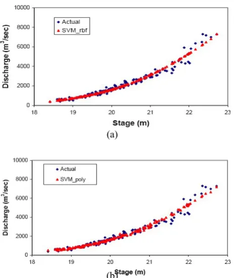
working well for SVMs modelling technique with different data sets in the present work are given in Table 2.

5.1 Jenapur Data Set The results of the RBF and polynomial kernel based SVMs (SVM_rbf and SVM_poly) for each data set for Jenapur site in terms of correlation coefficients and RMSE are given in Table 3. For each combination of inputs, the values of kernel specific parameters d and  that provide the minimum RMSE and maximum correlation coefficient using a 10 fold cross validation were used. The value of regularization parameter (C) was kept equal with same input data combination using both kernels. Figures 1(a) and 1(b) provide the rating curves obtained by using RBF and polynomial kernels respectively in comparison to the actual values. These curves are plotted for the data set providing the highest value of the correlation coefficient and the minimum value of RMSE. With the RBF kernel, the highest value of correlation coefficient (i.e. 0.988) and Minimum value of RMSE (249.02) were obtained using a data set consisting of S_t as the input

parameter. The input combination of

1 1

,

t t t

presented in Figure 3(a), while Figure 3(b) represents the variation of actual and predicted discharges with time. It is evident from Figure 3(a) that errors for most of the points are within a range of



250 m3/sec with the RBF kernel for all the stages and no major deviation of the results is observed for any discharge value. A comparison of the results in Figure 3(b) suggests almost perfect agreement between predicted and actual discharges with time.

(a)

(b)

Figure 1. Stage discharge relationship for actual and predicted values by (a) RBF kernel (b) polynomial kernel based SVMs for Jenapur site.

(a)

(b)

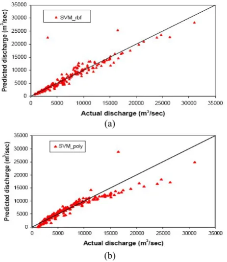
Figure 2.Actual versus predicted discharge by (a) RBF kernel (b) polynomial kernel based SVMs for Jenapur site.

Figure 3(a). Error in computed discharge with respect to observed discharge using RBF kernel based SVMs for Jenapur site.

TABLE 3. Values of correlation coefficient and root mean square error (RMSE) for different combinations of input parameters for Jenapur gauging site using support vector machines. The highlighted values indicate the best input combination.

Input parameters

error

t S

,S

S 0.972 380.93 0.949 572.08

, ,S Q

S 0.968 404.80 0.973 371.70

1 2 1, ,

, t t t

t S S Q

S 0.981 306.51 0.941 595.41

2 1 1 2 2, 1, 1, 2

t t t t t

t t t t

   

   

5.2. Tikarapara site data To validate the performance of the SVMs for stage-discharge prediction, another data set from Tikarapara gauging site on Mahanadi river (Table 1) was used. Seven combinations of input data as used for the Jenapur site were also tested for this site. The results are expressed in terms of correlation coefficients and RMSE and presented in Table 4. The optimal values of user-defined parameters C, d



4(a) and 4(b) provide the plot for actual and predicted discharges using a RBF and polynomial kernels based SVMs against the corresponding stage values for the best combination of input data set obtained from Table 4. Values for correlation coefficient of 0.934 and RMSE = 1929.80 were

achieved with input combinations of

1 1

, t t

t S and Q

S using RBF kernel as given in Table

4. The combination of

1 2

1  

 t t

t

t S S and Q

S , , provides the best

performance (i.e. correlation coefficient = 0.909 and RMSE = 2207.30) with the polynomial kernel based SVMs. The observed and estimated discharges obtained by using both the kernels are plotted in Figures 5(a) and 5(b). The perusal of these figures shows that there is a perfect correlation between observed and predicted discharge in RBF kernel based SVM. The results obtained for this data set suggest that SVMs modelling approach can effectively be used for

stage-discharge modelling. The results also suggest that RBF kernel works better for this data set.

(a)

(b)

Figure 4. Stage discharge relationship for actual and predicted values by (a) RBF kernel (b) polynomial kernel for Tikarapara site.

TABLE 4. Values of correlation coefficient and root mean square error (RMSE) for different combinations of input parameters for Tikarapara gauging site using support vector machines. The highlighted values indicate the best input combination.

Input parameters

RBF kernel Polynomial kernel Correlation

coefficient mean Root square error

Correlation coefficient mean Root

square error

t

S 0.928 2042.04 0.905 2268.85

1

, _t

t S

S 0.934 1934.63 0.908 2216.64

1 1,

, _{t t}

t S Q

S 0.934 1929.80 0.909 2212.87

1 2 1, ,

, t t t

t S S Q

S 0.933 1937.12 0.909 2207.39

2 1 2 1, , ,

, _{t t t t}

t S S Q Q

S 0.931 1970.82 0.908 2219.06

2 1 2 1, , ,

, t t t t

t S S Q Q

S 0.920 2081.94 0.905 2279.58

2 1 1 2

2 1 1 2

, , , , ,

, , ,

t t t t t

t t t t

S S S S S Q Q Q Q

       

0.926 2006.82 0.909 2225.36

and for this data set are given in Table 2. Figures

coefficient coefficient square error mean Correlation Root mean Correlation Root RBF kernel Polynomial kernel

0.988 249.02 0.950 567.34 square

0.984 286.54 0.945 583.51

0.987 260.28 0.937 609.99 0.987 257.59 0.950 576.89

S,S ,S ,Q ,Q

S,S ,S ,Q ,Q

t t1 t1

t t1

Q Q Q Q

t t1 t2 t1 t2

t t1 t2 t1 t2

(a)

(b)

Figure 5.Actual versus predicted discharge by (a) RBF kernel (b) polynomial kernel based SVMs. for Tikarapara site.

5.3. Comparison of SVM with back propagation neural network To compare the performance of SVMs with a neural network modelling approach, a back propagation neural network was used for both (Jenapur and Tikarapara) data sets. The input combinations providing the best results with RBF kernel based SVMs (Tables 3 and 4) were used in both data sets. After several trials, a three-layer network with one hidden layer having 8 nodes, a learning rate of 0.02, momentum value of zero and a total of 1000 iteration was found to provide the best results with both data sets (Table 5). Similar to the SVMs, a 10 fold cross-validation was used with neural network to get the results in term of correlation coefficient and RMSE values. The results from Tables 3 and 5 indicate that SVMs works equally well to the neural network modelling approach for Jenapur data set.

Figures 6(a) and 6(b) confirm the results obtained by a neural network modelling approach for this data set. For Tikarapara data set, a comparison of Tables 4 and 5 suggests a better performance by RBF kernel based SVMs algorithm in comparison

to a back propagation neural network approach. The rating curve as well as observed and estimated discharges obtained by using a back propagation neural network for Tikarapara data set are plotted in Figure 7(a) and 7(b). The results for both sites indicate an improved or comparable performance by SVMs approach (RBF kernel) for stage discharge modelling in comparison to the back propagation neural network algorithm.

TABLE 5. Values of correlation coefficient and root mean square error (RMSE) and obtained with back propagation neural network for both data sets (Jenapur & Tikarapara sites).

Data set

Back propagation neural network Correlation

coefficient

Root mean square error Jenapur data (S_tas input parameter) 0.988 248.97 Tikarapara data (

1 1

, t t

t S andQ

S as input

parameter) 0.919 2089.54

Figure 6(a).Stage discharge relationship for actual and predicted values by back propagation neural network for Jenapur site.

Figure 7(a).Stage discharge relationship for actual and predicted values by back propagation neural network for Tikarapara site.

Figure 7(b).Actual versus predicted discharge by back propagation neural network for Tikarapara site.

5.4 Looped-Rating Curve Modelling The SVMs approach was also employed to predict the discharge using a hypothetical data set in order to model a looped-rating curve. Two different data sets for rising and falling stages were created to judge the performance of SVMs for stage-discharge curve prediction. For both data sets, a 10-fold cross-validation was used to train and test the SVMs. The values of user-defined parameters obtained for this data set using both kernels are given in Table 2. The results obtained using both kernels are given in Table 6. A correlation coefficient value of nearly one indicates a good performance by using a RBF kernel SVMs approach for the looped-rating curve. Figure 8 provides a looped rating curve between actual and predicted discharges (RBF kernel based SVMs), suggesting almost a perfect match between actual and predicted discharge values except a slight deviation near the peak zone.

TABLE 6. Values of correlation coefficient and root mean square error (RMSE) obtained by SVMs using hypothetical data set.

Input parameters

RBF kernel Polynomial kernel Correlation

coefficient Root mean square

error

Correlation coefficient

Root mean square error

t

S(rising stage) 0.999 11.27 0.996 32.89

t

S(falling stage) 0.999 7.32 0.989 46.50

Figure 8. Loop rating curve obtained by using RBF kernel based SVMs along with the hypothetical data.

6. CONCLUSIONS

7. ACKNOWLEDGEMENTS

Authors are thankful to the Chief Engineer, Eastern gauging division, Bhuwneshwar (Orissa state), Central Water Commission, Ministry of Water Resources, Government of India for providing stage-discharge data, without which it would not have possible to complete the present study.

8. REFERENCES

1. ASCE task committee on application of ANNs in Hydrology, “Artificial neural networks in hydrology, II: hydrologic applications”, Journal of Hydraulic Engineering, ASCE, Vol. 5, (2000). No. 2, 124-137. 2. Tawfik, M., Ibrahim, A. and Fahmy, H., “Hysteresis

sensitive neural network for modelling rating curves”, Journal of Computing in Civil Engineering,Vol. 11, No. 3, (1997), 206–211.

3. Bhattacharya, B. and Solomatine, D.P., “Application of artificial neural network in stage discharge relationship”, Proceedings of 4th International Conference on Hydro informatics,(2000). Iowa, USA. 4. Jain, S. K. and Chalisgaonkar, D., “Setting up stage

discharge relations using ANN”, Journal of Hydrologic Engineering, Vol. 5, No.4, (2000), 428–433.

5. Sudheer, K. P. and Jain, S.K., “Radial basis function neural network for modelling rating curves”,Journal of Hydrologic Engineering, Vol 8, No.3, (2003), 161-164. 6. Olerleir, A.P., “Modelling stage discharge relationships

affected by hysterisis using the Jones formula and non linear regression”,Hydrological Sciences Journal, Vol. 51, No. 3, (2006), 365-388.

7. Bist, D.C.S., Raju, M.M. and Joshi, M. M., “ANN based river stage discharge modeling for Godavari river,

India”, Computer Modelling and New Technologies, Vol. 14, No. 3, (2010), 48-62.

8. Bist, D.C.S. and Jangid, A., “Discharge modeling using Adaptive neuro fuzzy inference system”, International Journal of Advanced Science and Technology, Vol. 31, (2011).

9. Pal, M. and Goel, A., “Prediction of the End depth ratio and discharge in semi circular and circular shaped channels using support vector machines”, Flow Measurement and Instrum,Vol. 17, (2006). 50-57. 10. Gill, M. K., Tirusew, A. Mariush, W. K. and Mac, M.,

“Soil moisture prediction using Support Vector Machines”, Journal of the American Water Resources Association,Vol. 42, (2006) No.4, 1033-1046.

11. Khan, M. S. and Coulibaly, P., “Application of support vector machine in lake water level prediction”, Journal of Hydrologic Engineering, Vol. 11, (2006). No.3, 199-205.

12. Yu, P-S., Shien, T. C. and I-Fan, C., “Support vector regression for real time flood stage forecasting”, Journal of Hydrology,Vol. 328, (2006). 704-716. 13. Pal M. and Goel, A., “Prediction of End-Depth-Ratio

and Discharge in Trapezoidal shaped channels using Support Vector Machines”, Water Resource Management,Vol. 21, (2007). 1763-1780.

14. Goel, A. and Pal, M., “Application of support vector machines in scour prediction on grade-control structures”, Engineering Applications of Artificial Intelligence,Vol. 22, No. 2, (2009). 216-223.

15. Vapnik, V. N., The Nature of Statistical Learning Theory, New York, Springer-Verlag, (1995).

16. Smola, A. J., Regression estimation with support vector learning machines, Master’s Thesis, Technische Universität München, Germany, (1996).

17. Cortes, C. and Vapnik, V.N., “Support vector networks”, Machine Learning, Vol. 20, (1995), 73-297. 18. Leunberger, D., Linear and nonlinear programming,