A b s t r a c t. The potential use of optimized support vector machines with simulated annealing algorithm in developing pre-diction functions for estimating soil aggregate stability and soil shear strength was evaluated. The predictive capabilities of support vector machines in comparison with traditional regression pre-diction functions were also studied. In results, the support vector machines achieved greater accuracy in predicting both soil shear strength and soil aggregate stability properties comparing to tradi-tional multiple-linear regression. The coefficient of correlation (R) between the measured and predicted soil shear strength values using the support vector machine model was 0.98 while it was 0.52 using the multiple-linear regression model. Furthermore, a lower mean square error value of 0.06 obtained using the support vector machine model in prediction of soil shear strength as compared to the multiple-linear regression model. The ERROR% value for soil aggregate stability prediction using the multiple-linear regression model was 14.59% while a lower ERROR% value of 4.29% was observed for the support vector machine model. The mean square error values for soil aggregate stability prediction using the multiple-linear regression and support vector machine models were 0.001 and 0.012, respectively. It appears that utilization of optimized support vector machine approach with simulated annealing algorithm in developing soil property prediction functions could be a suitable alternative to commonly used regression methods.
K e y w o r d s: soft computing, support vector machines, simu-lated annealing algorithm, soil shear strength, aggregate stability
INTRODUCTION
New soft computing techniques may be used in achie-ving tractability, robustness, and to provide a low cost solu-tion with a tolerance of imprecision, uncertainty, partial truth, and approximation (Huanget al.,2010). Among soft computing techniques, support vector machines (SVMs) have attracted greater interest recently in agricultural and biological engineering. SVMs are a promising machine
learn-ing method originally developed for pattern recognition problem based on structural risk minimization (Li et al., 2009). Basically, SVMs are closely related to artificial neural networks (ANNs). In fact, SVM model using sig-moid kernel function is equivalent to a two-layer perceptron neural network. Using a kernel function, SVMs are alter-native training methods for polynomial, radial basis fun-ction, and multilayer perceptron classifiers in which the weights of the network are found by solving a quadratic programming problem with linear constraints, rather than by solving a non-convex, unconstrained minimization problem as in standard ANN training (Huanget al.,2010).
Choosing appropriate values for parameters of SVM is an important step in SVM analysis which has a great in-fluence on its performance and thus on its prediction accu-racy. In this sense, utilization of metaheuristics may to be useful in discovering the optimal value of SVM parameters for the best forecast and estimation performance (Moet al., 2010; Zhang and Guo, 2009). Simulated annealing (SA) algorithm is one of the well-known metaheuristics that can discover a good quality solution to an optimization problem by trying random differences of the current solution (Kirkpatricket al.,1983). The original intension of SA is re-semblance between annealing procedures of solid material in physics and general combination optimization problem and its application field is extended from the original combi-nation optimizing problem to continuous space optimizing problem (Genget al.,2007; Kirkpatricket al.,1983).
Various laboratory-based techniques and indices have been proposed for measuring and evaluating the surface soil shear strength and soil aggregate stability. Nevertheless, most of these techniques are generally time consuming and rather complicated, particularly, when large amount of samples are required to be characterized for application on a large Int. Agrophys., 2012, 26, 109-115
doi: 10.2478/v10247-012-0017-7
Prediction of soil physical properties by optimized support vector machines
A. Besalatpour
1*
, M.A. Hajabbasi
1, S. Ayoubi
1, A. Gharipour
2, and A.Y. Jazi
21Department of Soil Sciences,2Department of Mathematical Sciences, University of Technology, Isfahan, 84156-83111, Iran Received January 16, 2011; accepted May19, 2011
© 2012 Institute of Agrophysics, Polish Academy of Sciences
*Corresponding author’s e-mail: [email protected]
A A
Agggrrroooppphhyhyysssiiicccsss
scale. Alternatively, these soil properties may be estimated using easily-available data by the use of soft computing techniques. Most commonly easily-available soil properties affecting soil shear strength and aggregate stability are soil particles, calcium carbonate, organic matter contents, and topographic attributes (Canasveraset al., 2010; Cantonet al., 2009; Kêsiket al., 2010; Ohuet al., 2009).
The main objective of this study was to investigate the potential use of an optimized SVM with SA algorithm in developing prediction functions for estimating soil aggregate stability and soil shear strength using easily-available soil properties.
Comparative evaluation of the predictive capabilities of SVMs and traditional regression prediction functions was also part of the goal.
MATERIALS AND METHODS
The study area was a part of Bazoft watershed (31° 37' to 32° 39' N and 49° 34' to 50° 32' E) located in northern part of Karun river basin in central Iran. A supervised random sampling was designed in different land unit tracts defined using geology, topography, and land use maps in the environment of ILWIS 3.4 software (ITC, University of Twente, Netherlands) to collect soil samples. A total of 160 soil samples were collected from the top 5 cm of soil surface to produce a measurement of diversity of soil properties within each land unit tracts. Soil organic matter (SOM) was determined by the Walkley-Black method (Nelson and Sommers, 1986). The analysis of soil particle size distribu-tionievery fine sand, fine sand, sand, clay, silt was perfor-med using the procedure described by Gee and Bauder (1986). Calcium carbonate equivalent (CCE) was determi-ned by the back-titration method (Nelson, 1982).
The soil samples for aggregate stability assessment were taken in such a way that minimum structural deforma-tion and/or destrucdeforma-tion happened to the soil aggregates. The method of van Bavel (1950) modified by Kemper and Rosenau (1986) was used to determine the wet-aggregate stability. Mean weight diameter (MWD) and geometric mean diameter (GMD) of the aggregates were used as in-dicators of soil aggregate stability. A shear vane (model: BS1377-9) was also used to measure thein situsurface soil shear strength (SSSS) in the saturation condition. The topo-graphic attributes of the representative points including elevation, slope, and aspect were also characterized using a 20 by 20-m digital elevation model (DEM). For quantifying the vegetation in each representative point, the normalized diffe-rence vegetation index (NDVI) was derived using IRS-1D April 2008 satellite image at a spatial resolution of 24 by 24-m (Indian Space Applications Centre, Ahmedabad, India). All the data were then tested for their normality using Kolmogorov-Smirnov method using SAS statistical soft-ware (Cary, NC., USA). Two different groups of easily-available inputs were selected for predicting soil aggregate
stability and soil shear strength (Table 1). Training set of 113 samples was obtained from total of 160 by random and the other 47 soil samples were used as the testing set.
Multiple-linear regression (MLR) was used for the re-gression analysis. The global rere-gression model used in the data set was:
Y=â0+ â1X1+ â2X2+ â3X3+…+ ânXn , (1) where:Yis dependent variable,â0is a constant representing theY value when all the independent variables are 0,Xis independent variable, andâ1,â2,â3, … ,ânare regression coefficients. The SAS statistical software was used to derive the multiple-linear regression models.
Support vector machines (SVMs)are the state-of-the-art neural network technology based on statistical learning (Vapnik, 1995). The basic idea of SVM is to use a linear model to implement linear class boundaries through non-linear mapping of the input vector into a high-dimensional feature space. The linear model constructed in the new space can represent a non-linear decision boundary in the original space.
Given a set of training dataD
{
xi yi}
i n
=
= ( , )
1(wherexi
is the input
ve
ctor, xi ÎX y, i is the desired value and yi ÎR, and n is the total number of data patterns), the regression function of SVM is formulated as follows:y= f x( )=wifi( )x+b, (2)
where: fi is the feature of inputs, and wi and b are coefficients. The coefficients (wiandb) are estimated by minimizing the following regularized risk function (Vapnik, 1995):
r C C
N i l di yi N
( )= å ( , )+
=
1 1
2
1
2
e w , (3)
where,
L d ye( , )=ìí d y e d y e î
- - - ³
0 otherwise
if ü
ý
þ. (4)
In Eq. (3), the first term is the empirical error (risk) and is measured by Eq. (4). TheL d ye( , ) is callede-insensitive loss function, the loss equals zero if the forecast value is within thee-tube. The second term is used as a measure of
Output Inputs
SSSS clay, silt, VFS, FS, sand, SOM, CCE, MWD, slop,aspect, NDVI, elevation
GMD clay, silt, sand, SOM, CCE, slop, aspect, NDVI,elevation VFS – very fine sand, FS – fine sand.
the flatness of the function. Thus, C is referred to the regula-rized constant and determines the trade-off between the em-pirical risk and the regularization term. The termeis also the tube size and equivalent to the approximation accuracy pla-ced on the training data points. Both C and e are user-prescribed parameters, two positive slack variablesxiandxi*
which represent the distance from actual values to the cor-responding boundary values ofe-tube, are introduced. Then, Eq. (3) is transformed into the following constrained form:
minimize:1 2
2 1 w + å x +x
=
C i i
i N
( *), (5)
subject to:w fi (xi)+bi-di£ +e xi*,
di- w fi (xi)-bi£ +e xi,
x xi, i* i=1, 2, ..., N.
This constrained optimization problem is solved using the following primal Lagrangian form:
L C i i a x
i N
i i i
i N
= + å + -å +
= =
1 2
2
1 1
w (x x *) (w f( ) ,
b di i i ai di i xi b i
i N
- + + + -å - - + +
=
e x x *) *( w f( ) e x *)
1
-å +
=
(b xi i b x*i ii)
i N
1
. (6)
Eq. (6) is minimized with respect to primal variableswi,b, xi andxi*, and maximized with respect to the non-negative Lagrangian multipliersai*andbi*. Finally, the Karush-Kuhn-Tucker conditions are applied to the regression, and Eq. (6) has a dual Lagrangian form:
v i aii di a
i N
i i
(a , )= å (a , *) =1
- å - å å
= = =
e (ai, i*) (a , *)(a , *) ( ,
i N i N i i i N
j j i
a a a k x x
1 1 1
1
2 i ) , (7)
with the constraints of:
(ai a*i )
i N
-å =
=1
0 anda ai, i*Î[ . ],o C i= 1, 2, ..., N. (8)
In Eq. (7), the Lagrange multipliers satisfy the equalityai, ai*=0 . The ai and ai* are calculated, and the optimal desired weight vector of the regression hyper-plane is:
w*= å(a -a ) ( , )
= i i
j
i N
i
k x x 1
. (9)
Therefore, the regression function can be given as:
f x i i k x x b
i N
i
( , , *)a a = å(a -a*) ( , )+ =1
. (10)
Here, the K(xi, x) is named the kernel function. In this
study, the radial basis function (RBF) was used as the kernel function:
K x x( i, )=exp- xi-x æ è ç ç ç ö ø ÷ ÷ ÷ 2 2
2s , (11)
wheresis kernel parameter (Burges, 1998; Cristianini and Taylor, 2000; Liet al., 2009).
Discovering the optimal values of SVM parameters is important to achieve a good forecast and estimation performance (Moet al.,2010; Zhang and Guo, 2009). The simulated annealing (SA) algorithm was used for optimizing the parameters of SVM. More specifically, the SA executes the following steps (Genget al.,2007):
– choosing an initial solution and compute the value of the objective function ofF x( ( )0 );
– initializing the incumbent solution iethe best available solution, denoted by:
( *, *),x F as: ( *, *)x F ¬(x( )0 , (F x( )0 )). (12) – until a stopping criterion is fulfilled and for n starting from 0, do: draw a solution x at random in the neigh-borhoodV x( ( )n )ofx( )n .
IfF x( )£F x( ( )n ) thenx(n+1)¬xand if F x( )£F*then ( , ( ))x F x .
IfF x( )>F x( ( )n )then draw a numberpat random in [0,1] and ifp£p n x x( , , ( )n )thenx(n+1)¬x, elsex(n+1)¬x( )n .
The function p n x x( , , ( )n )is often taken to be a Boltz-mann function inspired from thermodynamics models:
p n x x
T F
n
n n
( , , ( ))=expæ -è ç ç ö ø ÷ ÷ 1
D , (13)
where:DF=F x( )-F x( ( )n )andTnis the temperature at
step n, that is a non-increasing function of the iteration counter n. In so-called geometric cooling schedules, the temperature is kept unchanged during each successive stage, where a stage consists of a constant numberLof consecutive iterations. After each stage, the temperature is multiplied by a constant factor ofa Î(0,1 .)
In SA algorithm, if the candidate does not improve the current solution, there is still a possibility of transition according to the next probability function (Azizi and Zolfaghari, 2004):
P transition Ci
i
( )=min ,expæ -è ç ç ö ø ÷ ÷ ì í î ü ý þ 1 D
In each iteration, the above transition probability is compared with a uniform random number. If the probability value is greater than or equal to the random number, then the transition to the worse solution is accepted. If the transition from the current solution to the candidate solution is re-jected, another solution in the neighborhood will be gene-rated and evaluated. Due to the generalization of the con-cepts that it involves, the SA algorithm can be implemented to a wide range of optimization problems. In particular, no specific requirements are needed to be imposed neither on the objective function (derivability, convexity,etc.) nor on the solution space. Moreover, it can be shown that the meta-heuristic converges asymptotically to a global minimum (van Laarhoven and Aarts, 1988). Table 2 shows the optimal values of the SVM parameters resulting from SA analysis for the prediction of SSSS and GMD properties.
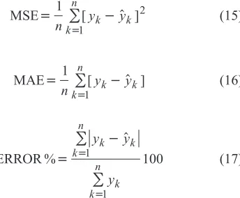
The mean square error (MSE), mean absolute error (MAE), correlation coefficient (R), and error percentage (ERROR%) between the measured and the predicted SSSS and GMD values were used to evaluate the performance of the proposed models. The MSE, MAE, and ERROR% sta-tistics are defined as below:
MSE= å
-=
1 2
1
nk yk yk
n
[ $ ] (15)
MAE= å
-= 1
1
nk yk yk
n
[ $ ] (16)
ERROR %
$ =
-å
å =
=
y y
y
k k
k n
k k
n 1
1
100 (17)
where: $yk denotes the predicted value yk, is the measured value, andnis the total number of observations.
RESULTS AND DISCUSSION
The results on prediction ofSSSSusing MLR and SVM techniques are presented inTable 3. The MAE and MSE values for the MLR model were 0.81 and 0.99, respectively, and an ERROR% value of 12.72% found for this technique. A lower ERROR% value of 2.64% in prediction of SSSS using the SVM model obtained in comparison with the MLR model. The MAE and MSE values for the SVM model were also 0.17 and 0.06, respectively. The coefficient of correla-tion (R) between the measured and predicted SSSS values for the SVM model was 0.98 while it was 0.52 for the MLR model. Therefore, according to the evaluation indices, it appears that there is a more suitability of developing soil shear strength prediction models using SVM approach than traditional regression models. The worse performance of the
MLR model in predicting the measured SSSS values can be also seen in Fig. 1, where the error performance values for the MLR model are more scattered than those for the SVM model. On the other hand, our findings also revealed the significance of combining soil properties with topographic and vegetation attributes together for the estimation of SSSS using the optimized SVM model with SA algorithm.
Table 4 shows the evaluation criterion results for the constructed MLR and SVM models for GMD prediction. The MAE, MSE, R, and ERROR% values for the GMD prediction using the MLR model were 0.08, 0.012, 0.42, and 14.59%, respectively. The SVM model could predict the GMD with more satisfactory performance than the MLR model and a higher correlation coefficient value of 0.97 was obtained for this technique as compared to that obtained by the MLR model. The MAE, MSE, and ERROR% values for GMD prediction using the SVM model were also 0.02, 0.001, and 4.29%, respectively. Higher error values in GMD prediction using the MLR method were also found in comparison with SVM method (Fig. 2).However, a similar trend of error performance values for GMD prediction using both techniques was observed for most of the samples. These results suggest a better performance of SVM techni-que in prediction of the GMD than MLR technitechni-que and thus
Soil property
SVM parameter Kernel
(s)
Intensive (e)
Punishment coefficient (C)
SSSS 0.1 0.09 18
GMD 0.5 0.06 24
T a b l e 2.Optimal values of the SVM parameters resulting from the simulated annealing algorithm analysis for the prediction of the SSSS and GMD properties
Model type
Evaluation criterion
MAE MSE R ERROR %
MLR 0.81 0.99 0.52 12.72
SVM 0.17 0.06 0.98 2.64
T a b l e 3.Goodness-of-fit of proposed MLR and SVM models for the prediction of soil shear strength
Model type
Evaluation criterion
MAE MSE R ERROR %
MLR 0.08 0.012 0.42 14.59
SVM 0.02 0.001 0.97 4.29
the optimized SVM with SA algorithm technique seems to be more reliable in predicting the soil aggregate stability than MLR technique in the site studied.
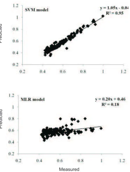
Comparing the obtained results from the proposed MLR and SVM models indicated that the optimized SVM model with SA algorithm was better in predicting the investigated soil properties than the MLR model (Tables 3 and 4). The obtained coefficient of determination (R2) values between the measured and the predicted SSSS and GMD values using both models also confirm this finding (Figs 3 and 4). The R2 value between the measured and the predicted SSSS values using the MLR model was 0.27 while it was 0.95 using the SVM model (Fig. 3). Furthermore, the coefficient of deter-mination values for the GMD prediction using the MLR and SVM models were 0.18 and 0.95, respectively (Fig. 4).
A reason for this finding (better performance of SVM approach in predicting the investigated soil properties) may be attributed to the less data available for developing reasonable MLR models. In contrast, the SVM models could recognize the relationships with relatively less data because
of their distributed and parallel computing nature. A second reason why the linear modeliemultiple regression might be unreliable to predict the SSSS and GMD in the study area is that the effect of the predictors on the dependent variable may not be linear in the nature. In other word, the SVM models could probably predict the SSSS and GMD with more satisfactory performance owing to their more flexi-bility and capaflexi-bility to model non-linear relationships.In fact by using the kernel function in constructing of SVM model, the original inputs are first non-linearly mapped into the feature space, and the resulted å-SVM becomes so fle-xible that it can be used to deal with the complicated non-linear regression problem (Liet al.,2009).Furthermore, the low accuracy of the MLR approach in estimating the mea-sured SSSS and GMD values might be associated with the sample distribution, spatial variation, and the study area scale effects. The major conceptual limitation of all regression techniques that is, one can only ascertain relationships but never be sure about underlying causal mechanism, should be also considered (Yilmaz and Yuksek, 2009).
Fig. 1.Comparison of observed error values in SSSS prediction using SVM and MLR models.
Fig. 2.Comparison of observed error values in GMD prediction using SVM and MLR models.
ERROR
ERROR
Sample number
There are limited published studies dealing with the use of SVMs in soil sciences: Lamorski et al.(2008), for in-stance, estimated soil hydraulic parameters from measured soil properties using SVMs. They reported that 3-parameter SVMs performed generally better than or with the same accu-racy as eleven parameter ANNs. Twarakaviet al.(2009) de-veloped SVM models for estimating the hydraulic para-meters describing the soil water retention and hydraulic con-ductivity. They stated that the SVM-based method predic-ted the hydraulic parameters better than the ANN-based me-thod. Wanget al.(2009) compared different artificial intel-ligence methods for forecasting monthly discharge time se-ries. They concluded that SVM model was able to obtain bet-ter forecasting accuracy in bet-terms of the various evaluation measures during the both training and validation phases.
CONCLUSIONS
1. An optimized support vector machines with the si-mulated annealing algorithm was evaluated for predicting some soil propertiesiesoil shear strength and soil aggre-gate stability and achieved greater estimation accuracy comparable to that of traditional multiple-linear regression.
2. The effects of soil properties, topographic and vege-tation attributes on soil shear strength and soil aggregate sta-bility demonstrated the suitasta-bility of developing prediction functions using SVMs.
3. According to the advantages associated with the use of the SVM over traditional linear regressions, studies on this approach should continue in an effort to relate soil properties to the basic soil characteristics and its advantages should motivate soil scientists to work further on it in the future.
REFERENCES
Azizi N. and Zolfaghari S., 2004.Adaptive temperature control for simulated annealing: a comparative study. Computers Operations Res., 31, 2439-2451.
Burges C.J.C., 1998.A tutorial on support vector machines for pat-tern recognition. Data Mining Knowledge Disc., 2, 121-167. Canasveras J.C., Barron V., Del Campillo M.C., Torrent J., and Gomez J.A., 2010.Estimation of aggregate stability indices in Mediterranean soils by diffuse reflectance spec-troscopy. Geoderma, 158, 78-84.
CantonY., Sole-Benet A., Asensio C., Chamizo S., and Puigde-fabregas J., 2009.Aggregate stability in range sandy loam soils: relationships with runoff and erosion. Catena, 77, 192-199.
Fig. 3.Scatter plots displaying the relationships between measured and predicted values of SSSS using SVM and MLR models.
Measured
Predicted
Predicted
Fig. 4.Scatter plots showing the relationships between measured and predicted values of GMD using SVM and MLR models.
Measured
Predicted
Cristianini N. and Taylor J.S., 2000.An Introduction to Support
Vector Machines and Other Kernel-Based Learning Me-thods. Cambridge University Press, New York, USA. Gee G.W. and Bauder J.W., 1986.Particle size analysis. In:
Methods of Soil Analysis (Ed. A. Klute). ASA Press, Madison, WI, USA.
Geng X., Xu J., Xiao J., and Pan L., 2007.A simple simulated annealing algorithm for the maximum clique problem. Information Sci., 177, 5064-5071.
Huang Y., Lan Y., Thomson S.J., Fang A., Hoffmann W.C., and Lacey R.E., 2010.Development of soft computing and applications in agricultural and biological engineering. Comp. Electr. Agric., 71, 107-127.
Kemper W.D. and Rosenau K., 1986.Size distribution of aggre-gates. In: Methods of Soil Analysis (Ed A. Klute). Am. Soc. Agron., Madison, WI, USA.
Kêsik T., B³a¿ewicz-WoŸniak M., and Wach D., 2010.Influence of conservation tillage in onion production on the soil organic matter content and soil aggregate formation. Int. Agrophys., 24, 267-273.
Kirkpatrick S., Gelatt C.D., and Vecchi M.P., 1983. Optimiza-tion by simulated annealing. J. Sci., 220, 671-680.
Lamorski K., Pachepsky Y., S³awiñski C., and Walczak R.T., 2008. Using support vector machines to develop pedo-transfer functions for water retention of soils in Poland. Soil Sci. Soc. Am. J., 72, 1243-1247.
Li H., Liang Y., and Xu Q., 2009.Support vector machines and its applications in chemistry. Chemometrics Intell. Lab. Sys., 95, 188-198.
Mo Z., Xie H., Liu H., and Li F., 2010.Parameter optimization of
SVM based on HQGA. Proc. 16th Int. Conf. Natural
Computation, August 10-12, Yantai, China.
Nelson D.W. and Sommers L.P., 1986.Total carbon, organic carbon and organic matter. In: Methods of Soil Analysis: (Ed. A.L. Page). ASA Press, Madison, WI, USA.
Nelson R.E., 1982.Carbonate and gypsum. In: Methods of Soil Analysis (Ed. A.L. Page). ASA Press, Madison, WI, USA. Ohu J.O., Mamman E., and Mustapha A.A., 2009.Impact of
organic material incorporation with soil in relation to their shear strength and water properties. Int. Agrophysics, 23, 155-162.
Twarakavi N.K.C., Simunek J., and Schaap M.G., 2009.
Development of pedotransfer functions for estimation of soil hydraulic parameters using support vector machines. Soil Sci. Soc. Am. J., 73, 1443-1452.
van Bavel C.H.M., 1950.Mean-weight diameter of soil aggre-gates as a statistical index of aggregation. Soil Sci. Soc. Am. Proc., 14, 20-23.
van Laarhoven P.J.M. and Aarts E.H., 1988.Simulated anneal-ing: theory and applications. Kluwer Academic Press, Dordrecht, The Netherlands.
Vapnik V., 1995. The Nature of Statistical Learning Theory. Wiley Press, New York, USA.
Wang W.C., Chau K.W., Cheng C.T., and Qiu L., 2009.A compa-rison of performance of several artificial intelligence methods for forecasting monthly discharge time series. J. Hydrol., 374, 294-306.
Yilmaz I. and Yuksek G., 2009.Prediction of the strength and elasticity modulus of gypsum using multiple regression, ANN, and ANFIS models.Int. J. Rock Mechanics Mining Sci., 46, 803-810.