Application of Soft Computing Techniques for Handoff Management in Wireless Cellular Networks

(1)

7 International Journal of Engineering and Management Research, Vol.-2, Issue-6, December 2012

ISSN No.: 2250-0758

Pages: 7-20

www.ijemr.net

Analysis of One Dimensional Beam Problem Using Element Free Galerkin

Method

Vijender1, Sunil Kumar Baghla2

1

M.Tech Student, 2Assistant Professor

Department of Mechanical Engineering, Yadvindra College of Engineering Punjabi University Guru Kashi Campus Talwandi Sabo, Bathinda, Punjab, INDIA

ABSTRACT

For analysis of mechanical parts in designing it needs to calculate mechanical properties of element or a part, for this we start from the stress/strain calculation. Although stress/strain problems can be solved analytically, but for high accuracy, time to solve the problem and for solving the typical problems (e.g. irregular shaped part, beams with various loading conditions, moving boundary problems etc.) process needs a method so that above problems can be solved easily or minimized.FEM is the primary method for simulation of parts. But there is a problem associated with FEM that it is complicated to solve problems of discontinuous stress and strain or distortion or deformed body. Because re meshing problem arises in the procedure. It consumes most of the analysis time. So, there is a procedure to overcome from this problem that is Mesh free Methods. This saves the re meshing time. Because, this method is based on nodes calculation rather than element calculation In this work different mesh free methods are discussed and the mainly EFGM (ELEMENT FREE GALERIKIN METHOD) is used to solve the problem. A problem of varying cross section is solved by this method. The results are compared with the FEM solution as well as with the analytical solution for the validation of results. The main work is to validate the results after that the effect of the weight function, domain of influence etc. are discussed as well as compared their results are compared.

Keywords —_{Element Free Galerkin Method, FEM,}

Mesh free methods, one dimensional stress, varying cross sectional beam.

I. INTRODUCTION

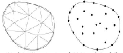
Mesh free methods as the name indicates there are no mesh generation in this method as in case of the FE method. The calculation is based on the nodal parameters. These methods have some advantages over FE method.

Fig 1.1 Discretization of FEM and Mesh free methods

(2)

8

methods, however, a conforming mesh with sufficient quality may be impossible to maintain. Even if it is possible, the remeshing process degrades the accuracy considerably due to the perpetual projection between the meshes, and the post-processing in terms of visualization and time-histories of selected points requires a large effort. The shape functions of MMs may easily be constructed to have any desired order of continuity. MMs readily fulfill the requirement on the continuity arising from the order of the problem under consideration. In contrast, in mesh-based methods the construction of even C1 continuous shape functions needed e.g. for the solution of forth order boundary value problems may pose a serious problem. No post-processing is required in order to determine smooth derivatives of the unknown functions, e.g. smooth strains. Special cases where the continuity of the mesh free shape functions and derivatives is not desirable, e.g. in cases where physically justified discontinuities like cracks, different material properties etc. exist, can be handled with certain techniques. For the same order of consistency numerical experiments suggest that the convergence results of the MMs are often considerably better than the results obtained by mesh-based shape functions. In practice, for a given reasonable accuracy, MMs are often considerably

more time-consuming than their mesh-based

counterparts. Mesh free shape functions are of a more complex nature than the polynomial-like shape functions of mesh-based methods. Number of integration points for a sufficiently accurate evaluation of the integrals of the weak form is considerably larger in MMs than in mesh-based methods. At each integration point the following steps are often necessary to evaluate mesh free shape functions: Neighbour search, solution of small systems of equations and small matrix-matrix and matrix vector operations in order to determine the derivatives. Most MMs lack Kronecker delta

property, i.e. the mesh free shape functions Φi do not

fulfill Φ_i(xj) = δij . This is in contrast to mesh-based

methods which often have this property. The imposition of essential boundary conditions requires certain attention in MMs and may degrade the convergence of the method.

II. LITERATURE REVIEW

III.

Belytschko et. al [1] used the moving least-squares interpolants to construct the trial and test functions for the variational principle (weak form) and weight functions. In contradistinction to DEM, they introduced certain key differences in the implementation to improve the accuracy. Also in

their paper, they illustrated these modifications with the examples where no volumetric locking occurs and the rate of convergence highly exceeded that of finite

elements. Chen et. al [2] Domain integration by

Gauss quadrature in the EFGM adds considerable complexity to solution procedures. A strain smoothing stabilization for nodal integration is proposed to eliminate spatial instability in nodal

integration. For convergence, an integration

constraint (IC) is introduced as a necessary condition for a linear exactness in EFGM. The gradient matrix of strain smoothing is shown to satisfy IC using a divergence theorem. No numerical control parameter is involved in the proposed strain smoothing stabilization. The numerical results show that the accuracy and convergent rates in the mesh-free method with a direct nodal integration are improved considerably by the proposed stabilized conforming nodal integration method. It is also demonstrated that the Gauss integration method fails to meet IC in mesh-free discretization. For this reason the proposed method provides even better accuracy than Gauss integration for EFGM as presented in several numerical examples. In a paper a new body integration technique is presented and applied to the evaluation of the stiffness matrix and the body load

vector of elastostatic problems obtained by Duflot

and Dang [3] in mesh less method. It does not work on a partition of the integration domain into small cells, but rather on a partition of unity by a set of moving least squares shape functions each defined on a small patch that belongs to a set of overlapping patches covering the domain and so leads to a truly mesh less method and gives results that this method is especially useful when the nodes are irregularly

scattered. Soparat et. al [4] has extended the EFGM

to include nonlinear behavior of cracks in 2D concrete. A cohesive curved crack is modeled by

using several straight-line interface elements

connected to form the crack. The constitutive law of the crack is considered through the use of these interface elements. The stiffness equation of the domain is constructed by directly including, in the weak form of the system equation, a term related to the energy dissipation along the interface elements. Using the interface elements in conjunction with the EFG method allows crack propagation to be traced easily and without any constraint on its direction. The proposed method is found to be an efficient method

for simulating propagation of cracks in concrete. Gu

et. al [5] discussed that EFGM is computationally

expensive for many problems. A coupled

(3)

9

preserved on the interface of the two domains where the EFG and BE methods are applied. The present coupled EFG/BE method has been coded in FORTRAN. The validity and efficiency of the EFG/BE method are demonstrated. It is found that the present method can take the full advantages of both EFG and BE methods. It is very easy to implement, and very flexible for computing displacements and stresses of desired accuracy in

solids with or without infinite domains. Rabczuk et.

al [6] presented an in-depth presentation and survey of mesh-free particle methods. Several particle approximation are reviewed; the SPH method, corrected gradient methods and the Moving least squares (MLS) approximation. The discrete equations are derived from a collocation scheme or as Galerkin method. Special attention is paid to the treatment of essential boundary conditions. A brief review over radial basis functions is given because they play a significant role in mesh-free methods. Finally, different approaches for modeling discontinuities in

mesh-free methods are described. Zhang et. al [7]

used moving least-square technique to construct shape function in the Element Free Galerkin Method at present, but sometimes the algebra equations system obtained from the moving least-square approximation is ill-conditioned and the shape function needs large quantity of inverse operation. The weighted orthogonal functions are used as basis ones, the application in the calculation of plate bending shows that the improved moving least-square approximation is effective and efficient.

IV. METHODOLOGY

In the methodology two case studies are being discussed with their analytical, FEM and EFGM solution methodology. The case studies are stated following:

3.1 Case Study 1

In this problem a regular cross section beam is selected. The beam is loaded with axial concentrated load. The problem is given as:

A steel rod of length 1m is subjected to an axial load of 5KN and area of cross section is 250mm. take E=2*10^5 N/mm2. [9] Now we will find the solution by analytical, FEM and EFGM.

L=1M

P=5kN

Fig.4.1 steel bar

Where P is the concentrated load and L is the length of the steel bar.

Calculate:

1. Displacement

2. Stress at different points of the bar.

Analytical Solution

The bar is discritized in the four equal parts, to calculate the required result at different nodal points. Because there are 5 nodal points so there will be five results of displacements as well as for the stress.

The calculation for the analytical results starts from the Hooke’s law

(3.1) Where is stress,

(3.2)

E is the modulas of elasticity of the steel bar;

is strain in the material.

(3.3)

u is Displacement,

(3.4)

Now from the above given equations analytical results can be found easily at different nodes. Equation 3.2 gives the stress at five nodes of the steel bar and equation3.4 gives the displacement at the consecutive nodal points.

The calculated results of the analytical solution are in the next chapter results and discussion. These results are the landmark for further work, because these results are compared with the FEM results later on with the EFGM results.

FEM results

The bar is divided in four equal elements (250mm) and the area of each element is regular throughout the bar. After that a separate stiffness matrix is generated for each element using the formula

(3.5)

So K1; K2; K3; K4 are generated using the

given values of area (A), modulas of elasticity (E) and length of element (L). These values are getting

together in a stiffness matrix K.

(4)

10

And the stiffness equation is generated

KU=P (3.6)

Where U is displacement vector given as;

U= (3.7)

And P is force vector given as;

P= (3.8)

U=K-1P (3.9)

(3.9) Using the equation3.5 the stiffness matrix for

each element is generated. Now generated stiffness matrix is assembled into one stiffness matrix K. The equation3.8 is load vector in this the given concentrated load is being put here P5 is 5kN because load is at extreme point and other nodes are not loaded. Now the result is calculated using the equation3.9. This will give the displacement of each element.

(3.10)

(3.11)

Equation3.10 gives stress at first points. Like this equation3.11 gives the stress at second point

and so on the stress is calculated up to . The

results calculated by above equations are compared with analytical results. Now next step is to calculate the results with the help of EFGM.

The second problem is selected a varying cross sectional beam whose area is decreasing from fixed end to free end. The load is again concentrated at the free end.

The equation for stress analysis is shown in equation 1 [10]. It is simple stress problem and given

as. Consider an linear elastic bar [10] of length L=1m

with a varying cross section A(x), where Ar(x),E(x)

Fig.3.2 Elastic bar of varying cross section

; [19] (3.12)

A0= 0.01 m2; (3.13)

Young's modulus ;

The bar is rigidly supported at the left end and at the

right a concentrated force P is applied;

P= 10000N Calculate:

1. Displacement

2. Stress at different points of the bar.

Analytical results

They can be calculated using the

equation3.1, 3.2 and 3.3. For the varying cross section the equations for the displacement and stress becomes as under

Displacement,

[10] (3.14)

And stress as,

[10] (3.15)

The beam is discritized in three equal elements. The displacement and stress at consecutive nodes is calculated analytically using the equations 3.14 and 3.15

FEM results

The bar is divided in three equal elements of .33333 m and the area of each element is calculated at the center of the element so that three parts can be made of equal cross section.

After that a separate stiffness matrix is generated for each element using the formula

(3.16)

So K1; K2; K3 are generated using the given

values of area (A(x)), modulas of elasticity (E) and length of element (L). These values are getting

together in a stiffness matrix K.

And the stiffness equation is generated

KU=P (3.17)

Where U is displacement vector given as;

10000

N

x

X

=

X

(5)

11

U= (3.18)

And P is force vector given as;

P= (3.19)

(3.19)

U=K-1P (3.20) (3.20) The equation 3.20 gives the displacement of

the each element. Now stress is calculated as below

B= [1 -1] (3.21)

(3.22) The equation 3.22 gives the stress at three nodes putting the corresponding values. The results are compared with the analytical solution.

3.3 EFGM solution

Consider a bar whose cross sectional area is Ar(x) and its length is L. Now assume that any force is applied in the direction of extension of body or in the longitudinal axis (x-axis). That force is point load P [N] and distributed load b(x) [N/m]. The body is in only tensile loading no shear force or bending loads will be considered. Only stretching in its direction resulting increase in its length. E(x) is the Young’s modulus of elasticity of the material. Now there will be displacement in the bar due to applied loads that is u(x) that will be in one direction so we can say it is the One Dimensional elastic problem. The problem

will involve displacement u(x), stress σ(x) and strain

ε(x). This can be calculated by applying boundary

conditions. Now refer the fig3.2 and Consider a small

elementary strip of length ∆x

Fig.3.4 small element of bar

By equilibrium law force can be written as

P(x+∆x)-P(x)+b(x)=0 (3.23)

By Taylor’sformula,

(3.24)

We know that,

P(x) =σ(x)Ar(x) (3.25) And by hook’s law,

σ(x)=E(x)ε(x) (3.26) so equation (1) can be written as,

(3.27)

And further more equation becomes,

(3.28) Strain in the strip,

(3.29)

So,The strong form is given as,

(3.30)

The equation 3.30 gives the strong form for the elastic problems of cantilever when it is loaded with point load axially at free end. So this equation is for both case studies.

3.3.1 Moving Least Squares

It is the starting point of the Element Free

Galerkin Method. For the approximation of u(x)

which is a domain Ω by

u(x)= =pT(x)a(x) , (3.31)

j=1,2,…,m

where p1(x)=1 and pj(x)aremonomial basis

in the space coordinates xT=[x, y] and is known and

complete basis, A linear and quadratic basis in one

dimension can be given by

pT(x)=[1,x], m=2 (3.32)

pT(x)=[1,x,x2], m=3 (3.33)

and linear and quadratic for two dimensions can be

given as

pT(x)=[1,x,y], m=3 (3.34)

pT(x)=[1,x,y,x2,xy,y2], m=6 (3.35)

The aj(x) is unknown coefficients, which is

solved by moving least squares procedure using

nodal points, a(x) is obtained at x by minimizing a

weighted discrete Least-Squares norm J as

(3.36)

P(x+

∆

x)

b(x)

∆

x

(6)

12

here n is the number of points in the neighborhood of

x for which the weight function w(x-xi)≠0 and uiis the

nodal value of u at x= xi. and this neighborhood of x

is called domain of influence of x (or domain of

influence of node i). The relation between a(x) and u

can be written in the linear equation which is:

A(x)a(x)=B(x)u (3.37)

Or equation can be molded as

a(x)=A-1(x)B(x)u (3.38)

here m is the number of EFG nodes and

these nodes include the domain of influence x. now

A(x) and B(x) are in matrix form and defined as

A(x)= ∑wti(x)p T

(xi)p(xi) (3.39)

Where i=1 to n andwti=w(x- xi),

B(x)=[ w(x- x1) p(x1), ….., w(x- xn) p(xn)]

or

B(x)=[ wt1 p(x1), wt2 p(x2),……….., wtn p(xn)]

(3.40)

So the equation (1) becomes

u(x)= ∑ Φi(x)ui (3.41) (where i=1 to n)

Now MLS shape function Φi(x) can be defined as

Φi(x)= ∑ pj(x) (A-1(x)B(x))ji (3.42)

The continuity of the shape function is Φi(x) is

defined by the continuity of basis function pj;

depends on the smoothness of the matrices A-1(x) and

B(x) and choice of the weight function. The partial

derivativeofΦi(x) can be calculated as

(3.43)

3.3.2 Weight Functions

The weight function (wt(x)=w(x- xi )) plays

an important role in the EFGM’s performance. It

should be selected so that a unique solution a(x) can

be generated. Its value should decrease in magnitude

as the distance increases from x to xi. Now dmxis the

support size for the weight function, dis=sign(x-xi),

and d=dis/dmx. The most commonly used weight

functions are given as:

The cubic and quadratic spline weight

function is more favorable because they provide

continuity and less computationally less demanding.

The singular weight function allows the direct

imposition of essential boundary conditions. So in the

case of singular weight function there is no need of

Lagrange multipliers.

Singular:

(3.44)

Cubic spline

(3.45)

Quadratic spline:

(3.46)

3.3.3 EFGM weak formulation

And the weak formulation is

(3.47) Integrating by parts to above equation Where the natural boundary is condition and is the domain boundary

(7)

13

(3.49)

Rearranging equation,we get

(3.50) The above equation can be written as in the following

form,

[K]{U}={f } (3.51)

Where the matrices [K] and {f} given by

(3.52)

(3.53)

(3.54)

(3.55)

(3.56)

IV. RESULTS AND DISCUSSION

Using the methodology discussed the results are calculated for the case study 1. The calculated results for the case study 1 are;

Using the formula for displacement and stress given in the methodology chapter the analytical results are obtained. Which is shown in Table4.1 the Table4.1

shows the results of case study 1. The column 2nd

shows the displacement in beam at different nodes

displacement is in mm and similarly the 3rd column

shows the stress in the beam at consecutive nodes the

stress is in N/mm2. The result seems continuous.

Table 4.1 Analytical results

Node U Σ

1 0 0

2 0.025 20

3 0.05 20

4 0.075 20

5 0.1 20

FEM Results

For the FEM results the equations given in the methodology section is used. The displacement at different nodes and stress at corresponding nodes are calculated by those equations. Table 4.2 shows the results of FEM

Table 4.2 FEM results

Node U σ (N/mm2)

1 0 0

2 0.025 20

3 0.05 20

4 0.075 20

5 0.1 20

EFGM Results

(8)

14

Table 4.3 EFGM results

Node u σ

1 ₀ ₀

2 _0.0251 _20.0742

3 _0.05 _19.9258

4 _0.0749 _19.9258

5 _0.1 _20.0742

Validation for case study 1

Now analytical, FEM & EFGM results have been calculated according to the methodology. These results are compared for the validation of the EFGM method whether the results are liked to analytical and FEM results or not.

Fig 4.1 Comparison b/w Analytical, FEM and EFGM displacement

The Fig4.2 shows the comparison between analytical, FEM, EFGM results. These results are of only displacement results of three methods at different nodes of the beam. By the comparison a person can see that the EFGM results obtained are continuous and regular as in case of analytical and FEM.

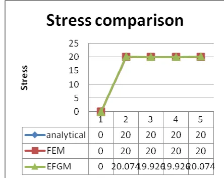
After comparing the displacement results now the stress results of EFGM are compared with the analytical, FEM results the following figure shows the comparison between three methods.

Fig 4.2 Comparison b/w Analytical, FEM and EFGM stress

These results shows that the result obtained in the EFGM method are continuous in case of displacement as well as in case of stress also. The results are accurate and equal to other methods. So this method satisfies the one dimensional elastic problem.

Using the methodology discussed the results are calculated for the case study 1. The calculated results for the case study 1 are;

Using the formula for displacement and stress given in the methodology chapter the analytical results are obtained. Which is shown in Table4.1 the Table4.1 shows the results of case study 1. The

column 2nd shows the displacement in beam at

different nodes displacement is in mm and similarly

the 3rd column shows the stress in the beam at

consecutive nodes the stress is in N/mm2. The result

seems continuous.

Table 4.4 Analytical results

NODE Area u*(1*10^-5) σ*(10^7)

1 .0095 0 0

(9)

15

3 .0056 0.5 0.1785

4 .0034 1 0.2777

FEM Results

For the FEM results the equations given in the methodology section is used. The displacement at different nodes and stress at corresponding nodes are calculated by those equations.

Table 4.5 FEM resul

EFGM Results

For this a MATLAB programme is generated using the EFGM weak formulation results. Like the FEM the stiffness matrix is generated but in this weight function, shape function is added in the stiffness matrix. After that the Lagrange multiplier is used in the boundary conditions. The equation becomes in the form of KU=P. The results are of nodes. These are the discretized equations of the EFGM

Table 4.6 EFGM results

Node Area

u*(1*10^-5) σ

1 0.0095 0 0

2 0.0084 0.1589 0.06658

3 0.0056 0.5293 0.19529

4 0.0034 0.9528 0.32399

Validation for case study 2

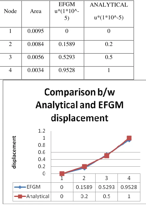
For the validation the results are compared firstly with analytical results. This shows results are favorable; continuous; consistent and like. A combined table for the displacement is made for the comparison. The displacement of the EFGM and Analytical solution is same. We can see the results in Table 4.7 at each node the displacement values are approximately same with negligible differences.

Table 4.7 Comparison b/w Analytical and EFGM displacement

Fig. 4.3 Comparison b/w Analytical and EFGM displacement

The Fig. 4.3 comparing the results of analytical and EFGM lines are overlaping with minor

diffrences. Displacement variation at each node is plotted for both of the methods. In Table 4.8 and Fig. 4.4 the comparisn between FEM and EFGM

Node Area

u*(1*10^-5) σ*(10^7)

1 0.0095 0 0

2 0.0084 0.1983 0.119

3 0.0056 0.4946 0.1778

4 0.0034 0.9844 0.2939

Node Area

EFGM

u*(1*10^-5)

ANALYTICAL

u*(1*10^-5)

1 0.0095 0 0

2 0.0084 0.1589 0.2

3 0.0056 0.5293 0.5

(10)

16

shown these results are also favourable and like results.

Table 4.8 Comparison b/w EFGM and FEM displacement

Node Area

EFGM

u*(1*10^-5)

FEM

u*(1*10^-5)

1 0.0095 0 0

2 0.0084 0.1589 0.1983

3 0.0056 0.5293 0.4946

4 0.0034 0.9528 0.9844

Fig. 4.4 Comparison b/w EFGM and FEM displacement

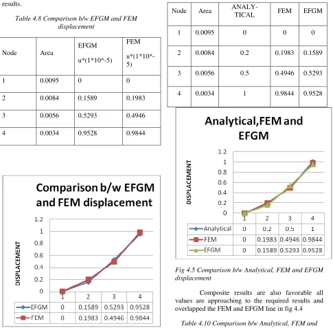
Now the composite results for three methods are generated to check their difference. So a displacement and stress table is generated below;

Table 4.9 Comparison between Analytical, FEM and EFGM displacement

Fig 4.5 Comparison b/w Analytical, FEM and EFGM displacement

Composite results are also favorable all values are approaching to the required results and overlapped the FEM and EFGM line in fig 4.4

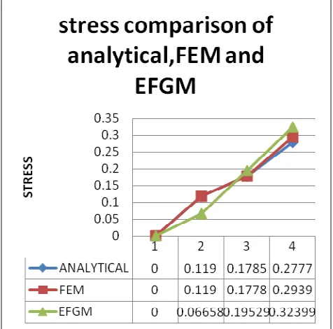
Table 4.10 Comparison b/w Analytical, FEM and EFGM STRESS

Node Area

ANALY-TICAL FEM EFGM

1 0.0095 0 0 0

2 0.0084 0.2 0.1983 0.1589

3 0.0056 0.5 0.4946 0.5293

(11)

17

Fig. 4.6 Comparison b/w FEM and EFGM STRESS

In the case of stress at node 2 it is different

but all other are showing good results for EFGM. Fig. 4.7 Comparison b/w Analytical, FEM and

EFGM STRESS

In Table 4.11 comparison for the stress have been done successfully. The results are positive for the EFGM. Here I can say the results are positive so the method i choose is valid for the selected problem .further the results may be verified. Results like domain of influence if changed effect in the results or change in weight function gives same results or results get changed due to the weight function. So for that following attempt have been done

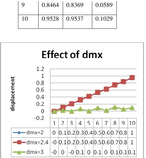
4.3 Effect of dmx on the result

Table 4.12 Effect of dmx on displacement

Node dmx=2 dmx=2.4 dmx=3

1 0 -0.0002

-0.0026

2 0.1064 0.1125 0.0261

3 0.2115 0.2071 -0.002

4 0.3177 0.3209 0.0647

5 0.4235 0.4214 0.0057

6 0.5293 0.5323 0.0962

7 0.6351 0.6309 0.0207

8 0.7413 0.749 0.1154

Node Area

ANALY-TICAL

σ*(10^7)

FEM

σ*(10^7)

EFGM

σ*(10^7)

1 0.0095 0 0 0

2 0.0084 0.119 0.119 0.06658

3 0.0056 0.1785 0.1778 0.19529

(12)

18

9 0.8464 0.8369 0.0589

10 0.9528 0.9537 0.1029

Fig. 4.8 Effect of dmx on displacement

Fig. 4.9 Effect of dmx on stress

Now by the observation of fig 4.7 it is clear that the results are same if the dmx is changed 2 to 2.4 but if it increased further the results get distorted. So for this problem the dmx 2 or 2.4 is best selected domain of influence. Although the displacement gets changed a lot but in fig 4.8 one can see the results of stresses do not change drastically. It changes little bit to the previous results.

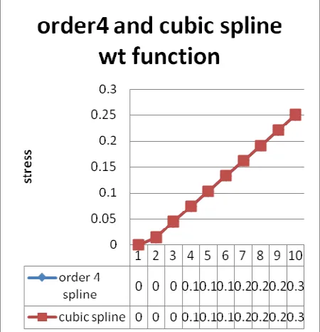
4.4 Effect of Weight Functions on results

Fig. 4.10 Effect of weight function on displacement

Now the change in the weight function is attempted to see the effect of weight function which one is better for this problem. But after the comparison in fig 4.9 it is observed that the result are as continuous and same as they were so there is not any drastic change in the displacement results due to the weight function.

There is not a big change due to the quadric spline weight function from the results of cubic spline. In the fig 4.10 stress results are as they were even at some points they are with same results. So we can say for this type of problem both the weight functions can hold good command over the results.

(13)

19

Fig. 4.11 Effect of weight function on stress

V. CONCLUSION

EFG method is an achievement in the improvement of mesh free methods. In this thysis a MATLAB program has been developed to analyze plane stress problem by EFG method. The obtained results are compared with analytical and FEM results.

In this study, the varying cross section problem has been solved. In this the cantilever beam is subjected to the simply point load at the free end. The applied load is tensile in nature which results in extension or displacement of the bar.

The results obtain in the form of displacement are equal to the FEM as well as to the analytical method. Same in case of stress. So we can say EFGM as a better alternate for the problems.

Change in weight function in programme even does not alter the results the results are same with same continuity. Second change in domain of influence effect the result when it changed to value 3. But between 2-2.7 it holds good results for the problem .The problem is solved by varying the number of nodes which gives the continuity of the results. The results show that EFG method gives the satisfactory results. Which can be seen in any case applied to it. It has been observed that EFG gives accurate results when compared to FEM. Although it is not perfectly mesh less because we need back mesh for integration but re meshing problem is obsolete here as in case of FEM. The time consumed in the EFGM is more as in case of FEM. But the total time

for solution is less because not only cost the most of the time is consumed in the mesh generation. So, the EFG method can be better alternate to analyze structure problems. If the better no of nodes and quadrature points are selected the best results can be achieved.

VI. FUTURE SCOPE

The extension of EFG to bending problems such as beams of varying cross section loaded with self-weight or uniformly distributed load can be done by this generated code. For more work different material models such as laminated composites, and nonlinear problems, temperature stresses problem on these types of problems can be analyzed. More over this dynamic problem on this can be done .the problem here analyzed can be extended to 2D and 3D work to check the results whether it holds same relation or not. One more topic we can add to future work is temperature stresses on this type of problems and temperature distribution in with conduction, convection or radiation. So for this topic there is a vast area to work one can say it’s the infancy period of this field so it need more work to do.