RESEARCH NOTE
EFFECTS OF DIRECTIONAL SUBDIVIDING ON ADAPTIVE
GRID-EMBEDDING
M. Ameri
Department of Mechanical Engineering, University of Shahid Bahounar Kerman, Iran, [email protected]
E. Shirani
Department of Mechanical Engineering, Isfahan University of Technology Isfahan, Iran, [email protected]
(Received: January 5, 2002 – Accepted in Revised Form: December 12, 2002)
Abstract The effects of using both directions and directional subdividing on adaptive grid-embedding on the computational time and the number of grid points required for the same accuracy are considered. Directional subdividing is used from the beginning of the adaptation procedure without any restriction. To avoid the complication of unstructured grid, the semi-structured grid was used. It is used to solve three test cases, transonic and supersonic inviscid flows in channels with circular arc bump and with convergent part. The Euler equations are integrated to steady state by an explicit, finite volume, Ni’s Lax-Wendroff type. In this work, multi-grid technique is applied to increase the convergence rate. The directional subdividing is more complex than both directions subdividing. However, the results show that for the same accuracy, directional subdividing considerably reduces the number of grid points and the computational time.
Key Words Directional subdividing, Embedding, Adaptive, Grid Generation, Euler equations
ﻩﺪﻴـﮑﭼ
ﻩﺪﻴـﮑﭼ
ﻩﺪﻴـﮑﭼ
ﻩﺪﻴـﮑﭼ
ﺩﺍﺪﻌﺗﻭﻪﺒﺳﺎﺤﻣﻥﺎﻣﺯﺮﺑﻲﺘﻬﺟﺕﺭﻮﺻﻪﺑﻭﺖﻬﺟﻭﺩﺭﺩﻝﻮﻠـﺳﻢﻴـﺴﻘﺗﺮـﺛﺍ ﻱﺎﻫﻩﺮﮔ
ﺵﻭﺭﺭﺩﻪﮑﺒﺷ
ﺖﺳﺍﻪﺘﻓﺮﮔﺭﺍﺮﻗﻲﺳﺭﺮﺑﺩﺭﻮﻣﻩﺪـﺷﻩﺩﺍﺩﺎـﺟﻪﮑﺒـﺷﻖﻴـﺒﻄﺗ
. ﻪﻠﺣﺮﻣﻦﻴﻟﻭﺍﺯﺍﻲﺘﻳﺩﻭﺪﺤﻣﭻﻴﻫﻥﻭﺪﺑﻲﺘﻬﺟﻢﻴﺴﻘﺗ
ﺖﺳﺍﻩﺪـﺷﻪﺘـﻓﺮﮔﺭﺎـﮑﺑﻖﻴـﺒﻄﺗ
.
ﺒﺷﺯﺍ،ﻥﺎﻣﺯﺎﺳﻲﺑﻪﮑﺒﺷﻱﺎﻫﻲﮔﺪﻴﭽﻴﭘﺯﺍﺰﻴﻫﺮﭘﻱﺍﺮﺑ ﻩﺩﺎﻔﺘﺳﺍﻪﺘﻓﺎﻳﻥﺎﻣﺯﺎﺳﻪﻤﻴﻧﻪﮑ
ﺖـﺳﺍﻩﺪـﺷ
. ﺭﺩﻲﺗﻮﺻﺍﺮﻓﻭﻲﺗﻮﺻﺍﺮﺗﺝﺰﻟﺮﻴﻏﻥﺎﻳﺮﺟﺭﺩﻝﺪﻣﻪﻠﺌﺴﻣﻪﺳﻲﺘﻬﺟﻢﻴـﺴﻘﺗﺮـﺛﺍﻲـﺳﺭﺮﺑﺭﻮﻈﻨـﻣﻪـﺑ
ﺖﺳﺍﻩﺪﺷﻞﺣﺍﺮﮕﻤﻫﺖﻤﺴﻗﮏﻳﻭﻱﻭﺮﻳﺍﺩﻱﺎﻨﺤﻧﺍﺎﺑﻱﺎﻫﻝﺎﻧﺎﮐ
. ﻢﺠﺣﺢﻳﺮﺻﺵﻭﺭﮏﻳﻂﺳﻮﺗﺮﻠﻳﻭﺍﺕﻻﺩﺎﻌﻣ
ﺲـﮐﻻﺵﻭﺭﺱﺎـﺳﺍﺮـﺑﻲـﻟﺮﺘﻨﮐ
ﻉﺍﺪﺑﺍﻲﻧﻂﺳﻮﺗﻪـﮐﻑﻭﺭﺪـﻧﻭ
ﺖﺳﺍﻩﺪﻳﺩﺮﮔﻞﺣ،ﻩﺪﺷ
. ﺪﻨﭼﺵﻭﺭﻦﻴﻨﭽﻤﻫ
ﺖﺳﺍﻪﺘﻓﺮﮔﺭﺍﺮﻗﻩﺩﺎﻔﺘﺳﺍﺩﺭﻮﻣﻲـﻳﺍﺮﮕﻤﻫﺕﺪـﺷﺶﻳﺍﺰـﻓﺍﻱﺍﺮـﺑﻱﺍﻪﮑﺒـﺷ
. ﺯﺍﺮﺗﻩﺪﻴﭽﻴﭘﺭﺎﻴﺴﺑﻲﺘﻬﺟﺪﻨﭼﻢﻴﺴﻘﺗ
ﺪﺷﺎﺑﻲﻣﺖﻬﺟﻭﺩﺮﻫﺭﺩﻢﻴﺴﻘﺗ
. ﻱﺍﻪﻈﺣﻼﻣﻞﺑﺎﻗﺭﻮﻃﻪﺑﻲﺘﻬﺟﻢﻴﺴﻘﺗﻥﺎﺴﮑﻳﺖﻗﺩﺎﺑﻪﮐﺪﻨﻫﺩﻲﻣﻥﺎﺸﻧﺞﻳﺎﺘﻧﺎﻣﺍ
ﻭﻪﮑﺒﺷﻡﺯﻻﻱﺎﻫﻩﺮﮔﺩﺍﺪﻌﺗ ﺪﻫﺩﻲﻣﺶﻫﺎﮐﺍﺭﻪﺒﺳﺎﺤﻣﻥﺎﻣﺯ
.
1. INTRODUCTION
In traditional methods, numerical solution of Euler and Navier-Stoks equations are carried out in a fixed grid. For most practical problems, flow fields contain several length scales due to the presence of shock waves, boundary and shear layers, regions of leading and trailing edges, etc. The order of magnitude of such dominant length scales is smaller than the main flow length scales. For intelligent use of computational sources, grid is
The use of embedding adaptive grid has been center of attention by many researchers recently. In such techniques, the cells are locally divided in the regions of large errors or flow property gradients. Indeed, the nodes are added in these regions. Hence, the equations are solved in a composite grid, a fixed global grid and adaptively embedded patches in the special regions. The simplest and easiest way of dividing the grid cells is to divide each cell into four cells. This technique has been used in vast verity of problems [1-6].
The subdividing a quadrilateral by quadsection increases the number of cells. Some of these cells are unnecessary and inefficient. To avoid such unwanted cells, directional adaptation is used. In this technique, locally refined cells are introduced only in the direction of the flow property gradients. Kallinderis and Baron [7] used directional adaptation techniques for various compressible laminar flows. They used the directional adaptation only in the final stage of the adaptation. Davis and Dannenhofer [8] used adaptive grid-embedding technique to simulate 3-D inviscid flows. They applied directional subdivision technique on block-structured inputs, the so-called chunks. Although this method makes the algorithm simple, but it creates extra cells and most of the cells are divided into four cells. This paper deals with the technique that uses directional adaptation from the very beginning of the adaptation procedure and throughout the flow field. It is shown that this technique produces the minimum number of grid points and therefore it is more efficient algorithm compare to the techniques that are used by others.
2. GOVERNING EQUATIONS AND NUMERICAL METHOD
The invisid compressible fluid flow is governed by the Euler equations. They represent conservation of mass, momentum and energy. For unsteady two-dimensional flows: ∂ ∂ + ∂ ∂ − = ∂ ∂ y G x F t
U (1)
where ρ + ρ ρ ρ = ρ ρ + ρ ρ = ρ ρ ρ = 0 2 0 2 vh P v uv v G uh uv P u u F e v u U (2)
and for perfect gases
(
2 2)
0 e p 1P 21 u v
h + +
ρ − γ γ = ρ +
= (3)
where ρ, u and v, e, p, h0 and γ are density, velocity
components in the x and y directions, total energy per unit volume, static pressure, total enthalpy and specific heat ratio respectively.
The unsteady Euler equations are integrated to steady state by an explicit, finite volume, Lax-Wendroff type time-marching that was developed by Ni [9]. Local time steps are used to accelerate convergence to steady state solution. In addition, Ni’s multiple-grid acceleration technique is also used to couple the solution on various embedded grids and to accelerate overall convergence rate.
3. ADAPTIVE GRID-EMBEDDING METHOD
As mentioned earlier, in grid-embedding methods, the cells are locally divided in the regions of large error or gradient. To do this, the algorithm must sense large gradient or error regions and automatically divide the cells in these regions. The process is repeated several times and therefore local embedded grids become finer and finer in order to resolve special regions adequately.
[7,8]. In this work, directional subdividing is used from the beginning of the adaptation procedure and throughout the flow field without any restriction.
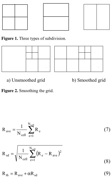
In order to avoid large changes in the grid size, which introduces additional computational errors, local smoothing of the grid-embedding levels is performed. This ensures that only one subdivision difference arises at the interfaces (Figure 2). In addition, the islands and holes must be removed. The cells that the two opposite sides of their neighbors have been divided, are called holes and the divided cells that non of their neighbors has been divided, are called islands.
Adaptation Strategy
One of the basic steps in the embedding adaptive technique is to set adoption parameter and threshold to detect the existence and track the evaluation of special features of the flow fields such as shock waves. The first difference of density is the criterion used in this paper to calculate the adoption parameter. The procedure is as follows:1. If the quadsection is used, the maximum number of absolute values of density differences in each cell is calculated and is chosen as the adaptation parameter.
(
2 1, 3 2, 4 3, 1 4)
maxR= ρ −ρ ρ −ρ ρ −ρ ρ −ρ (4)
where, 1, 2, 3, and 4 indicate the nodes surrounding each cell.
If the bisection (directional subdividing) is used, the absolute values of the density differences of the two opposite walls will be used as the adaptation parameter.
4 1 3 2 1
R
=
ρ
+
ρ
−
ρ
−
ρ
(5)1 2 4 3 2
R = ρ +ρ −ρ −ρ (6)
2. The average, Rave, and standard deviation, Rsd, are used to calculate the threshold, Rth [8].
∑
=
= cell
N
1 e
e cell
ave N1 R
R (7)
(
)
∑
=
−
= cell
N
1 e
2 ave e cell
sd N1 R R
R
(8)
sd ave
th R R
R = +α (9)
The threshold is compared with the adoption parameter in each cell and if adoption parameter is bigger, then the cell will be divided. The value of the parameter αis chosen empirically. Too Large or too small values of αmay cause deficient or extra cells to be refined respectively. It is usually chosen between 0.3 and 0.8 and in this work, it is found that 0.6 is suitable.
Data Structure
Hierarchical quadtree grid generation offers an efficient method for the spatial discretization of arbitrary shaped two-dimensional domains. It consists of recursive algebraic splitting of sub-domains into quadrants, leading to an ordered hierarchical data structure with regard to the storage of mesh information [10,11]. The hierarchical quadtree grids are ideally suited to multiple-grid.With some modifications to the quadtree structure, the approach proves highly flexible and Figure 1. Three types of subdivision.
a) Unsmoothed grid b) Smoothed grid
has been adopted for the adaptive grid-embedding procedure. The quadtree method is based on family branches and their neighbors. Thus, the new generations (children) and the parent of each cell are known. If directionally subdividing is not used, the cells that are divided at the same level will be identified as neighbor for each cell. For example, the cell D in Figure 3-a has the neighbor E in its right and has no neighbor on its left. However, the neighbor on the right side of cell A is B. If the directional subdividing is used, several different cases will occur. There may be cells that are divided at the same level, but the newborn divided cells have no neighbor in one side, or the neighbor is in different level. Figure 3-b shows this matter clearly. In this figure, there is no neighbor in the left side of cell E. However, the neighbor on the left side of the cell B is D. In this data structure, the nodes corresponding to each cell must be specified and in the directionally subdividing, types of subdivision for parent cells must be known.
Interface Nodes
A consequence of gridembedding is the internal boundaries between cells with different levels. An interface is distinguished by an abrupt change in the cell size. The grid lines
A
D
C E
F
B C D
A
E F
G B H
a) both directions subdivision b) directional subdivision
Figure 3. Defining neighbors.
Figure 4. Elimination of interface nodes by employing triangular and quadrilateral cells.
0 0.5 1 1.5 2 2.5 3
0 0.5 1
0 0.5 1 1.5 2 2.5 3
0 0.5 1
0 0.5 1 1.5 2 2.5 3
0 0.5 1
0 0.5 1 1.5 2 2.5 3
0 0.5 1
0 0.5 1 1.5 2 2.5 3
0 0.5 1
0 0.5 1 1.5 2 2.5 3
0 0.5 1
may be continued across the interface or cut off by the interface. In the latter, cells contain extra node at the midside, called hanging nodes. In this paper, the hanging nodes are removed by transition of local connections to surrounding nodes such that triangular and quadrilateral cells are produced (Figure 4). This method is simple and conservative.
4. RESULTS
Three model problems are considered to evaluate the accuracy and efficiency of the technique. They are transonic and supersonic flows on a channel with circular arc wall and supersonic flow in a converging nozzle. In all cases, when the convergence criterion,δ
( )
ρv max, is reached 10−5,the adaptation is done. The final convergence criterion has also been chosen to be smaller than10−5.
Transonic Flow in a Channel with Circular
Arc
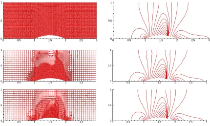
The first case is transonic flow in a channel with a circular arc bump with inlet Mach number of 0.675. The height of the channel is equal to thelength of the bump and the maximum height of the bump is %10 of inlet height. The initial grid is 49
×
17 and the embedding procedure is applied twice. Figure 5 shows the generated grids and the Mach number contours for three different grid configurations. They are uniform fine grid, embedded grid without directional embedding and with directional embedding. In order to get the same accuracy, especially in the areas, which high flow gradient exists, the size of each cell in the fine grid configuration is set to be the same as the smallest size in adapted grid case. The number of grid points for the fine grid configuration is 12545, for the embedded without directional embedding is 3541, and for the directional embedding this number is reduced to 2272. The results of adaptive grid cases show that the same accuracy, compared to the results for fine grid, is obtained with regard to the location and thickness of the shock waves and general flow patterns. When the directional embedding is used, fewer wiggles are seen in the results compared to the case when both directions embedding is applied. This is due to the fact that in the case of directional embedding, the number of interface nodes, which are the main source of the wiggles, is reduced. With regard to the CPU time, both directions embedding required only %11 of the time required for fine grid calculations and for the directional embedding case it was about %10 of the time that required for fine grid calculations.5
10− . The convergence history for the directional
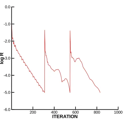
embedding solution is shown in Figure 6. In this figure, the two peaks mark the upset introduced by the adaptive grid-embedding process and shows that the rate of convergence is similar for each level of adaptation.
Supersonic Flow in a Channel with a
Circular Arc
The second case is supersonic flow with inlet Mach number of 1.4 in a channel with a %4 thick circular arc bump. The initial grid is the same as the previous case and the embedding procedure is applied twice. Figure 7 shows the generated grids and the Mach number contours for three cases with different grid configurations. The size of each cell in the fine grid configuration is the same as the smallest size in adapted grid case. The results for the embedded case that is the location and thickness of the shock waves and general flow pattern show that the same accuracy is obtained in200 400 600 800 1000
ITERATION
-6.0 -5.0 -4.0 -3.0 -2.0 -1.0 0.0
lo
g
R
comparison with the results for fine grid. Again, when the directional embedding is used, fewer wiggles are seen in the results compared to the case when both directions embedding is applied. The number of grid points for the fine grid configuration is 12545, for the embedded grid without directional embedding is 4417, and for directional embedding, this number is reduced to 3537. The required CPU time for both directions embedding is %27 of the time required for fine grid calculations. This reduces to %25 for the directional embedding case.
Supersonic Flow in a Convergent Channel
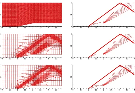
The last test case is supersonic flow in a converging channel with a 8oramp and the inletMach number of 3.0. The length of the ramp is equal to inlet height of the channel. The initial grid is 33
×
9 and the embedding procedure is applied three times. Figure 8 shows the generated grids and the Mach number contours for three cases with different grid configurations. The size of each cell in the fine uniform grid configuration is the same as the smallest size in adapted grid case. The results show that the accuracy is essentially the same as previous test cases. The number of grid points in fine grid configuration is 16705. This number for embedded grid case without directional embedding is 3941, and for directional embedding, the number is reduced to 3055. The required CPU time for both directions embedding is %24 of the time required for fine grid calculations. This0 0.5 1 1.5 2 2.5 3
0 0.5 1
0 0.5 1 1.5 2 2.5 3
0 0.5 1
0 0.5 1 1.5 2 2.5 3
0 0.5 1
0 0.5 1 1.5 2 2.5 3
0 0.5 1
0 0.5 1 1.5 2 2.5 3
0 0.5 1
0 0.5 1 1.5 2 2.5 3
0 0.5 1
reduces to %22 for the directional embedding case.
5. CONCLUSIONS
The adapted grid embedding is considered and directional and both directions subdivision are used and the results for three different cases are obtained. The results show that although the general adaptive grid embedding reduces nodes and computational time with the same accuracy when compared to fine grid configuration, but the directional embedding is more efficient. Another advantage of directional subdivision over both directions subdivision is that it produces results
with fewer wiggles around the interfaces.
6. REFERENCES
1. Berger, M. G. and Jamson, A., “Automatic Adaptive Grid Refinement for the Euler Equations”, AIAA Journal, Volume 23, (April 1985), 561-568.
2. Dannenhofer, J. F., Baron, J. R., “Grid Adaptation for the 2-D Euler Equations”, AIAA Paper, 85-0484, (January 1985).
3. Pervaiz, M. M. and Baron, J. R., “Spatiotemporal Adoption Algorithm for Two- Dimensional Reacting Flows”, AIAA Journal, Vol. 27, (October 1989), 1368-1376.
4. Dannenhofer, J. F., “A Comparison of Adaptive-Grid Redistribution and Embedding for Study Transonic
0 0.5 1 1.5 2 2.5 3 3.5 4 0
0.5 1
0 0.5 1 1.5 2 2.5 3 3.5 4 0
0.5 1
0 0.5 1 1.5 2 2.5 3 3.5 4 0
0.5 1
0 0.5 1 1.5 2 2.5 3 3.5 4 0
0.5 1
0 0.5 1 1.5 2 2.5 3 3.5 4 0
0.5 1
0 0.5 1 1.5 2 2.5 3 3.5 4 0
0.5 1
Flows”, Int. J. for Numerical Methods in Eng., Vol. 32, (1991), 653-663.
5. Burton, K. L. and Pepper, D. W., “An Adaptive Finite Element Algorithm for Compressible Flow on Workstations”, AD-Vol.23/HTD185, “Computational Techniques and Numerical Heat Transfer on PCs and Workstations”, ASME, (1991).
6. Kallinderis, Y. and Nakajima, k., “Finite Element Method for Incompressible Viscous Flows with Adaptive Hybrid Grids”, AIAA Journal, Vol. 32, (August 1994), 1617-1625.
7. Kallinderis, Y. and Baron, J. R., “Adaptation Methods for New Navier-Stokes Algorithm”, AIAA Journal, Vol. 27, (January 1989), 37-43.
8. Davis, L. D. and Dannenhofer, J. F., “Three-Dimen si o n al Ad ap t i ve Gri d -Emb ed d i n g E u l er Technique”, AIAA Journal, Vol. 32, (June 1994), 1167-1174.
9. Ni, R. H., “A Multiple Grid Scheme for Solving the Euler Equations”, AIAA Journal, Vol. 20, (November 1982), 1565-1571.
10. Yerry, M. A. and Sheperd, M.S., “A Modified Quadtree Approach to Finite Element Grid Generation”, IEEE
Graphic Journal, (1988), 31-47.
11. Saalehi, A. and Borthwick, G. L., “Quadtree and Octree Gri d Gen erat i o n ”, I n t e r n a t i o n a l J o u r n a l o f
Engineering, I. R. Iran, Volume 9, (February 1996),