Body Height Estimation System
Based on Binocular Vision
https://doi.org/10.3991/ijoe.v14i04.8400
Guangyi Yang, Deshi Li, Guobao Ru(!), Jiahua Cao, Weizheng Jin Wuhan University, Wuhan, China
Abstract—In this paper, we propose a novel approach to estimate body height from video sequences based on binocular stereo vision. Firstly, we built a parallel binocular stereo vision device and detected the foreground by using Gaussian mixture model. After shadow elimination, we proposed the contour screening algorithm to obtain the human foreground and the top point in the foreground image. Then, we detected SURF feature points in the binocular im-ages and screened them for 3 times to calculate the disparity of the head. After that, the height of human bodies can be estimated with the calibration parame-ters of binocular cameras. The experimental results demonstrate that the pro-posed method has higher measurement accuracy and spends less time which proves the effectiveness of the method.
Keywords—binocular vision, height measurement, human body, Gaussian mixture model, feature matching.
1
Introduction
Body height is an important part of the human body’s 3D information. In daily life, height measurement is one of the basic items of the physical examination. In some ticketing system (for example scenic spot tickets, train tickets), height measurement is also necessary to determine every customer’s ticket price.
to be extracted manually from a single image. Reference [4] obtains the head and feet feature points using the vertical vanishing point and constructs several constraint equations to estimate the perpendicular point, then estimates the body height. Never-theless, there are some errors with the proposed constraint equations. Refenrence [6] takes the ratios of features in the human face into account to estimate the stature of human body. But this method can only estimate the stature roughly. Reference [7] proposes a pedestrian height measurement method based on binocular vison. The 3D coordinates of the points are caculated with the background difference and the dis-parity map is based on ELAS algorithm. The human feature points are tracked with the target track algorithm to get the stable value of the stature. Reference [9] utilizes the depth camera of Kinect based on the light coding technology to obtain the dispari-ty map of the current scene, then restores the stature of the human body in the image. However, this method relies on the support of the Kinect.
In order to estimate the body height fast and accurately, we propose a new method of body height estimation based on binocular stereo vision. Firstly, subtract the back-ground information from the scene using backback-ground modeling. After shadow elimi-nation and coutour screening, we get the human foreground and the coordinate of top of the head. Then, we detect SURF feature points in binocular images and screen out correct matching points in the human foreground to caculate the head disparity. Fi-nally, the body height can be obtained with the results of camera calibration, the co-ordinate of top of the head and the head disparity.
The rest of this paper is organized as follows. In Section 2, we introduce the math-ematical model of binocular stereo vision and propose the overall measurement scheme of body height. Then, we discuss every step of the scheme in detail. In Sec-tion 3, we provide a brief introducSec-tion to Gaussian mixture model used in the fore-ground extraction and propose the contour screening algorithm to obtain the human foreground and top points. After that, in order to estimate the disparity of top points, we introduce the SURF algorithm and describe how to screen feature points to calcu-late the head disparity in Section 4. In Section 5, we discuss the calculation of body height. Finally, the experimental results are given in Section 6 and conclusions are drawn in Section 7.
2
The Measurement Scheme of Stature
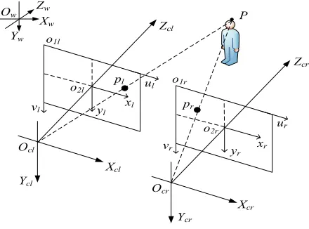
2.1 The Mathematical Model of Binocular Stereo Vision
images are rectified with Bouguet rectification method [17] to make sure the image rows between the two cameras to be aligned after rectification.
According to geometric projection relations, we can get the correspondence be-tween 2D projection points !!!! !!! in the left camera’s image pixel coordinate system
and 3D points !!!! !!! !!! in the world coordinate system as follows.
!!! !!!!!!!!!!
!!!!!!!!!!!!!!!
!!!!!!!!!
(1)
Where f is the focal length of the left camera, !!! !! is the coordinate of the prin-ciple point in the left camera’s image pixel coordinate system, !! is the baseline
length of the binocular cameras, d is the disparity of matching points. Here we define top of the head in the left image as the top point !!"#!!!"#! !!"#!. For !!"#, we need to estimate the corresponding disparity Disptop to restore its 3D information. The system uses feature matching to obtain the matching points which are the closest to !!"#. Then, calculate the disparity of the matching points Disphead to estimate the disparity of the top point Disptop.
Xcl Ycl
Zcl
Xcr Ycr
Zcr
Ocl
Ocr
P
pl
pr Zw
Ow
Yw Xw
xl yl
xr yr o2l
o2r o1l
o1r ul vl
ur vr
Fig. 1. The imaging model of the binocular stereo vision
2.2 The Measurement Process
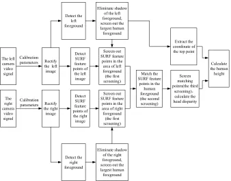
As shown in Figure 2, it’s the flowchart of measuring the height of human body. 1. Setting up a parallel binocular stereo vision system: fix binocular cameras on the
2. Calibrating the binocular cameras: Firstly, the intrinsic and extrinsic parameters of binocular cameras are obtained after the Zhang’s single camera calibration [12] and stereo calibration. Then, the image rows between two cameras are rectified to be aligned with Bouguet rectification algorithm [17].
3. Extracting human foreground and the top point’s coordinate: detect moving fore-ground in the video sequence of binocular cameras by using Gaussian mixture model [13-15], eliminate shadow and screen out the largest human contour. After that, extract the coordinate of top point.
4. Feature matching in the area of human foreground: the feature points of left-and-right images are detected by SURF algorithm [18]. Then, the SURF feature points are screened for 3 times to obtain matching points in the human foreground and We select matching points which are the closest to the top points to calculate the disparity of head.
5. Calculating the height of human body: estimate the relative height of the top point with calibration parameters, the coordinate of the top point and the disparity of head. After linear correction, the relative height and the vertical height of binocular cameras make the height of human body.
The left camera video signal The right camera video signal Calibration parameters Rectify
the left image Detect the left foreground Detect the right foreground Eliminate shadow of the left foreground, screen out the largest human foreground
Eliminate shadow of the right foreground, screen out the largest human foreground
Extract the coordinate of the top point Detect SURF feature points of the left image Detect SURF feature points of the right image Screen out SURF feature
points in the area of left foreground (the first screening)
Screen out SURF feature
points in the area of right foreground (the first screening)
Match the SURF feature
points in the human foreground (the second screening) Screen matching points(the third screening) calculate the head disparity Calculate the human height Rectify the right image Calibration parameters
3
The Human Foreground and the Top Point Extraction
The body height estimation system uses Gaussian mixture model [13-15] to do the moving foreground segmentation in the video sequence of binocular cameras. After shadow elimination and contour screening, body silhouettes and the coordinates of top points can be extracted from the binocular images.
3.1 Gaussian Mixture Model
Every pixel in images of video sequences is modeled by a mixture of K Gaussian distributions. In general, the value of K ranges from 3 to 5 in order to make the model adaptive to the lighting changes and scene changes. !!!!"! !!!!!"! !!!!"! !!!!"!! is a
particular pixel at time t. The probability of observing !!!!" is
! !!!!" ! !!!!!!!!!!"!!!!!!!"!!!!!!!"! !!!!!!"! (2)
Where !!!!!!" is the weight parameter of the ith Gaussian distrubution at time t,
!!!!!!"!!!!!!!"! !!!!!!"! is the ith Gaussian probability density function at time t, its mean
value and covariance matrix are !!!!!!" and !!!!!!". Assuming that 3 channels of RGB images are independent to each other, the covariance matrix can be expressed as !!!!!!"! !!!!!!"! !. !!!!!!"! is the variance of the ith Gaussian distribution.
Model parameters initialization.Firstly, the mean value of the 1st Gaussian
dis-tribution is initialized with the RGB value of all pixels in the first frame. Then, initial-ize K Gaussian distributions with the same weight and a high variance varInit as fol-lows.
!!!!!!"!!! (3)
!!!!!!!"! !"#$%&' (4)
Updating model parameters. Every pixel in the next frame image need to be checked against the existing K Gaussian distributions, until a match is found. A match is defined as a pixel value within 2.5 standard deviations of a distribution as Formula 5.
!!!!"! !!!!!!!!" ! !!!!!!!!!!!" (5)
Where !!!!!!!!" is the standard deviation of the ith Gaussian distribution. According to whether the match is found, the K Gaussian distributions are updated as Formula 6.
!!!!!!"! !!!!!!!!"! !!! !!!!!!!!!"!
!!!!!!"! !!!!!!!!"!! !!!!!!"! !!!!"! !!!!!!!!"
!!!!!!!"! !!!!!!!!"! ! ! !!!!!!"! !!!!!"! !!!!!!!!"!!! !!!!!!!!"!
Where ! is the learning rate which ranges from 0 to 1. The higher ! is, the faster the model is updated. M is 1 for the model which matched and 0 for the remaining models. If none of the K Gaussian distributions match current pixel value, a new Gaussian distribution would be generated to replace the nth distribution which is the
least probable. The parameters of the new Gaussian distribution is as Formula 7.
!!!!!!" !! !!!!!!"!!!!!"
!!!!!!"! ! !"#$%&' (7)
Renormalize the weights of the K Gaussian distributions after updating the model. Then, order K Gaussian distributions by the value !!!!!!"
!!!!!!".
Background estimation. As shown in Formula 8, the first B distributions are cho-sen as the background model and others model the foreground.
! ! !"# !!"#!! !!!!!!!!!!"! ! ! !!! (8)
Where ! !!! is a pre-set threshold. !! is a measure of the maximum portion of the data that can belong to pixels without influencing the background model. If matching one of the first B distributions, the current pixel value is regarded as a background pixel, otherwise as a foreground pixel.
In the contour screening algorithm, numSeq is the amount of all contours in the foreground image. areaMaxContour denotes the largest contour and contourAreaMax
denotes the maximum area value. contourAreaTemp is the temporary variable of the area and Seq denotes one of contours in the foreground image. We calculate the area of all contours to obtain the largest connected domain in the foreground image. Dur-ing the measurement, the largest connected domain is just the human foreground. Deleting smaller connected domains could prevent the human foreground from the image noise.
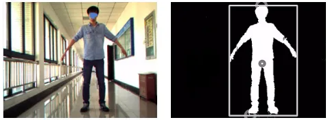
Fig. 3. Human foreground and the top point extraction
After we obtain the human foreground and contour, go through coordinates of hu-man contour and take the point which has the minimum v coordinate as the top point
!!"#!!!"#! !!"#!. We use bounding boxes and circles(gray values are 125) to mark
boundaries and top points. Human foreground image and the top point extraction are shown in Figure 3.
4
Feature Matching in the Human Foreground
In order to caculate the head disparity Disphead, the system firstly detects the SURF feature points in binocular images and screens all feature points for 3 times to obtain correct feature matching points in the head of human foreground. Then, we can esti-mate the head disparity.
4.1 SURF Feature Point Detection
SURF [18] is an speeded-up feature robust algorithm based on SIFT [19]. SURF feature points are invariant to image scaling, translation and rotation, and partially invariant to illumination change. What’s more, SURF is not only highly robust, but much faster than SIFT. SURF algorithm mainly consists of feature points detection, orientation assignment, feature points description.
Feature points detection. SURF algorithm is based on the Hessian matrix. The discriminant of the matrix can roughly screens the location of interst points in the image. Given a point X(x,y) in an image I, the Hessian matrix ! !! ! in X at scale !
! !! ! ! !!"!!!!!!!! !! !! !! !!"!!! !!
!!!!!!! (9)
Where !!!!!! !! is the convolution of the Gaussian second order derivative
!!
!!!! !!!! ! with the image I in point X and similarly for !!"!!!!! and !!!!!! !!.
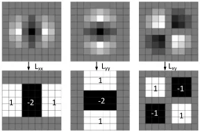
As shown in Figure 4, SURF algorithm makes use of integral image and box filter to approximate the Gaussian second order derivative for speeding up the calculation of the convolution. The approximations are denoted as Dxx, Dxy, Dyy. SURF algorithm proposes Formula 10 as the determinant of the Hessian matrix.
!"# !!""#$% ! !!!!!!! !!!!!!"!! (10)
!
"## "$$ "#$
%
% &'
%
% &%
&% % &' %
Fig. 4. Laplacian of Gaussian approximation with box filters
SURF keeps the size of the input image constant and upscales the size of box fil-ters to construct the image pyramid. The initial scale layer of the image pyramid is the convolution of the original image and the 99 box filters which correspond to scale
! ! !!!. Subsequent layers are obtained by filtering the original image with the box filters the size of which gradually becomes bigger. In order to maintain the structure of box filters, the smallest step size of two consecutive box filters must be 6.
According to Formula 10, the local extremum could be detected as an interest point. Then, a non-maximum suppression is applied in the scale space to compare the interest point with its 26 neighbours and only the maximum and minima can be re-garded as the feature point. Finally, interpolate the nearby data of the feature point in the scale space to find the location to subpixel accuracy.
Orientation assignment. After locating all feature points, SURF calcaulates the Haar wavelet responses of size 4! within a radius of 6! of the feature point. Further-more, the responses are weighted with the Gaussian the standard deviation of which is
2.5!. Rotate a circular sector covering an angle of !
! to calculate the sum of the Haar
wavelet responses around the origin and choose the longest vector as the orientation of the feature point.
de-notes the Haar wavelet response in horizontal direction and dy denotes the Haar wave-let response in vertical direction. The responses need to be weighted with a an!!!!"!. Then, in each subregions, dx, dy and the absolute values |dx|, |dy| are summed up to form a four-dimensional descriptor vector as follows.
! ! !!"#! !"#! ! !" ! !!!"!! (11)
There are 4!4 subregions for each feature point which results in a descriptor vector of length 64.
4.2 Three Times Screening of the Feature Points
In the actual measurement of body height, we only want to get matching points in the human foreground and calculate the head disparity. Therefore, it’s necessary to screen out correct matching points from all detected feature points.
The first screeningThe system uses white pixels (gray values are 255) to mark the foreground region, while using black pixels (gray values are 0) to mark the back-ground region. Then, the system can determine whether the feature point belongs to the foreground by the gray value of its coordinate in the foreground image. Set the coordinate of the feature point as X(xk,yk), and gvf(xk,yk) denotes the gray value of the feature point’s coordinate in the foreground image. If gvf(xk,yk)=255, X(xk,yk) belongs to the foreground region and we retain the feature point; if gvf(xk,yk)!255, X(xk,yk) belongs to the background region, so we exclude the feature point. As shown in the following three sets of images, Figure 5(a) is the left and right view of the original feature point images before screening, Figure 5(b) is the extracted foreground image of the corresponding frame from the scene, Figure 5(c) is the feature point images after the first screening.
(a) The original feature points image before the first screening
(c) The feature points image after the first screening Fig. 5. The first screening effect
As shown in Figure 5, taking the test images for example, 1819 SURF feature points are detected in the left original image, 1814 in the right original image. After the first screening, 243 feature points in the left human foreground and 231 feature points in the right human foreground are reserved.
The second screening. The second screening is the process of feature matching. The system takes an effective method of feature matching by comparing the Euclide-an distEuclide-ance of the closest neighbor to that of the second-closest neighbor [19]. Set that
Pliis the ith feature point of the left image, Prj is the jth feature point of the right image, the descriptor vectors of these two feature point are Descrliand Descrrj. The Euclidean distance of these two feature point is defined as follows.
! !!"! !!" ! !!!!!!"#$%!"!! !"#$%!"!!! (12)
Where m is the dimensions of the descriptor vector, !"#$%!"! and !"#$%!"! are
re-spectively the kth element of the descriptor vector of P
li and Prj. Set that ND is the closest distance, NND is the second closest distance. The ratio of distances is defined as !"#$% !!!"!". ! is set as the threshold. Only when !"#$% ! ! can the match be considered reliable, otherwise unreliable. The principle of the matching method is that we only match two feature points when ND is much smaller than NND which can lower the false matching rate effectively. In the experiment, we set ! as 0.6. The second screening effect is shown in Figure 6.
Fig. 6. The second screening effect
The third screening. The system is based on the parallel binocular stereo vision. Therefore, after stereo recitification, the binocular images should reside in the same plane with image rows aligned into a frontal parallel configuration. Taking the error of the stereo rectification into account, the absolute value of the v-axis coordinate difference between a pair of matching points should be 0 or few pixels unit which we define as !" ! !!"! !!" . Xkl(xkl,ykl) and Xkr(xkr,ykr) denote the coordinates of the matching points after the second screening and vThresh denotes the screening thresh-old of the matching points. If !"! !!!!!"!, we retain the matching points; If
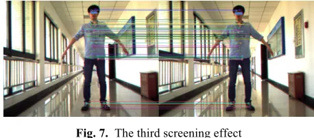
!"! !!!!"#!, we delete the matching points. In the experiment, vThresh is equal to 2. The third screening effect is shown in Figure 7.
Fig. 7. The third screening effect
As shown in Figure 7, after screening for 3 times, there are 45 matching points left. Compared with the second screening, the third screening eliminates 4 error matching points. It can be seen that screening for 3 times not only eliminates the matching points in the backgournd region which we are not intrested in, but greatly eliminates the error matching points in the human foreground region.
After feature matching in the human foreground, the system screens out the match-ing points which are the closest to the top of head !!"# !!"#! !!"# as the head
match-ing points. !!! !!!! !!! !and !!! !!!! !!! denote the matching points of the head.
Then, the head disparity is:
!"#$!!"# ! !!!! !!! (13)
5
The Calculation of Body Height
According to Formula 1, the coordinate of the top point in the world coodinate sys-tem (the left camera coordinate syssys-tem) can be restored with the calibration parame-ters, the coordinate of !!"#!!!"#! !!"#! and the head disparity Disphead. Because the system is used to measure the body height, we only concern about the Yw-axis coordi-nate values Ymanwhich is
!!"#!!!!!"#$!"#!!!!"#!!!!! (14)
!!"#!!!!"#! ! !! (15) Where !! is the vertical height of the binocular cameras. In fact, it’s difficult to make the Yw-axis vertical to the horizontal ground perfectly. Hence, we need to cor-rect Yman linealy before using Formula 15 to caculate the body height.
6
Experiment Results and Analysis
We do the experiment indoor where the illumination is stable and the floor is flat. In the experiment, !!!"#!! denotes the vertical height between top of the head and the origin of the left camera coordinate system. Firstly we take 9 people whose body height we already know to linearly fit !!!"#! and !!!"#!!. After obtaining fitting parameters, the system can linearly corrects !!!"#! and estimate the body height.
Here we take another 10 people at random to estimate their body height. The experi-ment is based on Window7 operating system, using Visual Studio 2013 and OpenCV 2.4.9 as software platforms. The computer processor is Intel Core i7-3520M, clocked at 2.90 GHz. The resolution of the test video is 640*480. The camera model is SUNTIME 300C from Taiwan. The mapping table of !!!"#! and !!!"#!! is shown in Table 1.
Table 1. Mapping table of !!!"#! and !!!"#!!
No. !!!"#! (mm) !!!"#!! (mm) No. !!!"#! (mm) !!!"#!! (mm)
1 971 1053 6 1043 1115
2 890 990 7 969 1064
3 924 1020 8 755 855
4 948 1025 9 842 935
5 857 945
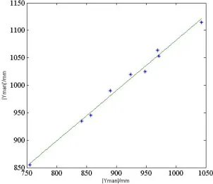
We linearly fit !!!"#! and !!!"#!! in the MATLAB to weaken the effect of the
camera coordinate system which is not vertical to the horizontal ground perfectly and the systematic error. The linear fitting of !!!"#! and !!!"#!! is shown in Figure 8.
After linear fitting, the correspondence relationship of !!!"#! and !!!"#!! can be represented with a linear equation ! ! !" ! !. In the experiment, k=0.9171 and
b=164.7176. Then, we linearly correct !!!"#! to get the value of !!!"#!!. As shown in
Formula 15, the body height !!"# can be estimated by !!"#! !!!"#!!!!!. In the experiment, !! is set as 710 mm. Then, we make use of the system to estimate the body height of another 10 people and each was measured for three times. The meas-urement results are shown as Table 2.
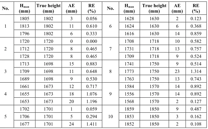
Table 2. The measurement data of stature and error analysis
No. (mm) Hman True height (mm) (mm) AE (%) RE No. (mm) Hman True height (mm) (mm) AE (%) RE
1
1805 1802 3 0.056 6
1628 1630 2 0.123 1813 1802 11 0.610 1624 1630 6 0.368 1796 1802 6 0.333 1616 1630 14 0.859
2
1720 1720 0 0.000 7
1708 1718 10 0.582 1712 1720 8 0.465 1731 1718 13 0.757 1728 1720 8 0.465 1709 1718 9 0.524
3
1713 1698 15 0.883 8
1741 1750 9 0.514 1709 1698 11 0.648 1773 1750 23 1.314 1689 1698 9 0.530 1763 1750 13 0.743
4
1661 1673 12 0.717 9
1584 1570 14 0.892 1655 1673 18 1.076 1556 1570 14 0.892 1653 1673 20 1.196 1568 1570 2 0.127
5
1702 1701 1 0.059 10
1859 1850 9 0.487 1706 1701 5 0.294 1853 1850 3 0.162 1677 1701 24 1.411 1852 1850 2 0.108
As shown in Table 2, in the experiment, the accuracy of measurements shows the high precision and the absolute error(AE) is within the range of 24mm, the relative error(RE) is within the range of 1.5%. The error is mainly from the disparity differ-ence between Disptop and Disphead which are close to each other but not the same,
because Disphead depends on the SURF matching points in the human foreground and
we use it to estimate the disparity of the top points Disptop. What’s more, the distance
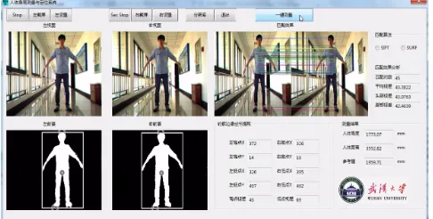
Fig. 9. The interface of body height estimation system
7
Conclusion
In this paper, we propose a new kind of body height estimation system based on binocular vision. First, the system uses the Gaussian mixture model to extract the foreground. After shadow elimination and contour screening, the human foreground and the coordinate of the top point are obtained. Then we detect the SURF feature points in the binocular images and screen them for 3 times to caculate the head dispar-ity. Combined with the calibration parameters, the body height can be estimated. Experiments show that the system has relatively good accuracy and stablity. It also takes relatively short time for every measurement. The system meets the basic meas-uring needs of the body height in the stable measurement circumstances.
8
Acknowledgements
This paper is supported by the National Natural Science Foundation of China (NSFC) (No. 61671333, 61571334).
9
References
[1]M. X. Jiang, P. C. Wang, H. Y. Wang. “Height Estimation Algorithm Based on Visual Multi-Object Tracking”, Acta Electronica Sinica, vol. 43, no. 3, (2015), pp. 591-596. [2]A. Criminisi, I. Reid, A. Zisserman. “Single View Metrology”, International Journal of
Computer Vision”, vol. 40, no. 2, (2000), pp. 123–148. https://doi.org/10.1023/A:10 26598000963
[3]C. Benabdelkader, Y. Yacoob. “Statistical Body Height Estimation from a Single Image”, IEEE International Conference on Automatic Face & Gesture Recognition, (2008), pp. 1-7.
https://doi.org/10.1109/AFGR.2008.4813453
[4]Q. L. Dong, Y. H. Wu, Z. Y. Hu. “Video-based Real-time Automatic Measurement for the Height”, Acta Automatica Sinica, vol. 35, no. 2, (2009), pp. 137-144.
[5]J. Cai, R. Walker. “Height Estimation from Monocular Image Sequences Using Dynamic Programming with Explicit Occlusions”, IET Computer Vision, vol. 4, no. 3, (2010), pp. 149–161. https://doi.org/10.1049/iet-cvi.2009.0063
[6]Y. P. Guan. “Unsupervised Human Height Estimation from a Single Image”, Journal of Biomedical Science and Engineering, vol. 2, no. 6, (2009), pp. 425–430.
https://doi.org/10.4236/jbise.2009.26061
[7]R. Q. Du, Y. Z. Gu, C. Zhang, Y. G. Wang. “Method of Pedestrian Height Measurement Based on Binocular Stereo Vision”, Information Technology, vol. 24, no. 1, (2016), pp. 91-95.
[8]E. Jeges, I. Kispal, Z. Hornak. “Measuring Human Height Using Calibrated Cameras”, Proceedings of the 2008 Conference on Human Systems Interactions, (2008), pp. 755-760
https://doi.org/10.1109/HSI.2008.4581536
[9]C. S. Zhou, Z. Shi. “Design of Height Measurement System Based on the Depth Image”, Journal of Guilin University of Electronic Technology, vol. 33,no. 3, (2013), pp. 214-217 [10]Y. M. Mustafah, R. Noor, H. Hasbi, A.W. Azma. “Stereo Vision Images Processing for
Real-time Object Distance and Size Measurement”, International Conference on Computer and Communication Engineering, (2012), pp. 659-663. https://doi.org/10.1109/ICCCE.201 2.6271270
[11]C. Madden, M. Piccardi. “Height Measurement as a Session-based Biometric for People Matching across Disjoint Camera Views”, Image & Vision Computing New Zealand, (2005), pp. 29.
[12]Z. Zhang. “A Flexible New Technique for Camera Calibration”, Transactions on Pattern Analysis and Machine Intelligence”, vol. 22, no. 11, (2000), pp. 1330-1334.
https://doi.org/10.1109/34.888718
[13]C. Stauffer, W. E. L. Grimson, “Adaptive Background Mixture Models for Real-time Tracking”, Proceedings of IEEE Conference on Computer Vision and Pattern Recognition, (1999), pp. 246-252. https://doi.org/10.1109/CVPR.1999.784637
[14]C. Stauffer, W. E. L. Grimson. “Learning Patterns of Activity Using Real-time Tracking”, IEEE Transactions on Pattern Analysis and Machine Intelligence, vol. 22, no. 8, (2000), pp. 747-757. https://doi.org/10.1109/34.868677
[15]Z. Zivkovic. “Improved Adaptive Gaussian Mixture Model for Background Subtraction”, Proceedings of the 17th International Conference on Pattern Recognition, (2004), pp. 28-31. https://doi.org/10.1109/ICPR.2004.1333992
[16]T. Horpraset, D. Harwood, L. Davis. “A Statistical Approach for Real-time Robust Back-ground Subtraction and Shadow Detection”, IEEE ICCV Frame Rate Workshop, (1999), pp. 1-19.
[17]Bouguet J. “Camera Calibration Toolbox for Matlab[DB/OL]”. http: // www. vision. cal-tech. edu/ bouguetj/ calib_doc, (2010).
[18]H. Bay, T. Tuytelaars, L. van Gool. “SURF: Speeded Up Robust Features”, Computer Vi-sion and Image Understanding, vol. 110, no. 3, (2006), pp. 404-417.
https://doi.org/10.1007/11744023_32
[19]D. Lowe. “Distinctive Image Features from Scale-Invariant Keypoints”. The International Journal of Computer Vision, vol. 2, no. 60, (2004), pp. 91-110.
https://doi.org/10.1023/B:VISI.0000029664.99615.94
10
Authors
Guangyi Yang, he received his M.Sc. degree in Electronic Engineering from Wu-han University, China in 2008. He is currently an engineer in the School of Electronic Information, Wuhan University. His research interests involve in high frequency circuit and image processing, etc.
Deshi Li, he received the phD degree in Computer Science from Wuhan Universi-ty, China in 2001. Dr. Li is currently a professor and dean in the School of Electronic Information, Wuhan University. His research is involved in wireless sensor networks, networked robots, wireless communication, etc.
Guobao Ru, he received his B.S. degree in Electronic Engineering from Wuhan University, China in 1986. Dr. Ru is currently a professor in the School of Electronic Information, Wuhan University. His research is involved in wireless communication and machine vision, etc.
Jiahua Cao, he is currently studying for his B.S. degree at the school of Electronic Information in Wuhan University, China. His research interests include image pro-cessing and pattern recognition.
Weizheng Jin, he received his M.Sc. degree in Electronic Engineering from Wu-han University, China in 1991. He is currently an associate professor in the School of Electronic Information, Wuhan University. His research is involved in high frequency circuit and image processing, etc.