Longitudinal Multivariate GARCH Model with
an Application to Highly Dimensional Intraday
Stock Returns and Electricity Prices
1Edison G. Yu
October 2006
Abstract
This paper examines the intraday heteroskedasticity of the volatility and correlation of financial time series by using the longitudinal multivariate GARCH (LMGARCH) model. Two versions of the LMGARCH model are examined, with one assuming a constant correlation matrix and the other allowing the conditional correlation matrix to be time-varying. A banded precision matrix of the disturbances is employed in the model to allow the modelling of highly dimensional intraday financial time series. Reparameterization is used to allow a completely unconstrained optimization of the likelihood function during estimation. Then, a simulation study is used to demonstrate the reliability of both the model and the inferential procedures. The application of the model to the BHP intraday stock returns shows noticeable intraday periodicity in the volatility and correlation. In particular, the volatility is highest at the beginning and lowest in the middle of each day. Negative serial correlation during the middle of day is captured, which confirms previous empirical studies. Then, the model is applied to modelling the intraday wholesale electricity prices of New South Wales. In addition to the intraday periodicity in the volatility, conditional correlations of the intraday electricity prices are also found to be time-varying.
Keywords: Longitudinal MGARCH; Intraday heteroskedasticity; Intraday periodicity; High frequency; Reparameterization; BHP stock returns; Electricity prices
1
1
Introduction
The modelling of volatility of financial returns is used extensively for hedging, risk-management, and other financial decision making. One of the most important stylized facts about financial data is that it tends to exhibit volatility clustering, where high volatilities are more likely to be followed by high volatilities, and low volatilities with low volatilities. The introduction of the univariate GARCH model (Engle, 1982 and Bollerslev, 1986) and its many variations was a significant step forward in modelling time-varying volatility. Despite the increasing popularity of the stochastic volatility (SV) model (Taylor, 1986) as an alternative, the GARCH family of models still remains the most popular choice for the modelling of volatility of financial assets in practice. The popularity of the GARCH model is mainly due to its simple specification and ease of estimation using maximum likelihood based procedures.
In most situations, the GARCH specification has been applied to low frequency financial data, for example daily stock returns, assuming there is no intraday heterogeneity in the data. However, many studies have found that the assumption is rejected by real data. (see Andersen and Bollerslev, 1997, for example) Also, in the finance literature, intraday volatilities have been shown to have a diurnal pattern, with higher volatilities at the beginning and the end of each day. Thus, estimating a single univariate GARCH model, while ignoring the intraday heterogeneity, is potentially a major flaw and may lead to incorrect inference. In this paper, I attempt to incorporate intraday heterogeneity through a formal model and apply it to two intraday series.
The aim of this paper is threefold. Firstly, the intraday high-frequency data is studied in a longitudinal framework, with data recorded at the same time each day taken to be a separate time series. The intraday periodicity is then explicitly addressed using a multivariate GARCH (MGARCH) model. Secondly, This paper aims to extend the constant conditional correlation MGARCH (CCC-MGARCH) model (Bollerslev, 1990) and the dynamic conditional correlation MGARCH (DCC-MGARCH) model (Engle, 2002) to the longitudinal case. Here, a parsimonious structure for the precision matrices of the disturbances is employed. This allows the modelling of intraday longitudinal data in high frequency, which is difficult for the original MGARCH models. It will be seen that the LMGARCH model proposed in this paper has the advantage in terms of ease of estimation in the context for intraday longitudinal data, since the number of the parameters of the model only increases linearly with the dimension of the model. Thirdly, the LMGARCH model will be applied to real data in an effort to demonstrate (1) the reliability of the inferential procedures, (2) the usefulness of the model, and (3) distinct intraday patterns that can arise in high-frequency financial data.
2
The GARCH Models
2.1 Univariate GARCH Model
While the marginal volatility of financial returns is usually thought to be a constant, the conditional volatility is often assumed to be time-varying in a smooth manner, which is reflected in the data by the clustering of volatility. Engle (1982) addressed this stylized fact through a systematic model – the ARCH model. This model specifies a time series { }yt to be the sum of a conditional mean { }t and an innovation term { }at , wheret can be a function of both exogenous variables and past values of yt . A typical specification for t is an autoregressive moving average (ARMA) model. The innovation conditioned on the information set Ft1{yt1,t1,yt2,t2,...} up to time
1
t is assumed to be normally distributed in Engle’s original model. However, this Gaussian assumption can be easily replaced by other distributions (see Bollerslev (1987) for example). The ARCH model is defined as in equations (2.1) and (2.2).
, t t t
y a (2.1)
2 1
2 2
1 1
| (0, ),
,
t t t
P
t i t
i
a F N
a
(2.2)where t2 is the conditional variance of the innovation at time t , and i are coefficient parameters, and P is the predefined order of lags in the squared past innovations to be included. This model was generalized by Bollerslev (1986) to the GARCH model:
2 2 2
1 1
1 1
Q P
t i t j t
i j
a
, (2.3)where j, for all j , are coefficient parameters, and Q is the predefined lag length of past conditional variances in the model. Both the ARCH and the GARCH model specify a deterministic volatility function of past information, which allows the model to capture the clustering of volatility. In order to ensure positive volatility at each time period, it is usually assumed that 0, 0i and j 0 for all i and j. Also, the
restriction
1 1
1 Q
P
i j
i j
is assumed throughout, which ensures the series 2stationary. The estimation of the model is usually carried out through MLE. For a more detailed discussion of the ARCH and GARCH model and their numerous variations, see Bera and Higgins (1993).
2.2 The MGARCH Model
2.2.1 Definition
Because there is strong correlation in both the first and second moments of stock returns, modelling the return series in a multivariate framework is more appropriate. This allows the study of the co-movement of the time-varying volatilities and the potential evolution of correlations between them. Recently, MGARCH modelling has become a fast growing area in financial econometrics and a survey paper on MGARCH model has been recently provided by Bauwens et al. (2006). Also refer to Tsay (2005) for a textbook treatment.
The mean equation of the MGARCH model is a straightforward extension of the univariate case; scalars are simply replaced with vectors:
, t t t
y a (2.4)
where yt , t , and at are now all N1 vectors, and N is the dimension of the multivariate model.
The volatility equation is as follows:
1
2 ,
t t t
a H (2.5)
where,
( ) 0,
( ) .
t
t N E
Var I
(2.6)
Here, Ht is an NN positive definite matrix, and tis an N1 white noise random vector. The following shows that t and Ht are the first and second conditional moments of yt.
1 2
1 1 1
( ) ( ) ( )
( )
t t t t t t
t t t t
E y F E F E a F
H E
1 1
2 2
1 1
2 2
1 1 1 1
1
( ) ( ) ( ) ( , )
( )( ) '
t t t t t t t t t
t t t t
t N t t
Var y F Var F Var a F Cov a F
H Var F H
H I H H
(2.8)
While the conditional mean,t, can be specified in a variety of ways, one of the most popular choices is a vector autoregressive (VAR) model. The specification of Ht varies according to different types of MGARCH models. Bauwens et al. (2006) categorize the many possible MGARCH models into three groups according to the different specification of Ht : (1) Ht is a direct generalization of the univariate GARCH model; (2) Ht is a linear combination of univariate GARCH models; and (3) Ht is a nonlinear combination of univariate GARCH models.
Across all the models, the most well-known are the Vech, BEKK, CCC-MGARCH and, more recently, DCC-MGARCH models. Without loss of generality, the discussion of these models will be restricted to generalizations of the GARCH(1,1) case. The choice of this order can be justified on the grounds that GARCH(1,1) or MGARCH(1,1) have been found to be adequate in most applications.
2.2.2 Vech Model
The most general MGARCH is the Vech model (Bollerslev et al., 1988), which is a direct generalization of the univariate GARCH model.
'
1
( t) ( ) ( t t) ( t ),
vech H vech W A vech a a B vech H (2.9)
where vech( ) denotes an operator that stacks the lower triangular portion of a matrix to be a vector, W is a positive definite NN matrix, and A and B are both r r matrices with rN N( 1) / 2.
Engle and Kroner showed that, as long as the absolute value of all eigenvalues of
plus the large number of parameters of the model (N N( 1)( (N N 1) 1) / 2) means that the model is effectively restricted to use only in bivariate cases2.
2.2.3 BEKK Model
To solve the difficulty of ensuring Ht is positive definite, Engle and Kroner (1995) propose the BEKK model (after Baba, Engle, Kraft and Kroner), where
'
1
' ' ' .
t t t t
H GG A a a AB HB (2.10)
Here,G, A, and Bare all NN matrices, but G is lower triangular.
While Ht is guaranteed to be positive definite, the number of parameters in the model is still large at N(5N1) / 2. Moreover, the parameters in the BEKK model cannot be easily interpreted due to the complicated matrix multiplications.
2.2.4 Constant Conditional Correlation MGARCH (CCC-MGARCH)
The constant conditional correlation, or CCC, MGARCH model was firstly proposed by Bollerslev (1990) together with an application to study the volatility structures of foreign exchange rates of five European currencies.
1 2
2 2 2
1 1
,
( , ,..., ), , t t t
t t t Nt
it i i it i it
H C
diag
a
(2.11)
where C is an NN constant correlation matrix and tis an NN diagonal matrix, whose diagonal elements each follow a univariate GARCH model.
Note that although the correlation matrix is constant, the covariance matrix Ht still follows a dynamic structure through the time-varying conditional variances t. The constant correlation specification allows the number of parameters to be reduced to
( 5) / 2
N N , which is smaller than the BEKK model. The positive definiteness of the covariance matrix Ht is ensured by having a positive definite correlation matrix C.
2
2.2.5 Dynamic Conditional Correlation MGARCH (DCC-MGARCH)
One of the major critiques of the CCC-MGARCH model is its assumption of a constant correlation matrix, which seems unreasonable in many applications using real data (see Christodoulakis and Satchell, 2002 and references therein). Recently, the CCC-MGARCH model has been extended to a new class of models entitled dynamic conditional correlation, or DCC, MGARCH models. Two slightly different DCC-MGARCH models were independently developed by Tse and Tsui (2002) and Engle (2002). In general, the DCC-MGARCH model extends its CCC predecessor by permitting the correlation matrix to also vary over time, so that
, t t t t
H C (2.12)
1 2
( , ,..., ), t diag t t Nt
(2.13)
2 2 2
1 1. it i iait i it
(2.14)
The two DCC-MGARCH models differ only in the specification of Ct:
a) DCCT (Tse and Tsui, 2002)
1 2 1 1 2 1
(1 ) ,
t t t
C C C (2.15)
where 1 and 2 are non-negative scalars with the constraint 1 2 1 for stationarity, and C is a symmetric NN positive definite parameter matrix with ones on its main diagonal. The NN matrix t1 is the sample correlation matrix of the standardized innovations between time tMand t1, where M is chosen by the user. The ,i jth element of t1 can be written as follows:
, , 1
, 1
2 2
, ,
1 1
,
/ . M
i t m j t m m
ij t
M M
i t m j t m
m m
it it it
where a
(2.16)1 ' 1 1 1 1 1 1
2 2
1 1 1, 1 ,
1 1 1
,
( ,..., ),
( ,..., ), ( ,..., ) '. t t t t t
M M
t m t m m N t m
t t t M t t Nt
B E E B
B diag
E where
(2.17)
Under this specification, Ct is guaranteed to be positive definite. The formulation of the Ct is an analogue of a GARCH equation with an equally weighted sum of past correlation coefficients as the innovations. However, this is also a weakness of the model, since it is sometimes difficult to justify the use of equal weights. Another DCC model, proposed by Engle (2002) managed to avoid the arbitrary choice of the weights by using a different specification of Ct.
b) DCCE (Engle, 2002)
1 1
2 2
[ ( )] [ ( )] ,
t t t t
C diag Q Q diag Q (2.18)
'
1 2 1 1 1 2 1
(1 ) ,
t t t t
Q S Q (2.19)
where 1 and 2 are also non-negative scalars satisfying 1 2 1 for stationarity and S is an NN unconditional covariance matrix oft (also see Engle and Sheppard, 2001). The idea behind this model is that the matrix Qt follows a GARCH like equation and the normalization of Qtthrough pre and post multiplying [ ( )] 12
t diag Q
ensures that Ct is a proper correlation matrix for each time period t. This specification does not restrict the conditional correlation to be a weighted sum of past correlations. Due to this flexibility, the DCCE model will be adopted in this paper to develop the
DCC-LMGARCH model.
One useful property of the DCC model is that it nests the CCC model. Then, the constant correlation hypothesis can be checked through testing 1 2 0 or
1 2 0
.
2.3 Alternative Model
usually follows a Gaussian distribution, in the volatility equation, instead of the deterministic volatility equation in a GARCH model. The basic MSV model was introduced by Harvey et al. (1994), which specifies a multivariate normal distribution for the stochastic terms in all the volatility equations in the model. This extra set of stochastic driving factors in the volatility equations provides the model with a greater degree of flexibility.
Another advantage of the MSV model is its close link to the continuous time model, which is often used in the methodological finance literature. The MSV model can be written as a discretized version of a two factor continuous time model, with a mean reverting multivariate Ornstein-Uhlenbeck process for volatility (see Pitts, 2004 for example). This gives a nice interpretation to the MSV model and allows the MSV model to handle problems such as extremely high-frequency data, missing data, and non-synchronous trading relatively easily. The GARCH model, on the other hand, is purely a time series model for equally spaced data and unlike the SV model, a continuous time analogue of the GARCH process is difficult to derive. Recently, bridging the gap between the discrete GARCH and the continuous time GARCH process is becoming an active area of research. A brief discussion of the diffusion limit of the GARCH model is provided in Appendix B, but it is currently unknown if a similar limiting model is derivable for the MGARCH models discussed in the previous sections.
3
Longitudinal MGARCH Model
When the number of elements in the vector yt, N , is large, even the CCC and DCC MGARCH models are highly parameterized. If the specification for the conditional volatility follows a GARCH(1,1) for each series, the number of parameters of the CCC model is N N( 5) / 2, and that of both types of DCC models is (N1)(N4) / 2, two more than the CCC model. Thus the number of parameters increases quadratically as the dimension of the model increases. But for longitudinal data, it is possible to reduce the number of parameters, so that they go up only linearly in N.
In modelling longitudinal data, yt in the MGARCH model mentioned before becomes a vector of contiguous elements of the same series observed at different times of the day. In other words, the subscript i in equation (2.13) indicates the time of day, while the subscript t indicates the day on which the data is observed. The reduction of the number of parameters can be achieved by imposing a band structure on the precision matrix. For the CCC model, the restriction is imposed on the inverse of C in (2.11), and for the DCCE model, the restriction is on the inverse of S in (2.19). In other
words, 1
C and 1
S are assumed to be banded with bandwidth k. Two points should be noted here. Firstly, though the precision matrices are banded, the correlation matrixC
and the covariance matrixS are not banded. The banded 1
C and 1
S correspond to assumptions of lag k intraday autocorrelation and that the process is Markovian intra day with lag length k. Secondly, the off-diagonal entries in the banded precision matrix do not have to be the same. This is different from a simple autoregressive model, which has off-diagonal entries in the precision matrix that are the same at each band. Such a model with flexible entries at each band is called an ante-dependence model (Gabriel, 1962). The concept of this model has been adopted and extended by Pourahmadi (1999, 2000) to conduct mean-covariance modelling. The justification of using a band structure in modelling stock returns and electricity prices will be provided in Chapter 6 and Chapter 7, respectively. The following equations summarize the CCC-LMGARCH(1,1) and DCC(1,1)-CCC-LMGARCH(1,1) models.
1 2
1 2
2 2 2
1 1
(0, )
( , ,..., ) t t t
t t t
t N
t t t Nt
it i i it i it
y a a H N I diag a (3.1) CCC-LMGARCH(1,1) 1
is a correlation matrix
is a banded matrix with bandwidth
t t t
H C
C
C k
(3.2) DCC(1,1)-LMGARCH(1,1) 1 1 2 2 '
1 2 1 1 1 2 1
1
[ ( )] [ ( )]
(1 )
is a covariance matrix
is a banded matrix with bandwidth
t t t t
t t t t
t t t t
H C
C diag Q Q diag Q
Q S Q
S S k
(3.3)
The “(1,1)” after the “LMGARCH” indicates that a GARCH(1,1) process is used for the variance of each series and the “(1,1)” after the “DCC” means that only one lag in the outer product of the standardized innovation t and one lag in Qt is used for the dynamic conditional correlation model. As suggested by many applications in practice, the (1,1) structure is adequate and will be adopted in this paper. The stationarity conditions of the models are the similar as in the CCC and DCC MGARCH models discussed in the previous chapter. Moreover, because the time series {yit} is split up into contiguous longitudinal vectors, the elements of which follow stationary univariate GARCH processes, the entire series is also stationary. Interestingly, this is the case regardless of the value of the elements of C or Ct.
4
Methods of Estimation and Inference
4.1 Asymptotical Independence of the Mean and Volatility
Equation
As mentioned in the Chapter 2, estimation of MGARCH models can be conveniently conducted through maximum likelihood. It is also known that for the univariate GARCH model, the conditional mean equation and the conditional volatility equation are asymptotically independent. In other words, the information matrix of the full log-likelihood function can be shown to be block-diagonal (Bollerslev, 1986 and Engle, 1982). This independence allows separate estimations of the mean and volatility equations without loss of efficiency. Thus, in practice, the mean equation is usually estimated first, and then the volatility equation is estimated in a second step using the residuals from the mean equation.
The extension of this independence idea to the LMGARCH model is natural, since the volatility equation for each time series follows a univariate GARCH, though no formal research has been done in the literature. So in this paper, there are three steps in estimating an LMGARCH model with a regression conditional mean t. The first step is to obtain OLS estimates of the mean equation and the innovations at. Using these innovations as the prefiltered data, the second step uses maximum likelihood to obtain both consistent and efficient estimates of the parameters in the LMGARCH model. Conditional on the estimates obtained in the second step, the third step involves maximizing the full log-likelihood function by estimating both consistent and efficient estimates for the parameters in the regression mean equation.
4.2 The Log-likelihood Function
As shown in (2.7) and (2.8), tand Ht are the first and second conditional moments of t
y . If we assume further that yt follows a normal density3, conditional on tand Ht, then:
1 ( , ).
t
t t t
y F N H
So the conditional log-likelihood function at time t is:
3
' 1
1 1
( ) log(2 ) log( ) ,
2 2 2
t t t t t
N
l H a H a
where at ytt and N is the number of cross sections or dimensions of the MGARCH model. The joint log likelihood can then be obtained by repetitive use of the properties of conditional densities:
' 1
1
1 1 1
1 1
( ) ( ) log(2 ) log( ) log( ( )),
2 2 2
N T T
t t t t t
t t t
NT
l l H a H a f y
where f y( )1 is the density of the initial observation y1. In financial time series analysis, 1
( )
f y is usually dropped to simplify the expression of the likelihood. This is not a problem when the sample size T is large, which is usually true for financial data. So the log likelihood function becomes:
' 1
1 1
1 1
( ) log(2 ) log( ) ,
2 2 2
T T
t t t t
t t
NT
l H a H a
(4.1)where:
;
: depends on the specification of the MGARCH model; : dimension of the MGARCH model;
: total time periods of the data. t t t
t
a y
H
N
T
Since Ht is usually a complicated function of the parameters, an analytical solution to the optimization problem is usually not available. Numerical optimization is therefore used to obtain the maximum likelihood estimates.
However, there are two complications that arise prior to the use of numerical optimization when maximizing the log-likelihood: (1) curse of dimensionality, and (2) imposing restrictions on the parameters.
4.3 Curse of Dimensionality
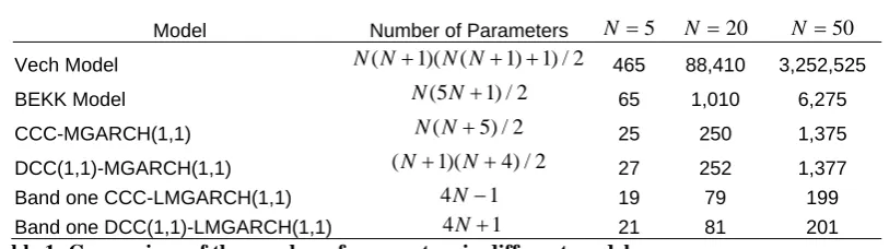
model increases. Table 1 provides a comparison of the number of parameters in different models. For example, when the dimension of the model is 20, the number of parameters to be estimated in a CCC-MGARCH(1,1) model will be 250 while that in a DCC(1,1)-MGARCH(1,1) model will be 252. And those numbers will go up to 1,375 and 1,379 respectively when the dimension is 50. This rapid increase in the parameterization of the model will lead to instability and intractability in the numerical optimization and will eventually prevent the model from being estimated when the number of parameters is greater than the number of observations.4 This curse of dimensionality means that, until recently, most applications of MGARCH models are constrained to relatively low dimensions. For example, Bollerslev et al.(1988) estimated a 3 dimension Vech model, Bollerslev (1990) estimated a CCC-MGARCH model with 4 dimensions, Karolyi (1995) used a bi-variate BEKK model, Attanasio (1991) estimated a 6 dimension Vech model, and BEKK models with 3 to 5 dimensions are used in Kearney and Patton (2000).
Model Number of Parameters N 5 N 20 N 50
Vech Model N N( 1)( (N N 1) 1) / 2 465 88,410 3,252,525
BEKK Model N(5N1) / 2 65 1,010 6,275
CCC-MGARCH(1,1) N N( 5) / 2 25 250 1,375
DCC(1,1)-MGARCH(1,1) (N1)(N4) / 2 27 252 1,377
Band one CCC-LMGARCH(1,1) 4N1 19 79 199
Band one DCC(1,1)-LMGARCH(1,1) 4N1 21 81 201
Table 1: Comparison of the number of parameters in different models
For longitudinal data, as firstly mentioned in Chapter 4, a band structure can be imposed on the precision matrix of the MGARCH model, which will result in the number of parameters only increasing linearly as the dimension increases. For the same example in Table 1, if the dimension of the model is 50, the band one LMGARCH model will only have 199 and 201 parameters for the CCC and DCC specification, respectively. Given this reduced number of parameters, a model with a much higher dimension can be estimated.
4
4.4 Restrictions on Parameters
As discussed briefly in Chapter 4, there are two sets of restrictions on the parameters. The first group relates to ensuring the positivity of the volatility and the stationarity of both the volatility and the correlation matrix. The second guarantees the positive definiteness of the covariance or correlation matrices. They are summarized below in equations (4.2) to (4.5).
Restrictions on parameters of both the CCC and DCC models
i 0, 0, 0 (positivity of variance) 1 , for all 1,..., (stationarity of variance)
i i
i i i N
(4.2)
Restrictions on parameters of the CCC model
1
is a symmetric positive definite matrix
with ones on the main diagonal. (correlation matrix) is a banded matrix. (for longitudinal data)
C
C
(4.3)
Restrictions on parameters of DCC model
1
is a symmetric positive definite matrix. (covariance matrix) is a banded matrix. (for longitudinal data)
S
S (4.4)
1 2 1 2
0, 0, and 1
(stationarity of covariances) (4.5)
In optimizing the log-likelihood function, there are two ways to enforce these restrictions: i) constrained optimization; and ii) reparameterization of the models. For those restrictions in equation (4.2) and (4.5), both methods provide easy solutions to the problem. However, for the restrictions in equation (4.3) and (4.4), constrained optimization is difficult to undertake because it is difficult to impose the constraints at (4.3) and (4.4) on the parameter matrices C and S directly. Therefore, reparameterization is used in this paper to address the restriction problem. Equations (4.6) to (4.9) summarize the reparameterization of the models.
0 1 1 2 2 1 2 exp( ), exp( ) ,
1 exp( ) exp( )
exp( )
,
1 exp( ) exp( )
i i i i i i i i i i (4.6)
where 0i, 1i and 2i, for i1, 2,...,N are unconstrained scalars.
Reparameterization for equation (4.3):
1 1
2 2
1
[ ( )] [ ( )] ,
( ') ,
C diag diag
LL
(4.7)
where Lis a lower triangular banded matrix with main diagonal entries as ones.
Reparameterization for equation (4.4) and (4.5): 1 ( ') ,
S LL (4.8)
where Lis a lower triangular banded matrix with main diagonal entries as ones. 3 1 3 4 4 2 3 4 exp( ) ,
1 exp( ) exp( )
exp( )
,
1 exp( ) exp( )
(4.9)
where 3 and 4 are unconstrained scalars.
One should notice that under the reparameterization in equation (4.6), i and ican no longer be zero. Tse and Tsui (2002) suggest using the transformation
2 2 2
1 /(1 1 2 )
i i i i
and 2 2 2 2 /(1 1 2 )
i i i i
instead. But in practice, there is no serious problem in using equation (4.6), since i and ican take values arbitrarily close to zero. Moreover equation (4.6) is a one-to-one transformation while the quadratic transformation is not. The same justification applies to equation (4.9).
parameterization, matrix Cis guaranteed to be positive definite while elements in L
are not restricted. Then is normalized by being pre and post multiplying [diag( )] 12
to ensure C is a well-defined correlation matrix. For identification, the main diagonal entries of L are restricted to be ones in order to keep the number of free parameters in
1
the same as in L. Finally, the band structure is ensured by putting bands on the lower triangular matrix L. It is straightforward to show that, when L is banded, the matrix LL', the precision matrix C1, and thus Ht1 are also banded with the same bandwidth in L. For the covariance matrix S at (4.8), similar parameterization is used except that no normalization is needed to ensure that all main diagonal entries are ones. And the matrix Ht1 in the DCC model is no longer banded.
The parameter space in optimizing the LMGARCH model after transformation is 0 1 2
{ , , , ( )}
CCC v Lk
for the CCC specification and DCC { , 0 1, 2, 3, 4,v Lk( )} for the DCC specification, where j [j1,...,jN], for j=0, 1, 2 and vk( ) denotes the operator stacking all the lower triangular portion of a matrix up to a specified bandwidth k into a column vector. The optimization of the reparameterized log-likelihood function is then an unconstrained problem.
4.5 Gaussian Assumption and Analytical Score
In the estimation of the LMGARCH model, the log likelihood function is constructed based on the normality assumption. But the conditional distribution of returns usually exhibits fatter tails than a normal density. As a solution, the normality assumption can be replaced by another density that has fatter tails, for example, a student-t density (see Fiorentini et al., 2002, for example). However, if the true data generating process (DGP) in not normal, the assumption of normality results in quasi-maximum likelihood estimation (QMLE). Bollerslev and Wooldridge (1992) have shown that QMLE is consistent for the parameters and that asymptotic normality is also achieved, provided the first two moments of the MGARCH model are correctly specified. Strong consistency of QMLE has also been proved by Jeantheau (1998).5 Thus, as far as consistency is concerned, it is justifiable to assume normality in the estimation of the LMGARCH model.
5
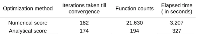
For numerical optimization, the BFGS method (named after Broyden, Fletcher, Goldfer and Shanno) is used in this paper. The BFGS routine is one of the better optimization routines for non-linear optimization, which does not require an analytical Hessian as an input (Nocedal and Wright, 1999). It employs finite-difference approximation for the score, and the only input required in the optimization is the objective function. But having an analytical score in the optimization will lead to an increase in the accuracy of estimates and a faster speed of convergence. Unfortunately, no analytical score for CCC-MGARCH or DCC-MGARCH model has been provided in the literature.6 For this reason, the analytical score for the LMGARCH model has to be derived and the result is provided in Appendix A. For the CCC case, through observation in the application to both simulated and real data, the use of the analytical score in the optimization significantly reduces the time for convergence and also increases accuracy. Table 2 provides an example illustrating how the analytical score increases the speed of convergence. In the example, the unrestricted CCC-MGARCH(1,1) model with twelve dimensions (or an unbanded CCC-LMGARCH(1,1) model) is used. The number of observations of the data is 719. The number of iterations taken till convergence, the total number of times that the objective function is evaluated and the elapsed time are recorded. As can be seen, the analytical score over-performs the numerical score by reducing all three measures significantly. In particular, the elapsed time has been reduced by approximately 90% when using the analytical score.
Optimization method Iterations taken till
convergence Function counts
Elapsed time ( in seconds)
Numerical score 182 21,630 3,207
Analytical score 174 194 327
Table 2: Speed of convergence comparison under optimization using numerical and analytical scores for estimating an CCC-MGARCH(1,1) model with 12 dimensions
But for the DCC case, due to the non-trivial nature of evaluating the analytical score, the benefit of using the analytical score is much less. See Appendix A for the derivation on the analytical score for the CCC-LMGARCH model and a discussion for the DCC case.
6
5
Application to Simulated Data
In order to demonstrate the model and evaluating the reliability of the estimation method discussed in the previous chapters, a small simulation based on a band-one LMGARCH model with six dimensions is discussed here. Two sets of simulated data are generated: one from a band-one CCC-LMGARCH model and the other from a band-one DCC-LMGARCH model.
5.1 Estimation of the Simulated Data from a CCC-LMGARCH
Model
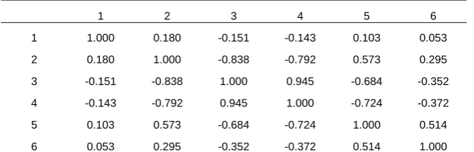
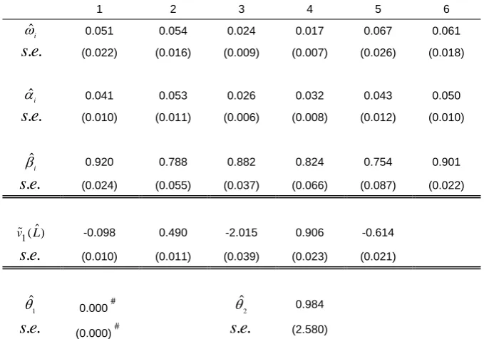
A sample of 3000 observations with 6 dimensions is generated from the band-one CCC-LMGARCH model using the true parameter values listed in Table 3. Parameters in the constant correlation matrix C are determined by the parameters in the lower triangular matrixL in (4.7). The true constant correlation matrix resulting from the specification of L is provided in Table 4. Estimation has been conducted through three different models: univariate GARCH on each equation, CCC-LMGARCH, and DCC-LMGARCH, although CCC-LMGARCH is the true model from which the data was generated.
3000
n 1 2 3 4 5 6
i
0.07 0.05 0.03 0.02 0.04 0.06
i
0.05 0.05 0.03 0.03 0.03 0.05
i
0.90 0.80 0.85 0.80 0.85 0.90
1( )
v L -0.1 0.5 -2.0 0.9 -0.6
Table 3: True parameter values used in simulating data through a band-one CCC-LMGARCH model
1 2 3 4 5 6
1 1.000 0.180 -0.151 -0.143 0.103 0.053
2 0.180 1.000 -0.838 -0.792 0.573 0.295
3 -0.151 -0.838 1.000 0.945 -0.684 -0.352
4 -0.143 -0.792 0.945 1.000 -0.724 -0.372
5 0.103 0.573 -0.684 -0.724 1.000 0.514
6 0.053 0.295 -0.352 -0.372 0.514 1.000
Table 4: The true correlation matrix resulting from the parameters specified for matrix L . In the CCC-LMGARCH case, this is the constant correlation matrix C in (4.7). In the DCC-LMGARCH case, this is the marginal correlation matrix
1 1
2 2
A. Univariate GARCH
1 2 3 4 5 6
ˆi
0.052 0.102 0.078 0.073 0.140 0.056
. .
s e (0.020) (0.037) (0.078) (0.040) (0.062) (0.021)
ˆi
0.042 0.072 0.025 0.047 0.060 0.047
. .
s e (0.010) (0.018) (0.018) (0.022) (0.022) (0.011)
ˆ
i
0.919 0.627 0.668 0.351 0.517 0.908
. .
s e (0.021) (0.118) (0.314) (0.344) (0.197) (0.025)
B. CCC-LMGARCH
1 2 3 4 5 6
ˆi
0.052 0.054 0.024 0.017 0.067 0.061
. .
s e (0.022) (0.016) (0.008) (0.007) (0.026) (0.018)
ˆi
0.041 0.053 0.026 0.032 0.043 0.050
. .
s e (0.010) (0.011) (0.006) (0.008) (0.012) (0.010)
ˆ
i
0.920 0.788 0.882 0.824 0.754 0.901
. .
s e (0.024) (0.054) (0.035) (0.062) (0.086) (0.022)
1( )ˆ
v L -0.098 0.490 -2.015 0.906 -0.614
. .
s e (0.010) (0.011) (0.039) (0.023) (0.021)
C. DCC-LMGARCH
1 2 3 4 5 6
ˆi
0.051 0.054 0.024 0.017 0.067 0.061
. .
s e (0.022) (0.016) (0.009) (0.007) (0.026) (0.018)
ˆi
0.041 0.053 0.026 0.032 0.043 0.050
. .
s e (0.010) (0.011) (0.006) (0.008) (0.012) (0.010)
ˆ
i
0.920 0.788 0.882 0.824 0.754 0.901
. .
s e (0.024) (0.055) (0.037) (0.066) (0.087) (0.022)
1( )ˆ
v L -0.098 0.490 -2.015 0.906 -0.614
. .
s e (0.010) (0.011) (0.039) (0.023) (0.021)
1
ˆ
0.000# 2
ˆ
0.984
. .
s e (0.000)# s e. . (2.580)
Table 5: ML estimates for the simulated data from band-one CCC-LMGARCH DGP through three different models. (A) Separate univariate GARCH models on each equation; (B) CCC-LMGARCH model with band one; (C) DCC-CCC-LMGARCH model with band one. # These numbers are not exactly zeros, but are of order 11
The initial conditions for the GARCH coefficients i, i and i are set to be 0.5, 0.5 and 0.4 respectively uniformly across all 'i s, which are values moderately different from the true values. Separate univariate GARCH models on each equation are firstly estimated. Then the estimates from these univariate GARCH models are taken as initial conditions for the corresponding GARCH coefficients in the CCC and DCC LMGARCH models. The initial conditions of the elements on the first lower diagonal band of L, or v L1( ), in the LMGARCH model are set in the following way: The fitted standardized innovations ˆt are firstly obtained from estimating the univariate GARCH models on each equation; Then the sample covariance matrix Cof these standardized innovations ˆt is calculated as ( T1 ˆ ˆ') /
t t t
C
T ; Finally, the elements on the first lower diagonal band of the inverse of this sample covariance matrix, namely v C1( 1), are used as initial conditions for v L1( ) . For 1 and 2 in the DCC case, initial conditions are set to 0.4 and 0.4, respectively. These values are moderately different from the true parameter values, which could be the case in real applications when only some indication of the true parameters exists.5.2 Estimation of the Simulated Data from a DCC-LMGARCH
Model
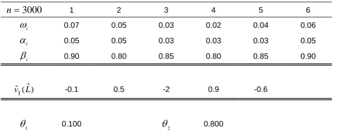
Similar to the previous case, another sample of 3000 observations with 6 dimensions is generated from a band-one DCC-LMGARCH model. The true parameters are listed in Table 6. They are the same as in section 5.1 except that the true values of the extra parameters 1 and 2 are now 0.10 and 0.80, respectively. The resulting marginal correlation matrix, as opposed to the constant correlation matrix as before, is in Table 4.
3000
n 1 2 3 4 5 6
i
0.07 0.05 0.03 0.02 0.04 0.06
i
0.05 0.05 0.03 0.03 0.03 0.05
i
0.90 0.80 0.85 0.80 0.85 0.90
1( )ˆ
v L -0.1 0.5 -2 0.9 -0.6
1
0.100
2
0.800
Table 6: True parameter values used in simulating data through a band-one DCC-LMGARCH model
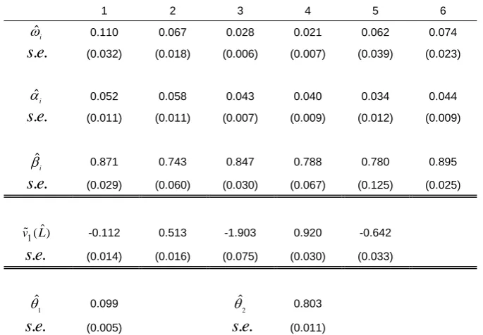
Estimation using the same three models is conducted and all initial conditions are set in a similar way in the last section. Table 7 shows the results of estimation, which are different across the models. The correct inclusion of a dynamic structure in the DCC-LMGARCH results in estimates that are much closer to the true values than that of the other two models. There are two estimates (indicated by stars) of the CCC-LMGARCH model are statistically significantly different from the true values of the corresponding parameters at 5% level by using the asymptotic normal test. This suggests that, when the conditional correlation matrix is in fact time-varying, ignoring this dynamic structure may lead to biased estimates. The estimates of 1 and 2 in the DCC-MGARCH model is very close to the true values with very small standard errors. The standard errors of the GARCH coefficient estimates from using the DCC-LMGARCH model are also noticeably smaller. All these show the advantage in using the DCC-LMGARCH model, when the conditional correlation matrix of the data follows a dynamic structure, which could be the case for intraday financial time series. In the following two chapters, the LMGARCH model will be applied to two sets of real data.
A. Univariate GARCH
ˆi
0.123 0.051 0.026 0.018 0.032 0.051
. .
s e (0.041) (0.022) (0.013) (0.010) (0.017) (0.026)
ˆi
0.062 0.046 0.043 0.043 0.033 0.031
. .
s e (0.014) (0.013) (0.014) (0.017) (0.012) (0.010)
ˆ
i
0.854 0.803 0.854 0.806 0.872 0.925
. .
s e (0.038) (0.074) (0.062) (0.094) (0.059) (0.030)
B. CCC-LMGARCH
1 2 3 4 5 6
ˆi
0.127 0.057 0.027 0.026 0.095 0.050
. .
s e (0.038) (0.020) (0.008) (0.009) (0.151) (0.021)
ˆi
0.061 0.042 0.032 0.036 0.015 0.025*
. .
s e (0.013) (0.011) (0.007) (0.009) (0.015) (0.008)
ˆ
i
0.852 0.786 0.860 0.748 0.700 0.931
. .
s e (0.034) (0.066) (0.036) (0.082) (0.463) (0.023)
1( )ˆ
v L -0.111 0.631* -1.419 0.913 -0.606
. .
s e (0.011) (0.014) (0.029) (0.023) (0.021)
C. DCC-LMGARCH
1 2 3 4 5 6
ˆi
0.110 0.067 0.028 0.021 0.062 0.074
. .
s e (0.032) (0.018) (0.006) (0.007) (0.039) (0.023)
ˆi
0.052 0.058 0.043 0.040 0.034 0.044
. .
s e (0.011) (0.011) (0.007) (0.009) (0.012) (0.009)
ˆ
i
0.871 0.743 0.847 0.788 0.780 0.895
. .
s e (0.029) (0.060) (0.030) (0.067) (0.125) (0.025)
1( )ˆ
v L -0.112 0.513 -1.903 0.920 -0.642
. .
s e (0.014) (0.016) (0.075) (0.030) (0.033)
1
ˆ
0.099
2
ˆ
0.803
. .
s e (0.005) s e. . (0.011)
6
Application of the CCC-LMGARCH Model to
BHP Intraday Stock Returns
In this chapter, the CCC-LMGARCH model will be fitted to BHP intraday stock returns. The reason that the CCC-LMGARCH model is used rather than the more general DCC-LMGARCH model is because the hypothesis of constant correlation, namely that 1 and 2 are jointly zeros, cannot be rejected under the LR test, which can be easily conducted due to the aforementioned nested nature of the CCC-LMGARCH and DCC-LMGARCH models.
6.1 A Brief Review of the Literature
Since its introduction, the univariate GARCH has been used extensively in analysing time-varying conditional volatility for financial data at low frequencies (Month, weekly, daily). Unfortunately, the mean and volatility of stock returns do not follow the same processes at each point in time over any given day. Wood et al. (1985) used one-minute returns of NYSE stocks to show that there is a diurnal pattern of returns and volatility during a trading day, with returns and volatility both being higher in the beginning and the end of the day than in the middle of the day. This pattern looks like a “U” (or more precisely a flipped “J”) if the returns and volatility are plotted against time of day. Harris (1986) also found a similar diurnal pattern in volatility using 5-minute market index data for the US. The high volatility at the opening phase of the market is generally caused by rapid price adjustment resulting from the information flow that has occurred overnight. The distinctly different magnitude of volatility over a trading day implies that fitting a GARCH model, either univariate or multivariate, on daily data while ignoring the intraday pattern of volatility may lead to erroneous conclusions.
volatility of stock returns, the GARCH process obtained from using daily returns should be consistent with the GARCH process obtained from temporally aggregating of the higher frequency GARCH processes, say 30-minute returns. Although results of temporal aggregation of MGARCH have not been fully developed (Hafner, 2004, and Hafner and Rombouts, 2006), many studies on temporal aggregation of the univariate GARCH model have found the theoretical result is rejected by empirical data with high frequency (Dacorogna et al., 2001 and Guillaume et al., 1995). This rejection suggests that volatility is heteroskedastic at each period in a day, and the assumption that there is only one underlying GARCH model across a day is not appropriate. This is strong motivation for using a longitudinal structure. Andersen and Bollerslev (1997) concluded, based on their studies on periodicity of intraday volatility, that results from modelling interday volatility while ignoring the strong intraday periodicity are likely to be biased and erroneous. The LMGARCH model, which fits univariate GARCH processes on data at different times of day, can account for this intradaily periodicity and thus justifies its use on high frequency longitudinal data.
In the finance literature, the financial markets, especially for highly-liquid stocks like BHP, are assumed to be at least weak-form efficient. This implies that returns are not correlated over time, which is usually observed to be true for low frequency data (monthly, weekly, daily data). However, for high frequency data, correlation of returns over short periods of time may be observed and is often negative for stock returns. This correlation tends to disappear as the frequency becomes lower. One of the most popular explanations of this observation is that the correlation is spurious and is created by market microstructure, such as bid-ask bounces (Roll, 1984), nonsynchronous trading (Lo and MacKinlay, 1990) or simply recording errors in the data, though some recent evidence shows that partial price adjustment may be the main reason for the significant correlation between high frequency returns (Andersen et al., 2005). The CCC-LMGARCH model is able to capture this significant correlation over time of day through the constant correlation matrix C. See Boudoukh et al. (1994) for a more detailed discussion on the autocorrelations of short-horizon stock returns.
6.2 Data
compounded intraday returns of trading days between 3-July-2002 and 4-May-2005 are analysed. Returns at two frequencies are calculated and aggregated from the trade-by-trade prices of BHP stock. These are 30-minute and 5-minute returns between 10:00 am and 4:00pm of each trading day. The first return for each day (10:30 for the 30-minute case and 10:05pm for the 5-minute case) is calculated by using the last traded price at the end of that first interval and the closing price of the last trading day. This means that the overnight return is included in the first return of each day. Observations are available for 719 days, with the cross-sectional dimension of the data being 12 for the 30-minute returns and 72 for the 5-minute returns. However, due to unreliability of the returns between 3:55pm and 4:00pm, the return during the last five minutes of trading day is discarded, leaving only 71 intraday returns for the 5-minute data. All 30-minute trading intervals have trades occurring during the period and only around 1% of the 5-minute trading intervals have no trade during the interval. This reflects the fact that BHP is actively traded on the market and the non-synchronous trading effect is therefore expected to be weak. All returns have been mean-corrected for a constant level before running a CCC-LMGARCH model. The dataset was used by Brassil (2005) with 30-minute intervals for a longitudinally parsimonious multivariate stochastic volatility model.
6.3 Estimation Results
6.3.1 Results for the 30-minute Data
This section shows the results of fitting the 30-minute data by CCC-LMGARCH model. Since the dimension of the model is 12, results of models at all bandwidths from 0 to 11 have been provided below for comparison.
Model Bandwidth
on Precision
Matrix C1
Log
likelihood
value
Number of
parameters
Likelihood
ratio AIC SIC
Generalized
Variance of
ˆ
C
Average
Generalized
Variance of Hˆt (1062)
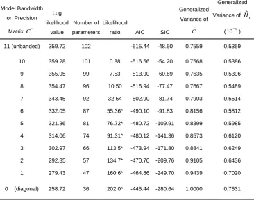
11 (unbanded) 359.72 102 -515.44 -48.50 0.7559 0.5359
10 359.28 101 0.88 -516.56 -54.20 0.7568 0.5386
9 355.95 99 7.53 -513.90 -60.69 0.7635 0.5396
8 354.47 96 10.50 -516.94 -77.47 0.7667 0.5489
7 343.45 92 32.54 -502.90 -81.74 0.7903 0.5514
6 332.05 87 55.36* -490.10 -91.83 0.8156 0.5812
5 321.36 81 76.72* -480.72 -109.91 0.8399 0.5985
4 314.06 74 91.31* -480.12 -141.36 0.8573 0.6120
3 302.97 66 113.5* -473.94 -171.80 0.8841 0.6249
2 292.35 57 134.7* -470.70 -209.76 0.9105 0.6436
1 279.43 47 160.6* -464.86 -249.70 0.9439 0.7020
0 (diagonal) 258.72 36 202.0* -445.44 -280.64 1.0000 0.7531
Table 8: Comparison of models of 30-minute BHP stock returns at different bandwidth on precision matrix. Likelihood ratio is used to test for model against the null hypothesis that the corresponding band structure of the precision matrix is true. Numbers indicated by stars means they are statistically significant at 5% level.
Time of
day 10:30 11:00 11:30 12:00 12:30 13:00 13:30 14:00 14:30 15:00 15:30 16:00
ˆi (10 )5
0.2743 0.0707 0.0701 0.0282 0.0137 0.0013 0.0032 0.0210 0.0060 0.0053 0.1052 0.0345
. .
s e (0.1683) (0.0503) (0.0515) (0.0139) (0.0096) (0.0010) (0.0044) (0.0084) (0.0041) (0.0039) (0.0665) (0.0225)
ˆi
0.0400 0.0398 0.0530 0.0583 0.0582 0.0166 0.0142 0.0670 0.0298 0.0307 0.0716 0.0897
. .
s e (0.0137) (0.0221) (0.0278) (0.0226) (0.0267) (0.0066) (0.0107) (0.0229) (0.0108) (0.0121) (0.0365) (0.0353)
ˆ
i
0.9419 0.8629 0.8270 0.8822 0.9069 0.9764 0.9685 0.8509 0.9597 0.9587 0.7535 0.8601
. .
s e (0.0191) (0.0833) (0.1032) (0.0400) ('0.0458) (0.0080) (0.0319) (0.0480) (0.0144) (0.0164) (0.1370) (0.0599)
ˆ ˆi i
0.9819 0.9026 0.8800 0.9405 0.9651 0.9929 0.9827 0.9179 0.9895 0.9893 0.8251 0.9497
MSD 3.8963 0.8519 0.7644 0.6887 0.6274 0.4298 0.4288 0.5062 0.7600 0.7062 0.7758 0.8290
In Table 8, the null hypothesis of the LR test is that the corresponding band structure is true, with the alternative being the unbanded model. The LR test suggests the band structure imposed on the precision matrix C1 is rejected at the 5% level for a bandwidth of 6 or lower. Table 8 also includes two information criteria, the Akaike information criterion (AIC) and the Schwarz information criterion (SIC), for models at each bandwidth. The formula for the AIC and the SIC are as follows:
2 ( ) 2
AIC l p (6.1)
2 ( ) ln( )
SIC l p T (6.2)
Here, l( ) is the log-likelihood value, pis the number of parameters in the model and
T is the number of observations of data (Judge et al., 1985). Given two models, the model with a lower value of information criterion is the one to be preferred. In Table 8, the two information criteria are pointing in different directions: AIC suggests using a model with a bandwidth of 8, while SIC, which tends to favour more parsimonious models, suggests that the band zero model should be used. However, it would be inappropriate to follow the SIC and to assume that there is no correlation at all between time of day, since the LR ratios are significant at low bandwidths. However, although the band structures with bandwidth 6 or lower are rejected, models with bandwidth one or two successfully capture most of the variation of the data as according to the small decrease in the AIC as the bandwidth increases.
In addition to the information criteria, measures of the goodness of fit of the correlation and covariance matrices are also provided in Table 8. Generalized variance of a matrix is the determinant of the matrix, which is a measure of the spread of the matrix. (Anderson, 1984) Average generalized variance, 1
ˆ
( T ) /
t t H T
is calculated for ˆt H
A. Correlation coefficient estimates
Time of day 10:30 11:00 11:30 12:00 12:30 13:00 13:30 14:00 14:30 15:00 15:30 16:00
1 1.000
2 0.004 1.000
3 0.094* 0.063 1.000
4 0.085* 0.031 0.039 1.000
5 0.008 0.031 0.024 -0.063 1.000
6 0.019 0.083* 0.062 0.082* -0.010 1.000
7 0.096* 0.035 0.109* 0.053 -0.008 -0.009 1.000
8 0.123* 0.076* 0.081* -0.002 0.001 -0.041 -0.188* 1.000
9 0.118* 0.039 0.107* 0.054 0.022 0.069 0.085* 0.069 1.000
10 -0.013 -0.049 0.051 0.013 -0.021 -0.043 0.005 -0.081* -0.083* 1.000
11 0.030* 0.022* 0.125* 0.087* 0.054 0.054 0.067 0.039 0.035 -0.024 1.000
12 0.032* 0.019* 0.028 0.105* 0.001 0.073* 0.043 0.076* 0.091* 0.000 0.013 1.000
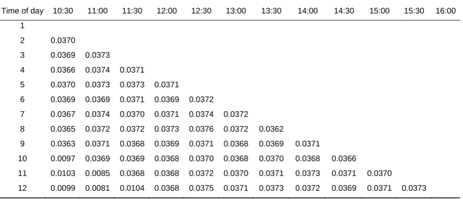
B. Standard errors of correlation coefficient estimates
Time of day 10:30 11:00 11:30 12:00 12:30 13:00 13:30 14:00 14:30 15:00 15:30 16:00
1
2 0.0370
3 0.0369 0.0373
4 0.0366 0.0374 0.0371
5 0.0370 0.0373 0.0373 0.0371
6 0.0369 0.0369 0.0371 0.0369 0.0372
7 0.0367 0.0374 0.0370 0.0371 0.0374 0.0372
8 0.0365 0.0372 0.0372 0.0373 0.0376 0.0372 0.0362
9 0.0363 0.0371 0.0368 0.0369 0.0371 0.0368 0.0369 0.0371
10 0.0097 0.0369 0.0369 0.0368 0.0370 0.0368 0.0370 0.0368 0.0366
11 0.0103 0.0085 0.0368 0.0368 0.0372 0.0370 0.0371 0.0373 0.0371 0.0370
12 0.0099 0.0081 0.0104 0.0368 0.0375 0.0371 0.0373 0.0372 0.0369 0.0371 0.0373
Table 10: Correlation coefficient estimates of CCC-LMGARCH on 30-minute BHP intraday returns between different times of day. Starred numbers are statistically significant at the 5% level.
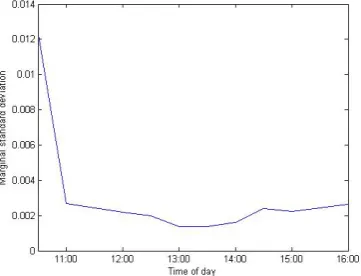
Table 9 shows the GARCH coefficient estimates for the CCC-LMGARCH model with bandwidth eight. Standard errors are calculated using the Delta method with a numerical Hessian matrix. Through comparison (results not shown), it was found that the GARCH equation coefficient estimates are not very sensitive to the bandwidth choice. One should notice that, due to the non-linear nature of the GARCH model, 's and 's are not directly comparable between different time periods, but what can be compared is (Andersen and Bollerslev, 1997). So the sum of and , which is a measure of the persistence level, together with the marginal standard deviation,
/(1 )
i i i
marginal standard deviation plotted in Figure 1 exhibits a flipped “J”, which confirms our expectations of intraday dependency of the parameters in the GARCH model. The volatility in the beginning of the day is the highest and volatility is the lowest during lunch time and then gradually rises again towards the end of the day. The highest volatility is approximately five to six times larger than the lowest, which are magnitudes comparable to previous empirical studies like Wood et al. (1985) when overnight returns are included in the first returns of each trading day. This intraday periodicity indicates the existence of heteroskedasticity in volatility as mentioned before, which demonstrates the benefits of using a LMGARCH model on the longitudinal data.
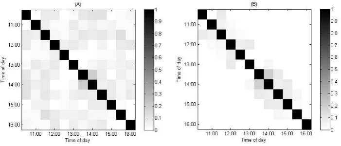
Table 10 provides the estimated correlation matrix ( ˆC) and their standard errors at band 8, where Cˆ [diag( )]ˆ 12ˆ[diag( )]ˆ 12 and ˆ (LLˆ ˆ')1.It is confirmed by the
Figure 2: (A) Image of absolute value of Cˆ from fitting a band-eight CCC-LMGARCH model on BHP 30-minute returns; (B) Image of absolute value of Cˆ from fitting a band-two CCC-LMGARCH model on BHP 30-minute returns; Elements in Cˆ are correlation coefficients.
6.3.2 Results for the 5-minute Data
Figure 3: Plot of the marginal standard deviation implied by the estimated CCC-LMGARCH coefficients at bandwidth two for BHP 5-minute returns. A diurnal pattern can be observed in the diagram.
Figure 4: (A) Image of the absolute value of the elements in Cˆ estimated by fitting a band-two CCC-LMGARCH model on BHP 5-minute returns. The elements in Cˆ are correlation coefficients. (B) A zooming-in image on the lunch time section of image (A) .
panel D says that the correlation between 13:00 and 13:20 (5 4 minute interval) is very close to zero. The interesting point from Figure 5 is not only that the correlations are negative at band one during the middle of the day, but also that they are more negative than they were in the 30-minute data. While the most negative correlation is -0.188 in Table 10, the most negative correlation for the 5-minute data is -0.370, nearly twice as large as before. The more significant negative correlation in higher frequency data is also well documented in the literature, with bid-ask bounce and non-synchronous trading effects being more notable over shorter time (see Dacorogna et al. for example). As can be seen from panel A to D, the correlation becomes weaker and weaker as the time interval becomes longer and the market microstructure effects become less significant.
7
Application of the DCC-LMGARCH Model to
Intraday Electricity Log Prices
In the last chapter, some interesting and significant intraday patterns for stock returns were uncovered using a CCC-LMGARCH model. However, the constant correlation hypothesis cannot be rejected in the BHP returns. The electricity data used in this chapter, on the other hand, is found to follow a dynamic conditional correlation structure, based on an LR test on 1 and 2 in (3.3). Previous research on electricity
spot prices has not accounted for the very pronounced intraday heteroskedasticity in the data. (See Bunn and Karakatsani (2003), Escribano et al. (2002), and Knittel and Roberts (2005) for more discussion.) Understanding the volatility and correlation dynamics of intraday electricity spot prices is important to traders because their exposure to the spot usually varies through the day. Cottet and Smith (2003) firstly used a parsimonious banded model on the longitudinal intraday electricity demand data, which takes into account the intraday heteroskedasticity. Smith and Cottet (2006) apply the idea to model intraday electricity prices using a stochastic volatility framework. All of these studies, however, are carried out in a Baysian framework.
7.1 A Brief Overview
Over the last decade, wholesale electricity markets have been introduced in many developed countries. In Australia, the Australian National Electricity Market (NEM) has been in operation since 1998. This national market connects the previously state-based electricity market and is currently supplying electricity to approximately 8 million customers across Queensland, New South Wales (NSW), Victoria, South Australia and the Australian Capital Territory. (Smith and Cottet, 2006) It is the wholesale spot prices of electricity in this market that are used for modelling in this chapter.
forecast then dispatch capacity according to the bid-price order. So, generators with lower marginal costs will generate capacity first at lower prices. As the demand is gradually matched by generators, available capacity from low-marginal cost generators decreases and the unmatched demand must be generated at higher marginal costs and bid prices rise accordingly. The equilibrium price is then determined by the highest bid-price of the last unit of electricity generated to match the demand. This bid-bid-price process mimics the very price determination mechanism in a more conventional free market. Thus, demand and supply are strong systemic components in determining the electricity spot price. In general, the higher the short-term demand, the higher the spot price is. However, since marginal cost increases in a non-linear fashion as demand rises and usually increases rapidly when there is a sudden increase in demand, the demand affects prices positively at an increasing rate. On the supply side, data is much more difficult to obtain due to possible rebidding and the market sensitivity of the data. Nevertheless, missing supply side factors may result in both intra- and inter- day autocorrelation, which can be captured by the using of the DCC-LMGARCH model in this paper. For a more detailed discussion about the NEM and price determination, see Smith and Cottet (2006) and references therein.
7.2 Data
In this chapter, log hourly spot prices of electricity in New South Wales (NSW), between 14-Dec-1998 and 31-Dec-2000 are examined. Log prices, rather than returns, are used in this application due to the non-storable nature of electricity. Electricity is a flow commodity and is almost impossible to store in the absence of a sizeable hydroelectric generation capacity, which means arbitrage over time is no possible. Thus it is more meaningful to use log spot prices, which reflect a series of equilibriums of demand and supply, as a time series here.
4 3
0 1 , 1 ,1 6 ,6
1 1
log it i i log i t i j ijt i it i m imt it,
j m
p p X D S a
(7.1):
log is the log spot price for the th hour at day
1, 2, 3, 4, are day type dummies for the th hour observation at day .
, is the scaled demand lying in the unit interval for the
it ijt it
where
p i t
X for j i t
D
th hour observation at day . 1, 2, 3 are the spline terms to capture the non-linearity between price and demand.
imt
i t
S for m
The day dummies indicate on which day the observation is taken. X1 1, if it is on a Monday, X2 1, if it is on a Friday, X3 1, if it is on a Saturday and X4 1, if it is on a Sunday or a public holiday. So, the intercept i0 is the base case indicating a day between Tuesday and Thursday. These dummies capture the inter-daily level of the log price of electricity. Demand for electricity is included in the regression in a scaled form:
[ min( )] / ( )
it it i i
D demand demand range demand . So demand has been scaled to be within the unit interval. Three basis terms Simt
Dit Km
2log
Dit Km
, where,0.3, 0.6 m
K and 0.9 are included to capture the potential non-linearity between log price and demand. In essence, regression (7.1) is used for filtering out the systemic component of log spot prices. The innovations ˆat resulting from OLS of (7.1) will be used as the longi