Finite Difference Solution of Mixed Convective Heat Transfer Transient Flow along a Continuously Moving Cooled Plate

Annals of Pure and Applied Mathematics Vol. 7, No. 2, 2014,18-26

ISSN: 2279-087X (P), 2279-0888(online) Published on 27 August 2014

www.researchmathsci.org

18

Annals of

Finite Difference Solution of Mixed Convective Heat

Transfer Transient Flow along a Continuously Moving

Cooled Plate

U. Sarder, M. M. Haque* and T. Ferdaus

Mathematics Discipline

Khulna University, Khulna-9208, Bangladesh *

Corresponding author’s E-mail: [email protected]

Received 1 August 2014; accepted 26 August 2014

Abstract. Numerical study of a mixed convective heat transfer transitory flow of a

viscous incompressible fluid along a continuously moving semi-infinite vertical cooled plate is completed here. It is also assumed that the plate is embedded in a porous medium. This investigation is performed for cooling problem with the both air and water. A mathematical model related to the problem is developed from the basis of studying Fluid Dynamics(FD). To solve the problem, an explicit procedure of finite difference method with stability and convergence criterion has been used in this work. Both the local and average shear stress with Nusselt number is also computed here. The obtained numerical values of velocity, temperature, shear stress and Nusselt number are plotted in graphs for different values of associated parameters as well as the physical aspects of the problem are discussed in details. Finally, some important findings are concluded here.

Keywords: Transient Flow, Heat Transfer, Mixed Convective, Finite Difference

AMS Mathematics Subject Classification (2010): 58D30, 35Q35

1. Introduction

The heat transfer flow of an electrically conducting viscous fluid is considered to be of significant importance due to its application in many engineering problems such as nuclear reactors and those dealing with liquid metals. The convective heat transfer problems play a decisive role in geothermal energy recovery, oil extraction, thermal energy storage and flow through filtering devices. Finston [1] studied a natural convective heat transfer flow of fluid. A similar solution for laminar free convection from a non-isothermal vertical plate was computed by Sparrow and Gregg [2]. A general series solution of free convective heat transfer flow from a non-isothermal vertical flat plate has been obtained by Kuiken [3]. Quit recently, a numerical study is performed for a free convective heat transfer flow of a viscous fluid by Fadzilah et al. [4].

19

convection flow through a porous medium. Raptis et al. [5] have observed the steady free convective flow through a porous medium bounded by an infinite surface by use of the model of Yamamoto and Iwamura [6] for the flow near the surface. Three dimensional free convective heat transfer flow through a porous medium has been studied by Ahmed and Sarma [7]. Chaudhury and Chand [8] further investigated the same problem. Recently, the analytic solutions for unsteady free convection in porous media have been obtained by Magyari et al. [9].

All the above works are related to the stationary vertical plate. However, the flow past a continuously moving plate has many applications in manufacturing processes such as hot rolling, metal and plastic extrusion, continuous casting, glass fiber and paper production. Sakiadis [10] was the first author to recognize this backward boundary layer situation and used a similarity transformation to obtain a numerical solution for the flow field of a continuously moving plate. The steady heat transfer flow past a continuous moving plate with variable temperature was analyzed by Soundalgekar and Ramana Murty [11]. A solution of mixed convective heat transfer flow along a continuously moving heated vertical plate with suction or injection has been computed by Sami and Al-Sanea [12].

The mixed convective fluid flows play an important role in a number of industrial applications such as fiber and granular insulation, geothermal systems etc. Hence, our main aim is to investigate a mixed convective heat transfer unsteady flow along a continuously moving plate surrounded by a porous medium.

2. Mathematical model of flow

A time dependent mixed convective heat transfer flow of an electrically conducting viscous incompressible fluid past an electrically non-conducting semi-infinite vertical cooled plate embedded in a porous medium is considered here. The flow is also assumed to be in the x-direction which is taken along the plate in the upward direction and y -axis is normal to it. Initially, we consider that the plate as well as the fluid particles are at rest at the same temperature T =T_∞ at all points, where T_∞ be the fluid temperature of uniform flow. It is assumed that the plate be at rest after that the plate is to be moving with a constant velocity U0 in its own plane.

Within the framework of the above stated assumptions, the equations relevant to the present problem are governed by the following system of coupled non-linear partial differential equations,

Continuity Equation =0

∂ ∂ + ∂ ∂

y v x u

Momentum Equation

(

)

u

K y

u T

T g y u v x u u t u

′ − ∂ ∂ + − =

∂ ∂ + ∂ ∂ + ∂

∂

_β

_υ

υ

α 2

2

Energy Equation

2

2 2

     

∂ ∂ + ∂ ∂ = ∂ ∂ + ∂ ∂ + ∂ ∂

y u c y

T c y T v x T u t T

p p

υ

ρ

20

The corresponding initial and boundary conditions are given below,

∞ = =

=

= u v T T

t 0, 0 0 everywhere

∞ = =

=

> u v T T

t 0, 0 0 at x=0 u=U₀ v=0 T =T_w at y=0 u=0 v=0 T =T_∞ as y→ ∞

where x and y be the Cartesian coordinates, u & v are velocity components, t denotes time, g is the local acceleration due to gravity,

β

is thermal expansion coefficient,

υ

is kinematic viscosity,

ρ

is density, K′ is the permeability of the porous medium,

κ

is thermal conductivity, c_p is specific heat at constant pressure and T_w be the fluid temperature near at plate.

3. Mathematical formulation

To find the solution of the problem, it is required to transfer the system of equations into a non-dimensional system, so we take the following dimensionless quantities,

υ

τ

υ

υ

2 0 0 0 0 0 , , , , tU U v V U u U yU Y xU

X = = = = = and

w T T T T T ∞ ∞ − = −

where

τ

represents the dimensionless time, X & Y be the dimensionless cartesian

coordinates, U and V be the dimensionless velocity components and T be the dimensionless temperature.

Using the above relations, we obtain the following non-dimensional coupled partial differential equations, 0 = ∂ ∂ + ∂ ∂ Y V X U U K Y U T G Y U V X U U U r 1 2 2 − ∂ ∂ + = ∂ ∂ + ∂ ∂ + ∂ ∂

τ

2 2 2 1 c r

T T T T U

U V E

X Y P Y Y

τ

∂ ∂ ∂ ∂ ∂ 

+ + = +  

∂ ∂ ∂ ∂ ∂ 

where

(

₃

)

0 U

T T g

Gr w

∞ −

=

υ

β

(Grashof Number),

κ

υρ

p

r c

P = (Prandtl Number)

2 3 0

υ

K U

K = ′ (Permeability Number) and

(

− ∞

)

= T T c U E w p c 2 0 (Eckert Number).

Also the associated initial and boundary conditions become 0 , 0 , 0 ,

0 = = =

= U V T

τ

everywhere

0 , 0 , 0 ,

0 = = =

> U V T

τ

at X =0

21 4. Shear stress and nusselt number

Since the quantities of chief physical interest are shear stress and Nusselt number, hence from the velocity field, we study the effects of various parameters on the local and average shear stress. The following equations represent the local and average shear stress at the plate.

Local shear stress,

0 L Y U Y

τ

µ

= ∂   = _∂ 

  and average shear stress, 0 A Y U dX Y

τ

µ

= ∂   = _∂   

∫

which are proportional to

0 =       ∂ ∂ Y Y U

and

∫

=       ∂ ∂ 100 0 0 dX Y U Y respectively.

And from the temperature field, we investigate the effects of various parameters on the local and average heat transfer coefficients. The following equations represent the local and average heat transfer rate that is well known Nusselt number.

Local Nusselt number,

0 uL Y T N Y

µ

=  _∂  = −_∂ 

  and

Average Nusselt number,

0 uA Y T N dX Y

µ

=  _∂  = −_∂   

∫

which are proportional to

0 Y T Y ₌  _∂  −  _∂ 

  and

∫

 ₌     ∂ ∂ − 100 0 0 dX Y T Y respectively.

5. Numerical solution

The explicit finite difference method has been used to solve the governed second order nonlinear coupled dimensionless partial differential equations with the corresponding initial and boundary conditions. To obtain a system of finite difference equations, the flow region is divided into a grid or meshes of lines parallel to X and Y axes where X-axis is taken along the plate and Y-X-axis is normal to the plate. Here it is considered that

(

100

)

max =

X i.e. X varies from 0 to 100 and regard Ymax

(

=25

)

as corresponding to ∞

→

Y i.e. Y varies from 0 to 25. It is also considered that m=100 and n=100 grid spacing in the X and Y directions respectively. We have the constant mesh size along X direction, ∆ =X 1.0 0

(

≤ ≤X 100

)

and the constant mesh size along Y direction,

(

)

0.25 0 25

Y Y

∆ = ≤ ≤ with the smaller time-step ∆

τ

=0.01.

Let U′, V′ and T′ denote the values of U , V and T at the end of a time-step respectively. Using the finite difference approximations, we obtain the following appropriate set of finite difference equations,

, 1, , , 1

0

i j i j i j i j

U U V V

X Y

− −

− −

+ =

22 j i r j i j i j i j i j i j i j i j i T G Y U U V X U U U U U , , 1 , , , 1 , , , , ′ = ∆ − + ∆ − + ∆ − ′ _{− +}

τ

( )

ij

j i j i j i U K Y U U U , 2 1 , , 1

, 2 1 _′

− ∆ + − + + −

( )

, , , 1, , 1 , , 1 , , 1

, , 2

2 1

i j i j i j i j i j i j i j i j i j

i j i j

r

T T T T T T T T T

U V

X Y P Y

τ

− + + − ′ − − − − + + + = ∆ ∆ ∆ _∆ 2 , 1 ,       ∆ − + + Y U U

Ec ij i j

and the initial and boundary conditions with the finite difference scheme are, U_{i j}0_, =0, V_{i j,}0 =0, T_{i j,}0 =0

0, 0, 0, 0, 0, 0

n n n

j j j

U = V = T =

,0 1, ,0 0, ,0 1

n n n

i i i

U = V = T =

, 0, , 0, , 0

n n n

i L i L i L

U = V = T = .

Here the subscripts i and j designate the grid points with x and y coordinates respectively and the superscript n represents a value of time,

τ

=n∆

τ

where

... , 2 , 1 , 0 =

n From the initial condition, the values of U and T _{are known at}

τ

=0.

Then at the end of any time-step ∆

τ

, the new temperature T′, the new velocity U′ and V′ at all interior nodal points may be obtained by successive applications of energy and momentum equations respectively. This process is repeated in time and provided the time-step is sufficiently small, hence U , V and T should eventually converge to values which approximate the steady-state solution of the problem. The

stability condition of finite difference method is

( )

2

2

1 r

U V

X Y P Y

τ τ τ

∆ ₊ ∆ ₊ ∆ _≤

∆ ∆ _∆ and the

convergence criteria of the problem is Pr ≥0.32.

6. Results and discussion

23

The values of the Grashof number are taken to be positive

(

G_r >0

)

for the cooling problem and Gr =10.0,11.0and12.0 are considered here. For the most important fluids such as atmospheric air, salt water and water so the results are limited to

71 . 0 = r

P (Prandtl number for air at 20_{C), 1.0}

r

P = (Prandtl number for salt water at 20_{C) and 7.0}

r

P = (Prandtl number for water at 0C

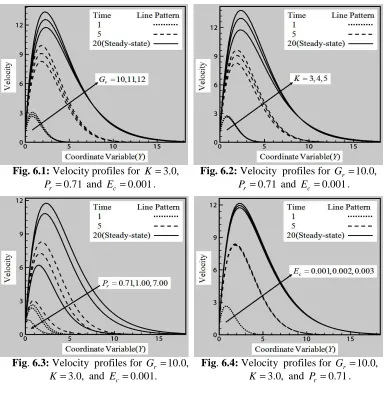
20 ). Also the values of another parameters K and E_c are chosen arbitrarily. The profiles of the transient velocity and temperature versus Y are illustrated in Figs. 6.1-6.8.

The effect of the Grashof number on the velocity field is presented in Fig. 6.1. It is observed that the velocity increases with the rise of G_r. The same effect on the velocity curve is found in Fig. 6.2 that is the velocity increases in case of strong Permeability number. It is observed from Fig. 6.3, the velocity strongly decreases with the increase of Prandtl number. An increasing effect of Eckert number on the velocity profiles are found from Fig. 6.4 at the steady-state.

Fig. 6.1: Velocity profiles for K=3.0, Fig. 6.2: Velocity profiles for G_r =10.0, P_r=0.71 and E_c=0.001. P_r =0.71 and E_c=0.001.

24

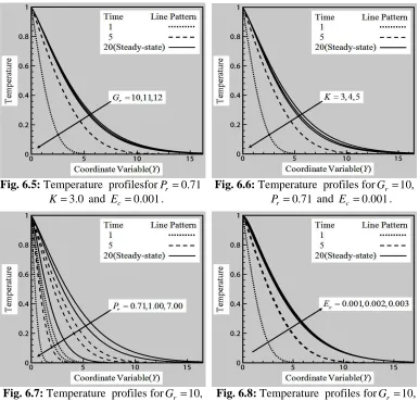
Fig. 6.5 shows that the steady state temperature of fluid decreases in case of strong Grashof number. In Fig.6.6, we see that the fluid temperature decreases for the increasing values of permeability number. A strong decreasing effect of the Prandtl number on the temperature curves are observed from Fig. 6.7. The effect of the Eckert number on the temperature profiles are displayed in Fig. 6.8. It is shown that the temperature increases with the rise of E_c.

Fig. 6.5: Temperature profilesforP_r =0.71 Fig. 6.6: Temperature profiles forG_r =10, K=3.0 and E_c=0.001. P_r =0.71 and E_c=0.001.

Fig. 6.7: Temperature profiles forG_r =10, Fig. 6.8: Temperature profiles forG_r =10, K=3.0 and E_c=0.001. K=3.0 and P_r =0.71.

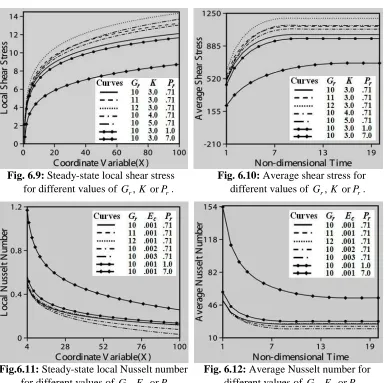
The profiles of steady state local and average shear stress for different values of

, or

r r

25

Fig. 6.9: Steady-state local shear stress Fig. 6.10: Average shear stress for for different values of G_r,K orP_r. different values of G_r,K orP_r.

Fig.6.11: Steady-state local Nusselt number Fig. 6.12: Average Nusselt number for for different values of G_r,E_c orP_r. different values of G_r,E_c orP_r.

7. Conclusions

Some of the important findings obtained from the graphical representation of the results are listed below;

1. The transient velocity increases with the increase of Gr,K or Ec while it

decreases with the increase of P_r.

2. The transient temperature increases with the increase of E_c while it decreases

with the increase of G_r,K or P_r.

3. Both the local and average shear stress increase with the rise of G_rorK while it decreases with the increase of Pr.

4. Both the local and average Nusselt number decrease with the rise of GrorEc

26

These findings may be useful in many engineering applications such as nuclear reactors, geothermal energy recovery, oil extraction, thermal energy storage also in a number of industrial applications as fiber and granular insulation, metal and plastic extrusion, continuous casting, glass fiber and paper production.

REFERENCES

1. M.Finston, Free convection past a vertical plate, J. Appl. Math. Phy., 7 (1956) 527-529.

2. E.M.Sparrow and J.L.Gregg, Similar solutions for free convection from a non-isothermal vertical plate, ASME J. Heat Trans., 80 (1958) 379-386.

3. H.K.Kuiken, General series solution for free convection past a non-isothermal vertical flat plate, App. Sci. Res., 20 (1969) 205-215.

4. M.A.Fadzilah, N.Roslinda, and M.A.Norihan, Numerical investigation of free convective boundary layer in a viscous fluid, American J. Sci. Res., 5 (2009) 13-19. 5. A.Raptis, G.Tzivanidis and N.Kafousias, Free convection and mass transfer flow

through a porous medium bounded by an infinite vertical limiting surface with constant suction, Letters Heat and Mass Transfer, 8(5) (1981) 417-424.

6. K.Yamamoto and N.Iwamura, Flow with convective acceleration through a porous medium, J. Engi. Math., 10(1) (1976) 41-54.

7. N.Ahmed and D.Sarma, Three dimensional free convection flow and heat transfer through a porous medium, Indian J. Pure Appl. Math., 26 (1997) 1345-1353.

8. R.C.Chaudhury and T.Chand, Three dimensional flow and heat transfer through a porous medium, Int. J. Appl. Mech. Engi., 7(4) (2002) 1141-1156.

9. E.Magyari, I. Pop and B. Keller, Analytic solutions for unsteady free convection in porous media, J. Eng. Math., 48(2) (2004) 93-104.

10. B.C.Sakiadis, layer behavior on continuous solid surface: I. Boundary-layer equations for two-dimensional and axisymmetric flow, AIChE J., 7 (1961) 26. 11. V.M.Soundalgekar and T.V.Ramana Murty, Heat transfer in flow past a

continuous moving plate with variable temperature, Warme, Stoffubertrag, 14 (1980) 9-93.