Data Envelopment Analysis with Sensitive Analysis and Super-efficiency in Indian Banking Sector

Int. J. Data Envelopment Analysis (ISSN 2345-458X)

Vol.5, No.2, Year 2017 Article ID IJDEA-00422, 14 pages Research Article

Data Envelopment Analysis with Sensitive

Analysis and Super-efficiency in Indian

Banking Sector

Q. Farooq Dar1*, T. Rao Pad1, A. Muhammad Tali1, Y. Hamid2, F. Danish3

(1)

Department of Statistics, Ramanujan School of Mathematical Science, Pondicherry University, India

(2)

Dept. of Computer Science, Islamic University of Science and Technology Jammu and Kashmir, India

(3)

Division of Statistics and Computer Science, SKUAST-Jammu, India

Received January 15, 2017, Accepted April 23, 2107

Abstract

Data envelopment analysis (DEA) is non-parametric linear programming (LP) based technique for estimating the relative efficiency of different decision making units (DMUs) assessing the homogeneous type of multiple-inputs and multiple-outputs. The procedure does not require a priori knowledge of weights, while the main concern of this non-parametric technique is to estimate the optimal weights of inputs and outputs through which the proper classifications of DMUs are possible. DMUs classification with DEA has many challenges in the case of volatility in the values of inputs and outputs. Sensitivity classifications (either efficient or inefficient) as well as returns to scale (RTS) classification (CRS, IRS and DRS) of DMUs are the prominent and vital challenges in DEA studies. Flexible and feasible convex regions with changing values of the reference units from the reference set of inefficient DMUs. This paper has proposed the issues of sensitivities regarding the above mentioned classifications of DMUs and assessing the technical efficiencies by using SBM case of DEA models. Super-efficiency is estimated in case of input and output slacks approach measure and ranking was mad as per the super-efficiency score. Validity of the proposed model is carried with the suitable numerical illustration.

Keywords:Sensitivity Analysis, Decision Making Units, Super Efficiency, Data Envelopment Analysis, Linear programming problems, classifications, Slacks Approach Measure.

*.Corresponding author, E-mail: qaiserdea@gmail.com

1. Introduction

Nowadays, the banking industry has a principal and key role in the economic growth and development of countries. In recent years, privatization of the banking industry in India has led to more competition in this industry. This fact highlights the necessity for greater attention to this field of knowledge. In this condition, it is very important to improve the bank efficiency. Indian financial services industry is dominated by the banking sector that contributes significantly to the level of economic activity, as empirically demonstrated by [19]. The banking structure in India is broadly classified into public sector banks, private sector banks and foreign banks. The public sector banks continue to dominate the banking industry, in terms of lending and borrowing, and it has widely spread out branches which help greatly in pooling up of resources as well as, in revenue generation for credit creation. The role of banks in accelerating economic development of the country has been increasingly recognized since the nationalization of fourteen major commercial banks in1969 and six more in 1980. In this study, 25 bank branches are considered for the statistical analysis and their performance is evaluated through DEA.

An interesting application of linear programming methodology is a DEA. It has been successfully employed for assessing the relative performance of a set of firms, usually called decision making units (DMUs), which use a variety of identical inputs to produce a variety of identical outputs. The number of DMUs in DEA needs to be sufficiently large as compared to the number of inputs plus outputs so that some confidence can be had in the statistical reliability of the input and output evaluators determined. The procedure does not require a priori weights on inputs and outputs. A weakness of DEA is that a considerable number of observations typically are characterized as efficient,

unless the sum of the number of inputs and outputs is small relative to the number of observations. Specialized units may be rated as efficient due to a single input or output, even though that input or output may be seen as relatively unimportant. Previously, DEA methods have been developed which can distinguish economically-viable units from units that are only technically efficient. The usual assumption is that the virtual dual multipliers assigned for the inputs and outputs in the BCC-model may not account for some a priori conditions. The issue is ad- dressed by imposing a priori constraints on the virtual multipliers. The basic idea behind DEA was given by Farrell [17]; but more detailed information was started with article by Charnes [6], and extended by Banker [5]. Slack based measure of efficiency was developed by Tone [29], while SBM model was apply in two-stage production process having double frontier see [26]. DEA and SFA as decision support system see [17] and mixed oriented approach of DEA which was compare with Least Distance Measures see [16].

The major DEA models currently employed are special linear programming models that for computational purposes so the researchers paid attention to the sensitivity analysis12 in recent years and many

researches were done so. The sensitivity analysis in DEA is deliberated from various point of view that some aspects are stated in this part. So many studies have examined the sensitivity of DMU efficiency to the addition or extraction of DMUs from the analysis in [31]. Of let, a new approach of DEA model for input and output estimation has been developed in [30] called inverse DEA. The inverse DEA model discusses the problems of determining the best possible output for a given input level under the condition that the optimal objective value of

1195 the original DEA model remains the same. In the inverse DEA problem is transformed into and solved as a multi-objective programming problem. It is also shown that in some special cases to find non-dominated solutions, the inverse DEA problem can be simplified as a single-objective linear programming problem. The focus is on the stability of classification of DMUs into efficient and inefficient performers (sensitivity analysis).

The sensitivity analysis of DEA is advanced and important research topic in the study of DEA our field of operational research and management science. It is important not only because the dataset can be erroneous, and we need to justify the obtained efficiency at least for some change in dataset, but also because some inefficient DMUs may turn out to be efficient after the changes in the dataset. Early, work on this topic was started by the paper of [7], which examined change in a single output. This was followed by a series of sensitivity analysis articles by Charnes and Neralic [8, 10, 11, 12] in which they determine sufficient condition, for a simultaneous change in all output and (or) all inputs of an efficient DMU, which preserve efficiency. Charnes and Neralic [9] studied the sensitivity analysis of the additive model given [7] in DEA for simultaneous and independent perturbations of multiple inputs and outputs of an efficient DMU. The input/output changes are assessed by using optimal basis matrix of the LP model applied. After the optimal solution of the LP model is obtained, the changes are introduced and assessed so that the perturbed optimal basis matrix remains optimal. Although such an approach can benefit from the general LP sensitivity analysis, there are a few drawbacks. First, another optimal basis can exist beside the one obtained, which is more of a rule than exception in DEA due to degeneracy, and each of these can yield different, possibly

bigger, input/output changes. Second, the changes influence the optimal basis matrix, thus rendering the calculation of the inverse more difficult.

Necessary Change Region in which the efficiency score of a specific inefficient DMU changes to a defined efficiency score. This paper is organized as follows. Previous research related to sensitivity analysis and super-efficiency in DEA is given in Section 1. Background of the research problem is presented in Section 2. Section 3 briefly introduces the SBM and then we propose a new slack model for sensitivity analysis in section 4. Super-efficiency measure by using SBM was discussed in the section 5. In Section 6, theoretical results are illustrated with the help of the numerical example. Section 7 contains a summary, some conclusions and suggestions for further research.

2. Background

When solving DEA models it is usual to solve a LPP many times, with different right-hand-side (RHS) vectors: once for each DMU in the organization being evaluated. Besides being tedious and involving repeated computation this iterative approach gives little insight into the overall structure of the model for the organization see [4]. The optimal solution of following linear programming problem is:

0

Optimal Z

cx

Subject to

A X

b

X







(2.1)

The above model is depends up on the parameters

(

c

_j

,

a

_ij

,

and

b

_j

)

of the problem. Due the change of these parameters of the LPP the optimal solution of the problem also changes. Because the parameters of the problem change due the change of time, cost, requirement, technology and structure. Thus the technique that deals with such types of changes in the optimal solution due the change of parameter is called Sensitivity Analysis in linear programming [21] or

Post-optimal because it is done after an optimal solution, assuming a given set of parameters has been optimal for the model. The primary objective of the sensitivity is reduce the additional computational effort considerably which arise in solving the very new problem. The changes in the LPP which are usually studied by the sensitivity analysis include:

1. Coefficients (

c

_j) of the objective function these includes:

a. Coefficients of basic variables (

c

_j



c

_b) b. Coefficients of non-basic variables (

c

_j



c

_b).

2. Change in right-hand side constant

b

_i. 3. Change of

a

_ij(the components of matrix A) and these includes:

a. Coefficients of the basic variables (

a

_ij



B

).

b. Coefficients of non-basic variables (

a

_ij



B

).

4) Addition of new variables to the problem.

5) Addition of new constraints.

For this instead of re-solving the entire problem as a new problem with new parameters, we may take the original optimal solution table for the purpose of knowing range both lower and upper over which a parameter may assumes vale. The above mentioned changes may results in one of the following three cases.

Case1. The optimal solution remains unchanged, that is the basic variables and their values remain essentially unchanged. Case2. The basic variables remain the same, but their values are changed.

Case3. The basic solution changes completely.

1197 all the inputs and outputs for a specific DMU under consideration. Moreover, Sensitivity analysis by changing the reference set is illustrated in Figure: 1. Due to change in reference set of specific DMU (inefficient DMU) not only shift of the frontier but also the change of efficiency score as well as change of returns to scale classification. In the below Figure 1, shows how the inefficient DMU are become the efficient due the change of reference set. The sensitivity analyses due to varying the reference set1 are illustrated in the Figure: 1. to four different ways. In this simple sample example, we have seven DMUs are using two inputs (X1 and X2) in order to produce a single Output (Y1) , under the assumption of variable returns to scale(VRS). There are three efficient DMUs B*, C* and F* that form the frontier (1), and other four are inefficient DMUs. In the same figure, when one of the efficient DMU say C* exclude

from the reference set. Then there is shifted of frontier and D* comes under the efficiency class as shown in Figure: 1, frontier (2). Similarly, when we are excluding the efficient DMU B* and F* one by one from the reference set. Then there is shift of frontier and DMU A* and E* become efficient as shown in the below Figure: 1. respectively.

In this paper, we are proposing two types of approaches in the sensitivity analysis. One is on the base reference set and another one is on the base of inputs and outputs. there are three objectives of our proposed approaches: first one is to estimate the sensitivity of efficiency scores by changing the references set of inefficient DMUs; second; to estimate the sensitivity of efficiency scores by changing the inputs and outputs in the data set; finally, to rank the efficient DMUs by using the super efficiency2 model.

Figure1: Sensitivity analyses due to varying the reference set34

1. The set of efficient units from which an inefficient unit’s inefficiency has been determined. Originally, the term was used to denote the set of all units in the analysis.

3. Slack-Based Measure of Efficiency

Let

x

_ij

;

i



1

,

2

,

3

,

..

,

m

and

y

_rj

;

r



1

,

2

,

3

,

.

.

.,

s

be the

i

th



input

&

r

th



output

of

j

th



DMU

n

j



1

,

2

,

3

,

.

.

.,

respectively. We are assuming that the data set is known and strictly positive. Then the production possibility set for

DMU

_O

is defined as given below.



( ₀, ) / ₀ ; ₀ , 0



P x_i y_ro x_i _{j ij}x y_r _{j rj}y _j 

P is closed and convex set with boundary points as the efficient production frontier. The relative reduction rate of_ith_{input and}

th

j output for

DMU

_Ois expressed as following two equations.

( ) Rel Re ( ) Re Re io i io th O ro r ro th O x s x

ative duction Rata of i input in DMU y s

y

lative duction Rate of r output in DMU









Where

s

_i

and

s

_r is the input and output slacks of DMUO respectively.

Let



be the inefficiencies rate of

DMU

_O

assessing the m-input and s-outputs is defined as: 1 1 1

)

(

1

)

(

1

    



































s

r ro r ro m i io i io

y

s

y

s

x

s

x

m



The interpretation of oriented and non-radial DEA technique SBM is Minimizing the above inefficiencies rate directly on the base of slacks subject to production possibility set P given by Tone (2001).

1 1

1

1

1

1

subject to

m i i io s r r ro

s

m

x

Min

s

s

y



   











(3.1) n

j 0

j 1

1

; 1, 2 , 3,..., .

; 1, 2 , 3,...., .

0; 0; 0; 1, 2 , 3,... .

ij i i

n

j rj r ro

j

j i r

x s x i m

y s y r s

s s j n







               





Where

x

_i0

and

y

_r0 are the inputs and outputs of the

DMU

O under evaluation.

m

i

s

_i



0

;



1

,

2

,

3

.,

.

.

,

and

s

_r



0;

r



1,2,3,...,

s

are the input excess and output shortfalls called slacks. The mathematical model (3.1) is in the fractional form has an infinite number of solutions. In order to avoid fractional form, we are using Charnes and Cooper transformation with setting given as: . 0 ; 1 1 1 1    



  t y s s t s r ro r (a)

By using the above transformation (a) the mathematical model (3.1), the modified model becomes SBM model into non-fractional from is as given:

1 0 n j 0 j 1 1 1 1 1 (3.2)

; 1, 2 , 3,..., .

; 1, 2 , 3,...., .

0 ; 0 ; 0 ;

0; 1, 2 , 3,... .

m i

i io

r

i

ij i i

n

j rj r ro

j

j i r

ts Min t m x Subject to ts t s x

x s x i m

y s y r s

s s

t j n

                           









The mathematical model (3.2) is in non-linear programming program contains the non-linear terms

ts

_i

;

i



1

,

2

,

3

,

.

.

.

,

m

and

s

r

1199

; 1, 2 , 3,..., ;

; 1, 2 , 3,...,

; 1, 2 , 3,... .

i i

r r

j j

S ts i m

S ts r s

and t



j n

 

 

 

 

  

By substituting the transformation (a) and (b) in the mathematical from SBM- model (3.1) can be converted into linear from of SMB-model is as given below;

1 0 1 0 0 1 0 1 1 1 (3.3)

; 1, 2 , 3,..., .

; 1, 2 , 3,..., .

0; 0; 0 0

m i i i s r r r n

j ij i i

j n

j rj r r

j

i r j

S Min t m x Subject to S t s y

x S tx i m

y S ty r s

S S t and



                         









Let an optimal solution of the mathematical model (3.3) be

(



*

,

t

*

,



*

,

S

*

,

S

*

)

, then we have an optimal solution of SBM- model is defined as:

* * * * * * * *

* * *

;

t

;

s

S

t

and s

S

t

  

 

 



 





On the base of optimal solution (i), we make the decision whether DMU under evaluation is efficient or inefficient depends on the definition. If the SBM-model are the assumed in variable returns to scale (VRS). Then we can express by adding the convexity constraint.

3.1. New Sensitivity analysis model

Let us consider the

n j

DMUs

n ; 1,2,3,..., assessing the

)

.,

.

.

,

3

,

2

,

1

(

x

for

i

m

inputs

m



_ij



and

)

.,

.

.

,

3

,

2

,

1

(

y

for

r

s

outputs

s



_rj



for

measuring the performance by applying

NSM. In an effort to estimate the total input saving efficiency, i.e., efficiency with the actual impact of slacks on efficiency scores

of the

k

th

DMU

, we formulate the following LPP: * 1 1 1 1 1 (3.4)

1, 2, 3,..., .

1, 2, 3,..., .

0, 1, 2, 3,... .

, 0 1, 2, 3,..., .

1, 2, 3,..., .

m s

ik rk

k

i ik r rk

n

jk rj rk rk j

n

jk ij ik k ik j

jk

rk ik

s s

Min

m s x y

Subject to

y s y r s

x s x i m

j n

s s r s

i m













              _  _                 









Where

s

_r₀ and

s

_i₀ are the slacks of rth -output and ith-input in DMU0 (the DMU under evaluation);



'_j

s



0

are the dual variables and



₀(scalar) is the proportional reduction rate to all input and outputs in order to improve the efficiency. Where the set corresponding to all positive



_j0 is said to be reference set R0 is defined as;

}

.,

.

.

,

3

,

2

,

1

0

{

₀

0

j

j

n

R







_j







_(a)

4. Sensitive in DEA by using reference

set

Suppose, we have

x

_ij

,

y

_rj



0

represents th

i

input

i



1, 2, 3,...,

m

and

r

th

output

s

r



1

,

2

,

3

,

.

.

.,

of

j

th

DMU

j



1

,

2

,

3

,

.

.

.,

n

.

analysis of inefficient DMUs by using the following model:

 

 

 

,

1 1

1

0;

0; 1, 2,3,..., .

0; 1, 2,3,.., .

m s

ia ra

a b a

i ia r ra

n

ja rj ra ra

j J b n

ja ij ia a ia

j J b

ja

ra

ia

s s

Min

m s x y

subject to

y s y

x s x

j J b

s r s

s i m

 



 



 

 

  

  

 

 

  _  _

  

 

 

         









(4.1)

Where

s

_ia

and

s

_ra are the slack of th

th

i

and

r

DMUa (inefficient DMUs).

e

j

b



is the reference set (set of efficient DMU) as defined in the section (3.2) equation (a). The dual form of the above mathematical model is given as follows:

 

1

1

1 1

1

0

s

a ra ra

r

m

ia ia

i

s m

ra ra ia ij

r i

Max E u y

Subject to

v x

u y v x j J b





 





    









(4.2)

1

1, 2,3,..., .

( )

ra ra

u y r s

m s

  



1

1, 2, 3,..., .

( )

ia ia

v x i m

m s

  



The above mathematical model is based on some beautiful properties about the sensitivity of inefficient DMUs, when we are changing the reference set. Which are mentioned in [28]. But one most important property is that, if the ath-DMU is efficient in terms of the mathematical model (4.1);

1

*



a



and

[

b

]



[

a

].

Thus from result 2,

1

* ,b



a



a





. As shown in the Figure: 1, it is due to the shift is the due to the shift of frontier. This is the case of Super-efficiency. So in this case



_a*_,bis called the super-efficiency of ath, which we are going discuss in the next section.

5. Super efficiency

Figure: 2 give the graphical interpretation of an input-oriented of super-efficiency model. An illustration is based on seven DMU’s as in the figure: 1 for the sample example. The efficient frontier consist of the line segment connecting DMU’s B*

, C* and F*. If DMU C is exclude from the reference set, the frontier shifts and new frontier is consisting of B*, C*’ and F*. The super efficiency of DMU C∗ becomes OC*’/OC ≥ 1. This implies that DMU B could increase both inputs and still remain efficient.

1201

5.1. Super-Efficiency Model

The formulation of the super-efficiency model is reasonably straightforward, whereby the column pertaining to the DMU being scored is excluded from the DEA envelopment linear program (LP) technology matrix. This generates super-efficiency scores for each DMU. The production possibility set P (xi0, yr0)

spanned by (X, Y) of super-efficiency for DMU0 is defined as given below.















































      n j j s r j rj j r n j j m i ij j i r i

y

y

and

x

x

t

s

y

x

P

0 1 1 0 0 1 1 0 0 0

0

/

)

,

(







Under assumption X ≥ 0, Y ≥ 0 and P (xi0, yr0) is non-empty set.

The super-efficiency for n-DMUs using m-input and s-output can defined as, let xij and

yrj denotes ith input; i=1,2,3,...,m and rth

output; r=1,2,3,...,s respectively of the jth DMU; j=1,2,3,...,n. the super-efficiency can be calculating by using mathematical model as given below, under the assumption that DMU0should be efficient;

0 1 0 0 0 1 0 0 1 0 0 1 1 0 1 1 1 1

; 1, 2, 3,...,

; 1, 2, 3,...,

, ( 0) 0

0, 0 1, 2, 3,..,

m i i i s r r r n

j ij i i

j j n

j rj r r

j j j i r s m x Min s s y Subject to

x s x i m

y s y r s

j

s s j n







 

                          









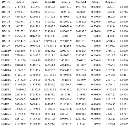
(5.1)

The raw data of 25 Indian banking

companies for the financial year 2015-16, are given in Table 1. However, the data consists of four inputs: Total operating expenses (TOE), Total demand deposits (TDD) , Total Saving deposits (TSD), Total term deposits (TTD) and three outputs: Interest income (II), Return on assets (ROA)and User fee income. From the last column of Table 1, showing overall technical efficiency scores by using Slack based measure (SBM) of efficiency given by Tone in 2001. As per the efficiency analysis DMU [1, 4, 5, 6, 7, 8, 9, 10, 12, 13, 16, 17, 18, 20, 24 and 25] are efficient DMUs. In other words, these bank branches are totally providing transaction record and have optimal value in comparison with other bank branches. While as, the remaining DMU [2, 3, 11, 14, 15, 19, 21, 22 and 23] are inefficient DMUs. This means, these bank branches are not performing well, as they have efficient score < 1 and it is equal to unity for efficient DMUs. In order to improve the efficiency score of inefficient DMUs, the reference set was determined in Table 2. The interesting fact was observe, that all efficient DMUs was not coming under the reference set, i.e., DMU [5, 6, 8, 9, 10, 12, 17, 18 and 25]. Therefore, the inefficient DMUs can benchmark these references units in order to move to words the frontier. In the second phase of this paper, we are focus on the change of efficiency score of inefficiency due changing the reference. As per the proposed NSM model for sensitivity analysis, we are excluding the reference units (efficient unit) from the reference set. Then we fund that, there is Improvement in efficiency scores to inefficient DMUs. From the table 2, ρ*

1.000(become efficient) in DMU [11 and 14] respectively by excluding DMU25 from the reference set. When DMU18 is excluding from the reference set, DMU15 improves the efficiency from 0.948 to 1.000 and become efficient. This means DMU [11, 14, and 15] are highly affected (sensitive) by excluding the DMU [25 and 18] from the reference set one by one. Same way, DMU [2 and 21] are middle sensitive

DMU. Because these DMU increases efficiency from 0.977 to 1.000 and 0.962 to 0.998 respectively, by excluding the DMU25 from the reference the set. While as, DMU [3, 19 and 23] are improving the efficiency from 0.966 to 0.987 in DMU3, 0.962 to 0.998 in DMU19 and 0.875 to 0.896 in DMU23 respectively. When DMU8, DMU25 and DMU17 are excluding from the reference set one by one.

Table 1: Input, Outputs Data, Efficiency score

DMU's Input-I Input-II Input-III Input-IV Output-I Output-II Output-III

1203

Table 2: Change of Efficiency Scores by Changing Reference DMUs

0



Reference DMUs

5 6 8 9 10 12 17 18 25

Ineffic

ient

DMUs

2 0.9766 0.9866 0.9807 0.9766 0.9766 0.9767 0.9766 0.9801 0.9766 1.0000

3 0.9657 0.9663 0.9657 0.9871 0.9657 0.9661 0.9657 0.9657 0.9657 0.9657

11 0.9433 0.9992 0.9435 0.9433 0.9551 0.9433 0.9433 0.9433 0.9433 0.9883

14 0.9595 0.9782 0.9595 0.9600 0.9595 0.9598 0.9595 0.9595 0.9595 1.0000

15 0.9481 0.9542 0.9481 0.9482 0.9549 0.9481 0.9481 0.9481 1.0000 0.9481

19 0.9924 0.9931 0.9924 0.9953 0.9924 0.9944 0.9924 0.9924 0.9924 0.9972

21 0.9621 0.9621 0.9621 0.9715 0.9625 0.9621 0.9621 0.9621 0.9621 0.9983

22 0.9882 1.0000 0.9882 0.9885 1.0000 0.9886 0.9882 0.9882 0.9882 0.9896

23 0.8747 0.8747 0.8747 0.8788 0.8843 0.8747 0.8767 0.8959 0.8747 0.8747

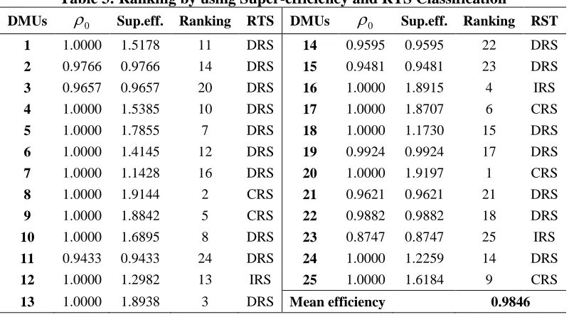
In Table 3, ρ* is overall efficiency calculated from the model (4.1) and Sup. eff. Denotes the values of Super-efficiency were the output of the model (5.1). Same time the returns to scale (RTS) classification is also mentioned in the table. This was done in the input-oriented multiplier model approach of DEA in case of VRS. The super-efficiency model is based on the input and output slacks under the assumption that all the DMUs should be perform efficiently. Finally, ranking of

DMUs was mad as per the super-efficiency score and results of Table reveals that, DMU20 is most efficient (super-efficient) from the all 25 DMUs having the super- efficiency score 1.91972. This is follow by first five positions as per ranking DMU [8, 13, 16, 9 and 17]. While as, DMU [21, 14, 15, 11 and 23] are the last five positions in the ranking. The range of the Super-efficiency is in between 0.87473 to 1.91972

and mean of the 0.9846.

Table 3: Ranking by using Super-efficiency and RTS Classification

DMUs



₀ Sup.eff. Ranking RTS DMUs



₀ Sup.eff. Ranking RST

1 1.0000 1.5178 11 DRS 14 0.9595 0.9595 22 DRS

2 0.9766 0.9766 14 DRS 15 0.9481 0.9481 23 DRS

3 0.9657 0.9657 20 DRS 16 1.0000 1.8915 4 IRS

4 1.0000 1.5385 10 DRS 17 1.0000 1.8707 6 CRS

5 1.0000 1.7855 7 DRS 18 1.0000 1.1730 15 DRS

6 1.0000 1.4145 12 DRS 19 0.9924 0.9924 17 DRS

7 1.0000 1.1428 16 DRS 20 1.0000 1.9197 1 CRS

8 1.0000 1.9144 2 CRS 21 0.9621 0.9621 21 DRS

9 1.0000 1.8842 5 CRS 22 0.9882 0.9882 18 DRS

10 1.0000 1.6895 8 DRS 23 0.8747 0.8747 25 IRS

11 0.9433 0.9433 24 DRS 24 1.0000 1.2259 14 DRS

12 1.0000 1.2982 13 IRS 25 1.0000 1.6184 9 CRS

7. Conclusions

Since DEA is linear programming based technique, sensitivity analysis is not only challenging but also very useful aspect in order to identify the sensitivity in the efficiency scores by varying the range variable. The sensitivity in DEA is not only by changing the input and output variables, but it is also due change in the reference units from the reference set. The proposed model of sensitivity analysis and super-efficiency are based on input and output slacks. As per the results of sensitivity analysis model changing the reference units DMUs from the reference set, not only the efficiencies of inefficient DMUs improves but also there is change in RTS classification. A part from this, some DMUs perform efficiently. Finally, we conclude that the reference unit of inefficient DMUs in the reference set is much more important in the aspect of sensitivity analysis to DEA. On other hand, Super-efficiency technique is only procedure for ranking of DMUs in DEA.

Acknowledgement

1205 References

[1] Agarwal, S., Yadav, S. P., and Singh, S. P. (2014). Sensitivity analysis in data envelopment analysis, International Journal of Operational Research, 19(2), 174–185.

[2] Ahn, T.S., Seiford, L.M., (1993). Sensitivity of DEA to models and variable sets in a hypothesis test setting: The efficiency operations, Quorum Books, New York, 191–208.

[3] Andersen, P., and Petersen, N.C., (1993). A procedure for ranking efficient units in data envelopment analysis, Management Science, 39, 1261–1264.

[4] Appa, G., and Williams, H. P., (2002) A formula for the solution of DEA models. Operational Research working paper, LSEOR 02.49, Department of Operational Research, London School of Economics and Political Science, London, UK.

[5] Banker, R. D., Charnes, A., and Cooper, W. W. (1984). Some models for estimating technical and scale inefficiencies in data envelopment analysis, Management Science, 30(9), 1078–1092.

[6] Charnes, A., Cooper, W. W., and Rhodes, E. (1978). Measuring the efficiency of decision making units, European Journal of Operational Research, 2(6), 429–444.

[7] Charnes, A., Cooper, W. W., Lewin, A. Y., Morey, R. C., and Rousseau, J. (1984) Sensitivity and stability analysis in DEA, Annals of Operations Research, 2(1), 139–156.

[8] Charnes, A., Neralic , L., (1989) Sensitivity analysis in data envelopment analysis 1, GlasnikMatematicki Series III, 24(44), 211–226.

[9] Charnes, A., Neralic , L., (1990). Sensitivity analysis of the additive model in data envelopment analysis, European Journal of Operational Research, 48, 332– 341.

[10] Charnes, A., Neralic, L. (1989) Sensitivity analysis in data envelopment analysis 2, Glasnik Matematicki Series III, 24(44), 449–463.

[11] Charnes, A., Neralic, L. (1992). Sensitivity analysis for the case of proportionate change of inputs (or outputs) in data envelopment analysis, Glasnik Matematicki Series III, 27(47), 191–201.

[12] Charnes, A., Neralic, L., (1992). Sensitivity analysis for the case of proportionate change of inputs (or outputs) in data envelopment analysis, Glasnik Matematicki Series III, 27(47), 393–405.

[13] Charnes, A., Zlobec, S. (1989) Stability of efficiency evaluations in data envelopment analysis, Zeitschrift fur Operations Research, 33, 167–179.

[14] Charnes, A.,Hagg, S., Jaska, P., and Semple, J. (1992). Sensitivity of efficiency classifications in the additive model of data envelopment analysis, International Journal of Systems Science, 23(5), 789–798, 1992.

[15]Dar, Q. F., Padi, T. R., and Tali, A. M. (2016). Mixed input and output orientations of data envelopment analysis with linear fractional programming and least distance measures, Statistics, Optimization and Information Computing, 4(4), 326–341.

[17] Farrell, M.J. (1957). A measurement of productive efficiency, Journal of Royal

Statistical Society Series A

(General),120(3), 253–290.

[18] Gonzalez-Lima, M.D., Tapia, R.A., and Thrall, R.M., (1996). On the construction of strong complementarity slackness solutions for DEA linear programming problems using a primal-dual interior-point method, Annals of Operations Research,66, 139–162.

[19]Jadhav, N and Ajit, D. (1996). Role of banks in the Economic Development of India, Prajnan, 25(3-4), 309–409.

[20] Jahanshahloo, G. R., Lotfi, F. H., Shoja, N., Abri, A. G., Jelodar, M. F., and Firouzabadi, K. J., (2011). Sensitivity analysis of inefficient units in data envelopment analysis, Mathematical and Computer Modelling, 53(5), 587–596.

[21] Jansen, B., De Jong, J. J., Roos, C., and Terlaky, T., (1997). Sensitivity analysis in linear programming: just be careful!, European Journal of Operational Research, 101(1), 15–28.

[22] Neralic, L., (1997). Sensitivity in data envelopment analysis for arbitrary perturbations of data, Glasnik MathematickI Series III, 32(52)315–1335.

[23] Padi, T. R., Tali, A. M., & Dar, Q. F. Multi-Period Performance Evaluation of Indian Commercial Banks Through Data Envelopment Analysis and Malmquist Productivity Index. Knowing Enough to Be Dangerous: The Dark Side of Empowering Employees with Data and Tools, 88.

[24] Seiford, L.M. and Zhu, J. (1999). Sensitivity and stability of the classification of returns to scale in data envelopment analysis, Journal of Productivity Analysis, 12(1), 55–75.

[25] Smith, P. (1997). Model

misspecification in data envelopment analysis, Annals of Operations Research,73, 233–252.

[26]Tali, A. M., Padi, T. R., and Dar, Q. F. (2017). Two-stage slack-based measure of efficiency in DEA with double frontiers, International Journal of Latest Trends in Finance and Economic Sciences, 6(3),1194–1204.

[27] Thompson, R., Dharmapala, P.S., and Thrall, R.M. (1994). Sensitivity analysis of efficiency measures with application to Kansas farming and Illinois coal mining, In: Data Envelopment Analysis: Theory, Methodology, and Applications. Springer, Dordrecht, 393–423.

[28] Thompson, R.G., Dharmapala, D.J., Gonzalez-Lima, M.D., and Thrall, R.M. (1996). DEA multiplier analytic center sensitivity with an illustrative application to independent oil companies, Annals of Operations Research, 66, 163–177.

[29]Tone, K. (2001). A slacks-based measure of efficiency in data envelopment analysis, European Journal of Operational Research, 130(3), 498–509.

[30] Wei, Q., Zhang, L.J., Zhang, X. (2000). An inverse DEA model for input/output estimate, European Journal of Operational Research, 121(1), 151–163.