Fractal Statistics and Data Roughness
1Roberto N. Padua, 2Daisy R. Palompon, 3Dexter S. Ontoy, 4Efren O. Barabat 1Consultant, Cebu Normal University
2, 3Center for Research and Development, Cebu Normal University 4University of San Jose Recoletos
Date Submitted: July 15, 2012 Originality: 83% Date Revised: March 8, 2012 Plagiarism Detection: Passed
ABSTRACT
We examine the power-law distribution with fractional exponents as a parent distribution of a random sample. The power-law distribution is shown to be similar to the Pareto distribution used in statistics for analyzing income distribution. Data roughness is described in terms of a fractal dimension (λ) which always exists even in cases where the variance (the usual measure of variability) may not exist. Estimate of data roughness for each observation xi is provided. The statistical properties of the
fractal dimension of a random variable X are explored. Visual representation of data roughness are likewise provided.
Keywords:fractals, fractal dimension, fractal integral, statistical fractals
INTRODUCTION
Fractal is a general term used to describe both the objects (geometry) and processes which exhibit self-similarity, scale invariance, fractional dimensions and heterogeneity (Mandelbrot, 1967). Its origins may be traced back quite recently to Geometry when Benoit Mandelbrot put natural roughness of objects under scrutiny: how does one describe roughness of geometric objects in nature?. The same challenge can be posed for non-geometric objects, specifically, for variables that represent certain characteristics of objects or phenomena. This area of inquiry has not been formalized and we refer to it as Fractal Statistics.
Scientific efforts to describe, explain and predict nature and natural processes are hampered by the lack of fully-developed mathematical techniques to deal with massive data irregularities and ruggedness. Mathematical statistics often assumes that the random variables of study are smooth, linearly ordered and, in most cases, regular. Nature and natural processes, on the contrary, are rugged, irregular, discontinuous and often characterized by complex, non-linear interactions (Palmer, 1992). Mandelbrot (1967) hinted on the use fractals for modeling such natural phenomena.
This paper aims to discuss foundational issues in statistical fractal analysis. Specifically, we attempt to describe “data roughness” when the conventional measure of variance cannot apply. We argue that most of the phenomena that had been modeled using the normal distribution (viz. assuming the existence of variance) can be more accurately analyzed using statistical fractals since most of them exhibit self-similar stochastic patterns. The main advantage of using statistical fractal analysis over the classical normal distribution approach is that the former respects the inherent irregularities, ruggedness and stochastic self-similarity of natural phenomena while the latter tends to smooth out the values to conform to standard methods of statistical analysis using the normal curve.
Selvam (2011) succinctly describes the shift from normal distribution approach to statistical fractals as follows: “The Gaussian probability distribution used widely for analysis and description of large data sets underestimates the probabilities of occurrence of extreme events such as stock market crashes, earthquakes, heavy rainfall, etc. The assumptions underlying the normal distribution such as fixed mean and standard deviation, independence of data, are not valid for real world fractal data sets exhibiting a scale-free power law distribution with fat tails. Fractal fluctuations therefore exhibit quantum-like chaos. The model predicted inverse power law is very close to the Gaussian distribution for small-scale fluctuations, but exhibits a fat long tail for large-scale fluctuations. Extensive data sets of Dow Jones index, Human DNA, Takifugu rubripes (Puffer fish) DNA are analysed to show that the space/time data sets are close to the model predicted power law distribution.”
Self-Similarity and Scale Invariance
Central to the study of fractals is the notion of self-similarity of an object at various scales. Horgan (1988) averred that fractals are geometric forms whose irregular details recur at different scales, that is, a fractal is a shape made of parts similar to the whole is some way (Mandelbrot, 1977). Self-similarity and scale-invariance, as described, can be translated mathematically as:
Definition1: Let 𝑓: 𝑉 → 𝑉 where V is a vector space over the field R. If: 𝑓(𝛼 𝑣) = 𝛼𝑘 𝑓(𝑣) , 𝛼, 𝑘 ∈ 𝑅+
then f is said to be scale-invariant or self-similar of order k.
In classical analysis, 𝑘 ∈ 𝑍+ is a non-negative integer and 𝑓 is called a homogeneous function of order k. However, Definition 1 allows for fractional orders. In fact, the study of fractals can be subsumed under a larger conformal symmetry analysis.
Theorem 1: If 𝑉 = 𝑅, then the only scale-invariant functions 𝑓: 𝑅 → 𝑅 are the power functions: 𝑓(𝑥) = 𝑐𝑥𝑘, 𝑐 ∈ 𝑅
where 𝑐 = 𝑓(1).
Definition 2: The fractal self-similarity dimension of an object having m copies of itself and scaled by a factor 𝑟 is:
𝜆 =log 𝑚 log 𝑟
Thus, a regular square of unit side can be reproduced 𝑚 = 4 times if we divide each side at the midpoint (𝑟 = 2). 𝐴 square will, therefore, have dimension:
𝑑 = log 4 log 2 =
2log 2
log 2 = 2 𝑎𝑠 𝑒𝑥𝑝𝑒𝑐𝑡𝑒𝑑.
The Cantor set is the traditional representation of a fractal. It is obtained by dividing the closed interval [0,1] into three and removing the middle third. The process is repeated on the two pieces [0,1
3] and [ 1
3, 1] by removing the middle third on the first piece and the middle third of the last piece and so on. The iterative process yields the set:
𝐶 = [0,1] ⋃ ⋃ (3𝑘 + 1 3𝑚 ,
3𝑘 + 1 3𝑚 ) 3𝑚−1−1
𝑘=0 ∞
𝑚=1 ⁄
which looks like “fractal dusts“. The dimension of the Cantor set is: 𝜆 =log 2
log 3= 0.63 approximately.
Nature is replete with examples of fractals. To use an example from the forest, the perimeter of a maple leaf is not smooth; it is jagged. With video imaging system, Vlcek and Cheung (1986) generated a one-pixel-thick computer image of a leaf and found the fractal dimension to be λ = 1.21 by comparing the log pixel length with the log number of lengths:
𝜆 =log 𝑁 𝜆
log 𝜆 , where 𝜆 = 𝑝𝑖𝑥𝑒𝑙 𝑙𝑒𝑛𝑔𝑡ℎ.
The usefulness of the fractal concept stems from its ability to describe apparently random structures within a precise geometry (Orbach, 1987). The study of fractals, is, therefore, inextricably linked with statistical analysis.
Fractal Statistics
The study of geometric fractals naturally leads to the study of scale-invariant probability distributions 𝑓(𝑥). In particular, we restrict our attention to a random variable X whose support is non-negative and is scale-invariant. From Theorem 1, we know that 𝑓(𝑥) has to take the form:
1…𝑓(𝑥) = 𝐴 𝑥𝜆 , 𝜃 < 𝑥 < ∞ , λ > 0
The particular power-law distribution of interest is given by: 2 …𝑓(𝑥) =𝜆−1
𝜃 ( 𝑥 𝜃)
−𝜆
after requiring that (1) be a proper density function. Equation (2) is closely related to the Pareto distribution:
3… (𝑥) = 𝜆 (𝑥 𝜃)
−𝜆 1
𝑥 , 𝜃 < 𝑥 < ∞, λ > 0. (Coelho and Mexia(2007)).
The exponent of this power distribution corresponds to the fractal dimension of X. The corresponding cumulative distribution function of X is easily shown to be:
3 …𝐹(𝑥) = 1 − (𝑥 𝜃)
1−𝜆
, 𝜃 < 𝑥 < ∞.
Power-law distributions are often used in practice when dealing with phenomena where there are more smaller values then large values of X, e.g. income distribution.
Let 𝑥1, 𝑥2, … , 𝑥𝑛 be iid 𝐹(𝑥). A maximum likelihood estimator of 𝜆 is given by: 4 …𝜆̂ = 1 + 𝑛 [∑ 𝑙𝑛 (𝑥𝑖
𝜃) 𝑛
𝑖=1 ]
−1 .
For n = 1, the maximum likelihood estimator (4) provides an “edge-roughness” indicator of the observation x:
𝜆(𝑥̂ = 1 + [𝑙𝑛 (𝑖) 𝑥𝑖 𝜃)]
−1 .
Alternatively, if we take the logarithm of both sides of Equation (2), we obtain:
5 …log 𝑓(𝑥) = 𝐶 − 𝜆 log 𝑥̇
so that a plot of 𝑙𝑜𝑔 𝑓(𝑥) versus log x yields a downward sloping line with slope 𝜆. The slope of line (5) is, therefore, an estimate of the fractal dimension of X .
Theorem 2: The only scale invariant probability distribution 𝑓(𝑥) are those for which 𝑦 = 𝑥1−𝜆 is uniformly distributed where 𝜆 is the fractal dimension of 𝑓(𝑥)
Proof: Let 𝑓(𝑥) be a scale invariant probability distribution of order 𝜆, then: 𝑓(𝛼 𝑥) = 𝛼−𝜆 𝑓(𝑥) = 1
𝛼𝜆 𝑓(𝑥). It follows that:
𝑓(𝑥 ∙ 1) = 1
𝑥𝜆 𝑓(1) or:
𝑓(𝑥) = 𝑓(1) ∙ 𝑥−𝜆 , a power – law distribution.
Let 𝑦 = 𝑥1−𝜆 so 𝑥 = 𝑦1−𝜆1 . The Jacobian of the transformation is 𝐽 = 1 1−𝜆 𝑦
𝑔(𝑦) = 𝑓 (𝑦1−𝜆 ) ∙ 1 1−𝜆 𝑦1−𝜆
= 𝑓(1) 1−𝜆∙ 𝑦
0 =𝑓(1) 1−𝜆 = 𝑘.
Since 𝑔(𝑦) is constant, it follows that y is uniformly distributed.
Moments: Mean and Variance. Classical Statistics rely heavily on the mean to characterize the general behavior of a set of data. It is a smoothing process whereby the inherent roughness of the data are removed. Its use is justified on the basis of the fact that:
6 …𝑋̅̅̅̅ → 𝜇 𝑛 𝑎𝑠 𝑛 → ∞
where 𝜇 is the population mean. However, when the observations come from a power-law distribution, then 𝑋̅̅̅̅𝑛 either continues to decrease with more observations i.e. 𝑋̅̅̅̅ → −∞ 𝑎𝑠 𝑛 →𝑛 ∞, or 𝑋̅̅̅̅𝑛 continues to increase without bound with more observations, i.e. 𝑋̅̅̅̅ → ∞ 𝑎𝑠 𝑛 → ∞.𝑛 The population mean 𝜇 does not exist when 𝜆 < 1. It will exist when 𝜆 > 1 but the variance 𝜎2 will not exist until 𝜆 reaches 2. The reliance to the Central Limit Theorem when using 𝑋̅ as an estimator of 𝜇 will have to be carefully analyzed when sampling from real data.
Since the first two (2) moments of fractal distributions may not exist, we replace them with statistical descriptive measures of roughness that always exist. To this end, define:
Definition: Let 𝛿𝜆(𝑥) = 𝑃(𝑋 ≤ 𝑥) where 𝑥 𝑑
~ 𝑓(𝑥; 𝜆), is a fractal distribution with dimension 𝜆. The 𝛼𝑡ℎ quantile of X is 𝑥
𝛼, 𝑎𝑛𝑑 𝛿𝜆(𝑥̃𝛼) = 1 − 𝛼.
The 𝛼𝑡ℎ quantile of X always exists. It is the point 𝑥̃𝛼 in the distribution such that (1 − 𝛼)𝑥 100% of the observations is below it. An explicit expression for 𝑥̃𝛼 is:
(7) 𝑥̃𝛼= 𝜃𝛼1−𝜆1 , 𝜃 < 𝑥 < ∞.
In practice, we specify 𝛼 and compute 𝑥̃𝛼. The usual choice for 𝛼 is 𝛼 =1
2 or the median, but there is no particular reason why 𝛼 should always be set equal to 1
2.
~ 1 ~ 2 1 2 the probability that an arbitrary x is less than an arbitrary y is:
(8) 𝑃(𝑥 < 𝑦) = ∫ [∫𝜃𝑦(𝜆1−1)𝜃 (𝑥 𝜃) −𝜆1 𝑑𝑥] ∞ 𝜃 [ (𝜆2−1) 𝜃 ( 𝑥 𝜃) −𝜆2 ] 𝑑𝑦
= ∫ [∫𝜃𝑦(𝜆1𝜃−1)(𝑥 𝜃) −𝜆1 𝑑𝑥] ∞ 𝜃 [ (𝜆2−1) 𝜃 ( 𝑥 𝜃) −𝜆2 ] 𝑑𝑦
= 1 + (𝜆2−1) 2−𝜆1−𝜆2 = 1 − 1−𝜆2
2−𝜆1−𝜆2
while the probability that an arbitrary x is greater than an arbitrary y is:
(9) 𝑃(𝑥 > 𝑦) = 1−𝜆2 2−𝜆1−𝜆2
Suppose that 𝜆1 = 0.2 and 𝜆2 = 0.5, then 𝑃(𝑥 < 𝑦) = 61.54% while 𝑃(𝑥 > 𝑦) = 38.46% i.e. it is more likely that an arbitrary y will be larger than an arbitrary x.
Distribution of the Sample Median. Let 𝑥1, 𝑥2, … , 𝑥𝑛 be a random sample from 𝐹(𝑋; 𝜆) and let 𝑥̃ = 𝑚𝑒𝑑𝑖𝑎𝑛 {𝑥1, 𝑥2, … , 𝑥𝑛}. Then:
(10) 𝑃(𝑋̃ ≤ 𝑥̃) = 𝑃(ℎ𝑎𝑙𝑓 𝑜𝑓 𝑡ℎ𝑒 𝑜𝑏𝑠𝑒𝑟𝑣𝑎𝑡𝑖𝑜𝑛 𝑎𝑟𝑒 𝑙𝑒𝑠𝑠 𝑡ℎ𝑎𝑛 𝑥̃)
= (𝑛𝑛 2
) 𝑃𝑛⁄2(1 − 𝑃)𝑛−𝑛 2⁄
where 𝑝 = 𝑃(𝑋 ≤ 𝑥̃) = 𝐹𝜆(𝑥̃) = 1 − ( 𝑥̃ 𝜃)
1−𝜆
and 𝑛 is even.
Hence:
(11) 𝐺(𝑥̃) = 𝑛!
(𝑛2)!(𝑛−𝑛2)![1 − ( 𝑥̃ 𝜃) 1−𝜆 ] 𝑛 2 ⁄ (𝑥̃ 𝜃)
(1−𝜆)(𝑛−𝑛 2⁄ )
We note that (11) is a Binomial distribution with parameter 𝑥̃ and n. by applying Slutsky’s Theorem, we obtain:
(12) 𝜇̃ = 𝐸(𝑥̃) and 𝑉𝑎𝑟(𝑥̃) = 1
4𝑓2(𝜇̃)where 𝜇̃ = 𝐹𝜆 −1(1
2).
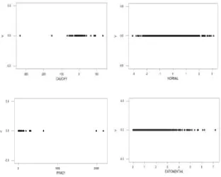
Visual Representation of Data Roughness. We generated 1000 random observations from the following distributions: N(0,1), Exponential (mean = 1), Cauchy (median = 0, s =1), and Fractal (λ = 1.63). We then plotted the observations on the x-axis to illustrate the fragmentation induced by these probability distributions:
Figure 1. Fragmentation Induced by Various Probability Distributions
The smoothest or least fragmented graph is displayed by the normal random observations where we observe a concentration of points in the middle; the most fragmented are the graphs representing the Cauchy distribution and a fractal distribution with λ = 1.63. The exponential random observations behave in a similar way as the normal observations but the concentration of points is found at the lower end of the interval. That is, the natural state of order is fractal as opposed to their normal state. In the natural state, there will be smaller variations than larger ones; more smaller values than larger values.
CONCLUSION
REFERENCES
Alhfors, C. L. (1990) Functions of Complex Variables. (Wiley Series: New York)
Barnsley, Michael F.; and Rising, Hawley; Fractals Everywhere. Boston: Academic Press Professional, 1993.
Ben-Avraham, Daniel; Havlin, Shlomo (2000). Diffusion and Reactions in Fractals and Disordered Systems. Cambridge University
Bunge, Mario. 1968. The Maturation of Science. In: Lakatos, I.; Musgrove, A., eds. Problems in the philosophy of science. Amsterdam: North – Holand: 120 – 147.
Burrough, P.A. 1981. Fractal dimensions landscape and other environment data. Nature. 294: 240 – 242.
Burrough, P.A. 1983a. Multiscale sources of spatial variation in soil. I. The application of fractal concepts to nested levels of soil variation. Journal of Soil Science. 34: 571 – 597.
Burrough, P.A. 1983b. Multiscale sources of spatial variation in soil. II. A non – Brownian fractal model and its application in soil survey. Journal of Soil Science. 34: 599 – 620.
Burrough, P.A. 1985. Flakes, Facsimiles and facts: fratal models of geophysical phenomena. In: Nash, S., ed. Science and uncertainty. Middlesex England: Science Reviews: 150-169.
Campbell, David.1989. An introduction to non-linear dynamics. In: Stein, D.L.,eds. Lectures in sciences of complexity. Menlo Park. CA: Addison – Wesley: 3-106.
Coelho, C. and Mexia, J. (2007) On the distribution of the Product and Ratio of Independent Generalized Gamma-Ratio Random Variables. (Sankhya: The Indian Journal of Statistics, Vol. 69, pp. 221-255).
Crow, T.R. 1990. Old growth and biological diversity: a basis for sustainable forestry. In: Old growth forests: what are they? How do they works? Toronto, Canada: Canadian Scholars’ Press. 197 p.
Devancy, Robert L. 1990. Chaos, fractals and dynamics: computer experiments in mathematics. Menlo Park, CA: Adison –Wesley. 178 p.
Devaney, Robert L. 1988. Fractal patterns arising in chaotic dynamical systems. In: Peitgen, H.O.; Saupe, D., eds. The science of fractal images. New York, NY: Springer – Verlag: 137 – 168.
Gouyet, Jean-François; Physics and Fractal Structures (Foreword by B. Mandelbrot); Masson, 1996. ISBN 2-225-85130-1, and New York: Springer-Verlag, 1996.
Hardwick, Richard C. 1990. Ecological power laws. Nature. 343 – 420.
Hausdorff, F. 1919. Dimension und ausseres Mass. Mathematische Annalen. 79: 157 – 179.
Ito, K., ed. 1987. Encyclopedic dictionary of mathematics. 4 vol. 2nd ed. Cambridge, MA: Mathematical Society of Japan. MIT Press. 2,148 p.
Jones, Jesse; Fractals for the Macintosh, Waite Group Press, Corte Madera, CA, 1993.
Jonot, P.G.: McNaughton, K.G. 1986. Some remarks on the Hausdorff dimension. In: Cherbit, G., ed. Fractals: non-integral dimensions and applications. New York, NY:John Wiley and Sons: 103 – 119.
Jürgens, Hartmut; Peitgen, Heins-Otto; and Saupe, Dietmar; Chaos and Fractals: New Frontiers of Science. New York: Springer-Verlag, 1992.
Khilmi, G.F. 1962. Theoretical forest biogeophysics. Jerusalem, Israel: Israel Program for Scientific Translations. 155 p.
Kramer, E.E. 1970. The nature and growth of modern mathematics. New York, NY: Hawthorn. 758 p.
Krummel, J.R. 1986. Landscape ecology: spatial data and analytical approaches. In: Dyer, M.I.; Crossley, D.A., eds. coupling of ecological studies with remote sensing: potentials at four biosphere reserves in the United State. U.S. Man and the Biosphere Prog. Publ. 9504. Wshington, DC: Department of State.
Krummel,J.R.; Gardner, R.H.; Sugihara, G.; O’Neill,R.V.; Coleman, P.R. 1987. Landscape patterns in a disturbed environment. Oikos. 48: 321 – 324.
Lauwerier, Hans; Fractals: Endlessly Repeated Geometrical Figures, Translated by Sophia Gill-Hoffstadt, Princeton University Press, Princeton NJ, 1991.
Lesmoir-Gordon, Nigel; "The Colours of Infinity: The Beauty, The Power and the Sense of Fractals."
Liu, Huajie; Fractal Art, Changsha: Hunan Science and Technology Press, 1997,
Peitgen, Heinz-Otto; and Saupe, Dietmar; eds.; The Science of Fractal Images. New York: Springer-Verlag, 1988.
Pickover, Clifford A.; ed.; Chaos and Fractals: A Computer Graphical Journey - A 10 Year Compilation of Advanced Research. Elsevier, 1998.
Selvam, A.M. (2008) “Fractal Fluctuations and Statistical Normal Distribution” (Retrieved March 16, 2013 in arxiv.org/pdf/0805.3426)
Sprott, Julien Clinton (2003). Chaos and Time-Series Analysis. Oxford University Press.