Choosing Multiple Parameters for Support
Vector Machines
OLIVIER CHAPELLE [email protected]
LIP6, Paris, France
VLADIMIR VAPNIK [email protected]
AT&T Research Labs, 200 Laurel Ave, Middletown, NJ 07748, USA
OLIVIER BOUSQUET [email protected]
´
Ecole Polytechnique, France
SAYAN MUKHERJEE [email protected]
MIT, Cambridge, MA 02139, USA Editor: Nello Cristianini
Abstract. The problem of automatically tuning multiple parameters for pattern recognition Support Vector Machines (SVMs) is considered. This is done by minimizing some estimates of the generalization error of SVMs using a gradient descent algorithm over the set of parameters. Usual methods for choosing parameters, based on exhaustive search become intractable as soon as the number of parameters exceeds two. Some experimental results assess the feasibility of our approach for a large number of parameters (more than 100) and demonstrate an improvement of generalization performance.
Keywords: support vector machines, kernel selection, leave-one-out procedure, gradient descent, feature selection
1. Introduction
In the problem of supervised learning, one takes a set of input-output pairsZ = {(x1,y1),
. . . , (x,y)}and attempts to construct a classifier function f that maps input vectorsx∈X
onto labelsy∈Y. We are interested here in pattern recognition or classification, that is the case where the set of labels is simplyY = {−1,1}. The goal is to find a f∈F which minimizes the error (f(x)= y) on future examples. Learning algorithms usually depend on parameters which control the size of the classFor the way the search is conducted inF. Several techniques exist for performing the selection of these parameters. The idea is to find the parameters that minimize the generalization error of the algorithm at hand. This error can be estimated either via testing on some data which has not been used for learning (hold-out testing or cross-validation techniques) or via a bound given by theoretical analysis. Tuning multiple parameters. Usually there are multiple parameters to tune at the same time and moreover, the estimates of the error are not explicit functions of these parameters, so
that the naive strategy which is exhaustive search in the parameter space becomes intractable since it would correspond to running the algorithm on every possible value of the parameter vector (up to some discretization). We propose here a methodology for automatically tuning multiple parameters for the Support Vector Machines (SVMs) which takes advantage of the specific properties of this algorithm.
The SVM algorithm. Support vector machines (SVMs) realize the following idea: map a n-dimensional input vectorx∈Rn1into a high dimensional (possibly infinite dimensional)
feature spaceHbyand construct an optimal separating hyperplane in this space. Different mappings construct different SVMs.
When the training data is separable, the optimal hyperplane is the one with the maximal distance (inHspace) between the hyperplane and the closest image(xi)of the vectorxi
from the training data. For non-separable training data a generalization of this concept is used.
Suppose that the maximal distance is equal toγand that the images(x1), . . . , (x)of the training vectorsx1, . . . ,xare within a sphere of radiusR. Then the following theorem holds true (Vapnik & Chapelle, 2000).
Theorem 1. Given a training set Z = {(x1,y1), . . . , (x,y)}of size,a feature space Hand a hyperplane(w,b),the marginγ (w,b,Z)and the radius R(Z)are defined by
γ (w,b,Z)= min
(xi,yi)∈Z
yi(w·(xi)+b)
w
R(Z)=min
a,xi
(xi)+a
The maximum margin algorithm L:(X×Y)→H×Rtakes as input a training set of size
and returns a hyperplane in feature space such that the marginγ (w,b,Z)is maximized. Note that assuming the training set separable means thatγ >0. Under this assumption,for all probability measures P underlying the data Z,the expectation of the misclassification probability
perr(w,b)=P(sign(w·(X)+b)=Y)
has the bound
E{perr(L−1(Z))} ≤
1
E
R2(Z)
γ2(L(Z),Z)
.
The expectation is taken over the random draw of a training set Z of size−1for the left hand side and sizefor the right hand side.
This theorem justifies the idea of constructing a hyperplane that separates the data with a large margin: the larger the margin the better the performance of the constructed hyperplane.
Note however that according to the theorem the average performance depends on the ratio E{R2/γ2}and not simply on the large marginγ.
Why multiple parameters? The SVM algorithm usually depends on several parameters. One of them, denoted C, controls the tradeoff between margin maximization and error minimization. Other parameters appear in the non-linear mapping into feature space. They are called kernel parameters. For simplicity, we will use a classical trick that allows us to consider C as a kernel parameter, so that all parameters can be treated in a unified framework.
It is widely acknowledged that a key factor in an SVM’s performance is the choice of the kernel. However, in practice, very few different types of kernels have been used due to the difficulty of appropriately tuning the parameters. We present here a technique that allows to deal with a large number of parameters and thus allows to use more complex kernels.
Another potential advantage of being able to tune a large number of parameters is the possibility of rescaling the attributes. Indeed, when no a priori knowledge is available about the meaning of each of the attributes, the only choice is to use spherical kernels (i.e. give the same weight to each attribute). But one may expect that there is a better choice for the shape of the kernel since many real-world database contain attributes of very different natures. There may thus exist more appropriatescaling factorsthat give the right weight to the right feature. For example, we will see how to use radial basis function kernels (RBF) with as many different scaling factors as input dimensions:
K(x,z)=exp
−
i
(xi−zi)2
2σi2
.
The usual approach is to considerσ =σ1 = · · · =σn and to try to pick the best value for
σ. However, using the proposed method, we can choose automatically good values for the scaling factorsσi. Indeed, these factors are precisely parameters of the kernel.
Moreover, we will demonstrate that the problem offeature selectioncan be addressed with the same framework since it corresponds to finding those attributes which can be rescaled with a zero factor without harming the generalization.
We thus see that tuning kernel parameters is something extremely useful and a procedure that allows to do this would be a versatile tool for various tasks such as finding the right shape of the kernel, feature selection, finding the right tradeoff between error and margin, etc. All this gives a rationale for developing such techniques.
Our approach. In summary, our goal is not only to find the hyperplane which maximizes the margin but also the values of the mapping parameters that yield best generalization error. To do so, we propose a minimax approach: maximize the margin over the hyperplane coefficients and minimize an estimate of the generalization error over the set of kernel parameters. This last step is performed using a standard gradient descent approach. What kind of error estimates. We will consider several ways of assessing the generalization error.
• Validation error: this procedure requires a reduction of the amount of data used for learning in order to save some of it for validation. Moreover, the estimates have to be smoothed for proper gradient descent.
• Leave-one-out error estimates: this procedure gives an estimate of the expected general-ization as an analytic function of the parameters.
We will examine how the accuracy of the estimates influences the whole procedure of finding optimal parameters. In particular we will show that what really matters is how variations of the estimates relate to variations of the test error rather than how their values are related. Outline. The paper is organized as follows. The next section introduces the basics of SVMs. The different possible estimates of their generalization error are described in Sections 3 and 4 explains how to smooth theses estimates. Then we introduce in Section 5 a framework for minimizing those estimates by gradient descent. Section 6 deals with the computation of gradients of error estimates with respect to kernel parameters. Fi-nally, in Sections 7 and 8, we present experimental results of the method applied to a variety of databases in different contexts. Section 7 deals with finding the right penalization along with the right radius for a kernel and with finding the right shape of a kernel. In Section 8 we present results of applying our method to feature selection.
2. Support vector learning
We introduce some standard notations for SVMs; for a complete description, see (Vapnik, 1998). Let{(xi,yi)}1≤i≤be a set of training examples,xi ∈ Rn which belong to a class
labeled by yi ∈ {−1,1}. In the SVM methodology, we map these vectors into a feature
space using a kernel functionK(xi,xj)that defines an inner product in this feature space.
Here, we consider a kernel Kθθθdepending on a set of parametersθ. The decision function given by an SVM is:
f(x)=sign
i=1 α0
iyiKθθθ(xi,x)+b
, (1)
where the coefficientsαi0are obtained by maximizing the following functional:
W(α)=
i=1 αi−
1 2
i,j=1
αiαjyiyjKθθθ(xi,xj) (2)
under the constraints
i=1
αiyi =0 and αi≥0, i =1, . . . , .
The coefficients α0
i define a maximal margin hyperplane in a high-dimensional feature
space where the data are mapped through a non-linear functionsuch that(xi)·(xj)=
This formulation of the SVM optimization problem is called thehard marginformulation since no training errors are allowed. Every training point satisfies the inequalityyif(xi)≥1
and for pointsxiwith correspondingαi >0 an equality is satisfied. These points are called
support vectors.
Notice that one may require the separating hyperplane to pass through the origin by choosing a fixedb =0. This variant is called the hard margin SVMwithout threshold. In that case, the optimization problem remains the same as above except that the constraint
αiyi =0 disappears.
Dealing with non-separability. For the non-separable case, one needs to allow training errors which results in the so calledsoft marginSVM algorithm (Cortes & Vapnik, 1995). It can be shown that soft margin SVMs with quadratic penalization of errors can be considered as a special case of the hard margin version with the modified kernel (Cortes & Vapnik, 1995; Cristianini & Shawe-Taylor, 2000).
K←K+ 1
CI, (3)
whereIis the identity matrix andCa constant penalizing the training errors. In the rest of the paper, we will focus on the hard margin SVM and use (3) whenever we have to deal with non-separable data. ThusCwill be considered just as another parameter of the kernel function.
3. Estimating the performance of an SVM
Ideally we would like to choose the value of the kernel parameters that minimize the true risk of the SVM classifier. Unfortunately, since this quantity is not accessible, one has to build estimates or bounds for it. In this section, we present several measures of the expected error rate of an SVM.
3.1. Single validation estimate
If one has enough data available, it is possible to estimate the true error on a validation set. This estimate is unbiased and its variance gets smaller as the size of the validation set increases. If the validation set is{(xi,yi)}1≤i≤p, the estimate is
T = 1 p
p
i=1
(−y
if(xi)), (4)
3.2. Leave-one-out bounds
The leave-one-out procedure consists of removing from the training data one element, constructing the decision rule on the basis of the remaining training data and then testing on the removed element. In this fashion one tests allelements of the training data (using different decision rules). Let us denote the number of errors in the leave-one-out procedure byL(x1,y1, . . . ,x,y). It is known (Luntz & Brailovsky, 1969) that the the leave-one-out procedure gives an almost unbiased estimate of the expected generalization error:
Lemma 1.
E perr−1=
1
E(L(x1,y1, . . . ,x,y)),
where p−1
err is the probability of test error for the machine trained on a sample of size−1
and the expectations are taken over the random choice of the sample.
Although this lemma makes the leave-one-out estimator a good choice when estimating the generalization error, it is nevertheless very costly to actually compute since it requires running the training algorithmtimes. The strategy is thus to upper bound or approximate this estimator by an easy to compute quantityT having, if possible, an analytical expression. If we denote by f0the classifier obtained when all training examples are present and fi the one obtained when exampleihas been removed, we can write:
L(x1,y1, . . . ,x,y)=
p=1
(−ypfp(xp)), (5)
which can also be written as L(x1,y1, . . . ,x,y)=
p=1
(−ypf0(xp)+yp(f0(xp)− fp(xp))).
Thus, ifUp is an upper bound foryp(f0(xp)− fp(xp)), we will get the following upper
bound on the leave-one-out error: L(x1,y1, . . . ,x,y)≤
p=1
(Up−1),
since for hard margin SVMs,ypf0(xp)≥1 and is monotonically increasing.
3.2.1. Support vector count. Since removing a non-support vector from the training set
does not change the solution computed by the machine (i.e.Up = f0(xp)− fp(xp)=0
bound each term in the sum by 1 which gives the following bound on the number of errors made by the leave-one-out procedure (Vapnik, 1995):
T = NSV
,
whereNSV denotes the number of support vectors.
3.2.2. Jaakkola-Haussler bound. For SVMs without threshold, analyzing the
optimiza-tion performed by the SVM algorithm when computing the leave-one-out error, Jaakkola and Haussler (1999) proved the inequality:
yp(f0(xp)− fp(xp))≤α0pK(xp,xp)=Up
which leads to the following upper bound:
T = 1
p=1 α0
pK(xp,xp)−1 .
Note that Wahba, Lin, and Zhang (2000) proposed an estimate of the number of errors made by the leave-one-out procedure, which in the hard margin SVM case turns out to be
T =α0pK(xp,xp),
which can be seen as an upper bound of the Jaakkola-Haussler one since(x−1)≤xfor x≥0.
3.2.3. Opper-Winther bound. For hard margin SVMs without threshold, Opper and
Winther (2000) used a method inspired from linear response theory to prove the following: under the assumption that the set of support vectors does not change when removing the example p, we have
yp(f0(xp)− fp(xp))=
α0
p
K−SV1 pp
,
whereKSV is the matrix of dot products between support vectors; leading to the following
estimate:
T = 1
p=1
α0
p
K−SV1 pp
−1
.
3.2.4. Radius-margin bound. For SVMs without threshold and with no training errors, Vapnik (1998) proposed the following upper bound on the number of errors of the leave-one-out procedure:
T = 1
R2 γ2.
whereRandγare the radius and the margin as defined in Theorem 1.
3.2.5. Span bound. Vapnik and Chapelle (2000) and Chapelle and Vapnik (1999) derived
an estimate using the concept ofspanof support vectors.
Under the assumption that the set of support vectors remains the same during the leave-one-out procedure, the following equality is true:
yp(f0(xp)− fp(xp))=α0pS2p,
whereSpis the distance between the point(xp)and the setpwhere
p =
i=p, α0
i>0
λi(xi),
i=p
λi =1
. (6)
This gives the exact number of errors made by the leave-one-out procedure under the previous assumption:
T = 1
p=1 α0
pS2p−1 . (7)
The span estimate can be related to other approximations:
Link with Jaakkola-Haussler bound. If we consider SVMs without threshold, the con-straintλi=1 can be removed in the definition of the span. Then we can easily upper
bound the value of the span:S2p≤K(xp,xp), and thus recover the Jaakkola-Haussler bound.
Link with R2/γ2. For each support vector, we have y
pf0(xp)=1. Since for x≥0,
(x−1)≤x, the number of errors made by the leave-one-out procedure is bounded by:
p
α0
pS2p.
It has been shown (Vapnik & Chapelle, 2000) that the spanSpis bounded by the diameter
of the smallest sphere enclosing the training points and sinceα0p =1/γ2, we finally get
T ≤4R
2 γ2.
A similar derivation as the one used in thespan boundhas been proposed in Joachims (2000), where the leave-one-out error is bounded by|{p,2α0
pR2>ypf0(xp)}|, with 0≤K(xi,xi)≤
R2,∀i.
Link with Opper-Winther. When the support vectors do not change, the hard margin case without threshold gives the same value as the Opper-Winther bound, namely:
S2p =
1
K−SV1 pp
.
4. Smoothing the test error estimates
The estimate of the performance of an SVM through a validation error (4) or the leave-one-out error (5) requires the use of the step function. However, we would like to use a gradient descent approach to minimize those estimates of the test error. Unfortunately the step function is not differentiable. As already mentioned in Section 3.2.5, it is possible to bound(x−1)byxforx≥0. This is how the boundR2/γ2is derived from the
leave-one-out error. Nevertheless by doing so, large errors count more than one, therefore it might be advantageous instead to use a contracting function of the form(x)=(1+exp(−Ax + B))−1(see figure 1).
However, the choice of the constants AandBis difficult. If Ais too small, the estimate is not accurate andAis too large, the resulting estimate is not smooth.
Instead of trying to pick good constants AandB, one can try to get directly a smooth approximation of the test error by estimating posterior probabilities. Recently, Platt proposed the following estimate of the posterior distributionP(Y=1|X=x)of an SVM outputf(x)
(Platt, 2000): ˜
PA,B(x)= ˜P(Y=1|X=x)=
1
1+exp(A f(x)+B),
where f(x)is the output of the SVM. The constants AandBare found by minimizing the Kullback-Leibler divergence between P˜and an empirical approximation ofPbuilt from a validation set(xi,yi)1≤i≤nv:
(A∗,B∗)=arg max
A,B nv
i=1
1+yi
2 log(P˜A,B(x
i))+
1−yi
2 log(1− ˜PA,B(x
i))
.
This optimization is carried out using a second order gradient descent algorithm (Platt, 2000). According to this estimate the best threshold for our SVM classifier f is such that f(x)=sign(P˜A∗,B∗(x)−0.5). Note that ifB∗=0, we obtained a correction compared to
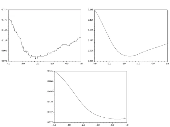
Figure 1. Validation error for different values of the width (in log scale) of an RBF kernel. Top left: with a step function,(x)=1x>0. Top right: sigmoid function,(x)=(1+exp(−5x))−1. Bottom: linear function, (x)=1+xforx>−1, 0 otherwise. Note that on the bottom picture, the minimum is not at the right place.
By definition the generalization error of our classifier is P(Y = f(X))=
x,f(x)=−1
P(Y =1|x)dµ(x)+
x,f(x)=1
(Y = −1|x)dµ(x).
This error can be empirically estimated as2:
P(Y = f(X))≈
i,P˜(xi)<0.5
˜ P(xi)+
i,P˜(xi)>0.5
1− ˜P(xi) (8)
=
nv
i=1
min(P˜(xi),1− ˜P(xi)). (9)
Note that the labels of the validation set are not used directly in this last step but indirectly through the estimation of the constantsAandBappearing in the parametric form ofP˜A∗,B∗.
To have a better understanding of this estimate, let us consider the extreme case where there is no error on the validation set. Then the maximum likelihood algorithm is going to yield A= −∞andP˜A∗,B∗(x)will only take binary values. As a consequence, the estimate of the
5. Optimizing the kernel parameters
Let’s go back to the SVM algorithm. We assume that the kernelkdepends on one or several parameters, encoded into a vectorθ =(θ1, . . . , θn). We thus consider a class of decision
functions parametrized byα,bandθ: fαα,b,θθθ(x)=sign
i=1
αiyiKθθθ(x,xi)+b
.
We want to choose the values of the parametersαandθsuch thatW (see Eq. (2)) is maximized (maximum margin algorithm) andT, the model selection criterion, is minimized (best kernel parameters). More precisely, forθfixed, we want to haveα0=arg maxW(α)
and chooseθ0such that
θ0=arg min
θθθ T(α 0,θ).
Whenθis a one dimensional parameter, one typically tries a finite number of values and picks the one which gives the lowest value of the criterionT. When bothT and the SVM solution are continuous with respect toθ, a better approach has been proposed by Cristianini, Campbell, and Shawe-Taylor (1999): using an incremental optimization algorithm, one can train an SVM with little effort whenθis changed by a small amount. However, as soon as θhas more than one component computingT(α,θ)for every possible value ofθbecomes intractable, and one rather looks for a way to optimizeT along a trajectory in the kernel parameter space.
Using the gradient of a model selection criterion to optimize the model parameters has been proposed in Bengio (2000) and demonstrated in the case of linear regression and time-series prediction. It has also been proposed by Larsen et al. (1998) to optimize the regularization parameters of a neural network.
Here we propose an algorithm that alternates the SVM optimization with a gradient step is the direction of the gradient ofT in the parameter space. This can be achieved by the following iterative procedure:
1. Initialize θ to some value.
2. Using a standard SVM algorithm, find the maximum of the
quadratic form W:
α0(θ)=arg max
ααα W(α,θ).
3. Update the parameters θ such that T is minimized.
This is typically achieved by a gradient step (see below).
4. Go to step 2 or stop when the minimum of T is reached.
Solving step 3 requires estimating howT varies withθ. We will thus restrict ourselves to the case whereKθθθcan be differentiated with respect toθ. Moreover, we will only consider cases where the gradient ofT with respect toθcan be computed (or approximated).
Note thatα0depends implicitly onθsinceα0is defined as the maximum ofW. Then, if
we havenkernel parameters(θ1, . . . , θn), the total derivative ofT0(·)≡T(α0(·),·)with
respect toθp is:
∂T0
∂θp
= ∂T0
∂θp
ααα0fixed
+∂T0
∂α0 ∂α0
∂θp
.
Having computed the gradient∇θθθT(α0,θ), a way of performing step 3 is to make a
gradient step:
δθk= −ε∂
T(α0,θ) ∂θk
,
for some small and eventually decreasingε. The convergence can be improved with the use of second order derivatives (Newton’s method):
δθk= −(θθθT)−1∂
T(α0,θ) ∂θk
where the Laplacian operatoris defined by
(θθθT)i,j= ∂
2T(α0,θ) ∂θi∂θj
.
In this formulation, additional constraints can be imposed through projection of the gradient.
6. Computing the gradient
In this section, we describe the computation of the gradient (with respect to the kernel parameters) of the different estimates of the generalization error. First, for the boundR2/γ2
(see Theorem 1), we obtain a formulation of the derivative of the margin (Section 6.1) and of the radius (Section 6.2). For the validation error (see Eq. (4)), we show how to calculate the derivative of the hyperplane parametersα0andb(see Section 6.3). Finally, the computation
of the derivative of the span bound (7) is presented in Section 6.4. We first begin with a useful lemma.
Lemma 2. Suppose we are given a(n×1)vectorvθ and an(n×n)matrixPθsmoothly depending on a parameterθ. Consider the function:
L(θ)=max
x∈F x T
vθ−1
2x
T
Pθx
where
Letx¯be the the vectorxwhere the maximum in L(θ)is attained. If this minimum is unique then
∂L(θ)
∂θ = ¯x
T∂vθ
∂θ −
1 2x¯
T∂Pθ
∂θ x¯.
In other words,it is possible to differentiate L with respect toθas ifx¯did not depend on
θ. Note that this is also true if one(or both)of the constraints in the definition of F are removed.
Proof: We first need to express the equality constraint with a Lagrange multiplierλand the inequality constraints with Lagrange multipliersγi:
L(θ)=max
x,λ,γ x
T
vθ−1
2x
T
Pθx−λ(bTx−c)+γTx. (10)
At the maximum, the following conditions are verified:
vθ−Pθx¯ = ¯λb− ¯γ , bTx¯ =c,
¯
γix¯i =0, ∀i.
We will not consider here differentiability problems. The interested reader can find de-tails in Bonnans and Shapiro (2000). The main result is that wheneverx¯ is unique, L is differentiable.
We have
∂L(θ)
∂θ = ¯x
T∂vθ
∂θ −
1 2x¯
T∂Pθ
∂θ x¯+ ∂x¯T
∂θ (vθ−Pθx¯),
where the last term can be written as follows,
∂x¯T
∂θ (vθ−Pθx¯)= ¯λ ∂x¯T
∂θ b−
∂x¯T
∂θ γ .¯
Using the derivatives of the optimality conditions, namely
∂x¯T
∂θ b=0, ∂γ¯i
∂θ x¯i+ ¯γi
∂x¯i
∂θ =0,
and the fact that eitherγ¯i =0 orx¯i =0 we get:
∂γ¯i
∂θ x¯i = ¯γi
∂x¯i
hence
∂x¯T
∂θ (vθ−Pθx¯)=0
and the result follows. ✷
6.1. Computing the derivative of the margin
Note that in feature space, the separating hyperplane{x:w·(x)+b=0}has the following expansion
w=
i=1 α0
iyi(xi)
and is normalized such that min
1≤i≤yi(w·(xi)+b)=1.
It follows from the definition of the margin in Theorem 1 that this latter isγ=1/w. Thus
we write the boundR2/γ2asR2w2.
The previous lemma enables us to compute the derivative of w2. Indeed, it can be shown (Vapnik, 1998) that
1 2w
2=W(α0),
and the lemma can be applied to the standard SVM optimization problem (2), giving
∂w2 θp
= −
i,j=1 α0
iα0jyiyj∂
K(xi,xj)
∂θp
6.2. Computing the derivative of the radius
Computing the radius of the smallest sphere enclosing the training points can be achieved by solving the following quadratic problem (Vapnik, 1998):
R2=max
βββ
i=1
βiK(xi,xi)−
i,j=1
βiβjK(xi,xj)
under constraints
i=1 βi =1
We can again use the previous lemma to compute the derivative of the radius:
∂R2 ∂θp =
i=1 β0
i
∂K(xi,xi)
∂θp −
i,j=1 βiβj
∂K(xi,xj)
∂θp ,
whereβ0maximizes the previous quadratic form.
6.3. Computing the derivative of the hyperplane parameters
Let us first compute the derivative ofα0with respect to a parameterθ of the kernel. For
this purpose, we need an analytical formulation forα0. First, we suppose that the points
which are not support vectors are removed from the training set. This assumption can be done without any loss of generality since removing a point which is not support vector does not affect the solution. Then, the fact that all the points lie on the margin can be written
KY Y
YT 0
H
α0
b
=
1
0
,
whereKYij =yiyjK(xi,xj). If there arensupport vectors,His a(n+1)×(n+1)matrix.
The parameters of the SVMs can be written as:
(α0,b)T =
H−1(1· · ·1 0)T.
We are now able to compute the derivatives of those parameters with respect to a kernel parameterθp. Indeed, since the derivative of the inverse of a matrix M depending on a
parameterθpcan be written3
∂M−1 ∂θp
= −M−1∂M ∂θp
M−1, (11)
it follows that
∂(α0,b) ∂θp
= −H−1∂H ∂θp
H−1(1· · ·1 0)T, and finally
∂(α0,b) ∂θp
= −H−1∂H ∂θp
We can easily use the result of this calculation to recover the computation ∂∂θw2
p . Indeed, if
we denoteα˜ =(α0,b), we havew2=(α0)TKYα0= ˜αT
Hα˜ and it turns out that:
∂w2 ∂θp
= ˜αT∂H
∂θp
˜
α+2α˜H∂α˜ ∂θp
= ˜αT∂H
∂θp
˜
α−2α˜HH−1∂H ∂θp
˜ α = − ˜αT∂H
∂θp ˜
α = −(α0)T∂K
Y
∂θp
α0.
6.4. Computing the derivative of the span-rule
Now, let us consider the span value. Recall that the span of the support vectorxpis defined
as the the distance between the point(xp)and the setpdefined by (6). Then the value
of the span can be written as:
S2p =min
λλλ maxµ
(xp)−
i=p
λi(xi)
2
+2µ
i=p
λi−1
.
Note that we introduced a Lagrange multiplierµto enforce the constraintλi =1.
Introducing the extended vectorλ˜ =(λTµ)Tand the extended matrix of the dot products
between support vectors ˜
KSV =
K 1
1T 0
,
the value of the span can be written as: S2p =min
λλλ maxµ (K(xp,xp)−2v
Tλ˜ + ˜λT
Hλ˜),
whereHis the submatrix ofK˜SVwith row and columnpremoved, andvis thep-th column
ofK˜SV.
From the fact that the optimal value ofλ˜ isH−1v, it follows: S2p =K(xp,xp)−vTH−1v
The last equality comes from the following block matrix identity, known as the “Woodbury” formula (L¨utkepohl, 1996)
A1 AT
A A2
−1
=
B1 BT
B B2
,
whereB1=(A1−AA−21A
T)−1.
The closed form we obtain is particularly attractive since we can compute the value of the span for each support vector just by inverting the matrixKSV.
Combining Eqs. (12) and (11), we get the derivative of the span
∂S2
p
∂θp
=S4p
˜
K−SV1∂K˜SV θp
˜
K−SV1
pp
Thus, the complexity of computing the derivative of the span-rule with respect to a parameterθp of the kernel requires only the computation of ∂
K(xi,xj)
∂θp and the inversion of
the matrixK˜SV. The complexity of these operations is not larger than that of the quadratic
optimization problem itself.
There is however a problem in this approach: the value given by the span-rule is not continuous. By changing smoothly the value of the parametersθ, the coefficientsαpchange
continuously, but the span S2
p does not. There is actually a discontinuity for most support
vectors when the set of support vectors changes. This can be easily understood from Eq. (6): suppose that upon changing the value of the parameter fromθtoθ+ε, a pointxmis not a
support vector anymore, then for all other support vectors(xp)p=m, the setp is going to
be smaller and a discontinuity is likely to appear for the value ofSp=d((xp), p).
The situation is explained in figure 2: we plotted the value of the span of a support vector
xpversus the width of an RBF kernelσ. Almost everywhere the span is decreasing, hence a
negative derivative, but some jumps appear, corresponding to a change in the set of support vectors. Moreover the span is globally increasing: the value of the derivate does not give us a good indication of the global evolution of the span.
One way to solve is this problem is to try to smooth the behavior of the span. This can be done by imposing the following additional constraint in the definition ofpin Eq. (6):
|λi| ≤ cαi0, wherecis a constant. Given this constraint, if a pointxmis about to leave or
has just entered the set of support vectors, it will not have a large influence on the span of the other support vectors, sinceα0
mwill be small. The effect of this constraint is to make
the setpbecome “continuous” when the set of support vectors changes.
However this new constraint prevents us from computing the span as efficiently as in Eq. (12). A possible solution is to replace the constraint by a regularization term in the computation of the span:
S2p = min
λλλ,λi=1
(xp)− n
i=p
λi(xi)
2 +η n
i=p
1
α0
i
λ2
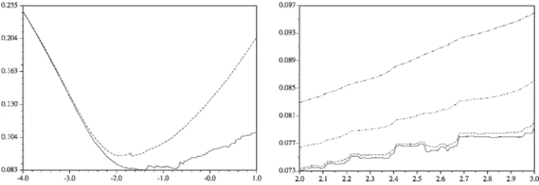
Figure 2. Value ofS2
p, the sum of the span of the training points for different values of the width of an RBF
kernel varying in the small vicinity.
With this new definition of the span, Eq. (12) becomes: S2p =1/(K˜SV +D)−pp1−Dpp,
whereDis a diagonal matrix with elementsDii =η/αi0andDn+1,n+1 =0. As shown on
figure 3, the span is now much smoother and its minimum is still at the right place. In our experiments, we tookη=0.1.
Note that computing the derivative of this new expression is no more difficult than the previous span expression.
Figure 3. Left: the minima of the span prediction with regularization (dashed line) and without regular-ization (solid line) are close. Right: detailed behavior of the span for different values of the regularizer,
It is interesting to look at the leave-one-out error for SVMs without threshold. In this case, the value of the span with regularization writes:
S2p =min
λλλ
(xp)−
i=p
λi(xi)
2
+η
n
i=p
1
α0
i
λ2
i
As already pointed out in Section 3.2.5, ifη=0, the value of span is: S2p =
1
K−SV1 pp.
and we recover the Opper-Winther bound.
On the other hand, ifη= +∞, thenλ=0 andS2
p =K(xp,xp). In this case, the span
bound is identical to the Jaakkola-Haussler one.
In a way, the span bound with regularization is in between the bounds of Opper-Winther and Jaakkola-Haussler.
7. Experiments
Experiments have been carried out to assess the performance and feasibility of our method. The first set of experiments consists in finding automatically the optimal value of two parameters: the width of an RBF kernel and the constantCin Eq. (3). The second set of experiments corresponds to the optimization of a large number of scaling factors in the case of handwritten digit recognition. We then show that optimizing scaling factors leads naturally to feature selection and demonstrate the application of the method to the selection of relevant features in several databases.
7.1. Optimization details
The core of the technique we present here is a gradient descent algorithm. We used the optimization toolbox of Matlab to perform it. It includes second order updates to improve the convergence speed. Since we are not interested in the exact value of the parameters minimizing the functional, we used a loose stopping criterion.
7.2. Benchmark databases
In a first set of experiments, we tried to select automatically the widthσ of a RBF kernel,
K(x,z)=exp
−
n
i=1
(xi−zi)2
2nσ2
In order to avoid adding positivity constraints in the optimization problem (for the constant C and the widthσ of the RBF kernel), we use the parameterizationθ = (logC,logσ). Moreover, this turns out to give a more stable optimization. The initial values areC =1 and logσ = −2. Each component being normalized by its standard deviation, this corresponds to a rather small value forσ.
We used benchmark databases described in R¨atsch, Onoda, and M¨uller (2001). Those databases, as long as the 100 differents training and test splits are available at
http://ida.first.gmd.de/∼raetsch/data/benchmarks.htm.
We followed the same experimental setup as in R¨atsch, Onoda, and M¨uller (2001). On each of the first 5 training sets, the kernel parameters are estimated using either 5-fold cross-validation, minimization ofR2/γ2, or the span-bound. Finally, the kernel parameters are computed as the median of the 5 estimations.
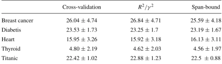
The results are shown in Table 1.
It turns out that minimizingR2/γ2or the span estimates yields approximately the same performances as picking-up the parameters which minimize the cross-validation error. This is not very surprising since cross-validation is known to be an accurate method for choosing the hyper-parameters of any learning algorithm.
A more interesting comparison is the computational cost of these methods. Table 2 shows how many SVM trainings in average are needed to select the kernel parameters on each split. The results for cross-validation are the ones reported in R¨atsch, Onoda, and
Table 1. Test error found by different algorithms for selecting the SVM parametersCandσ. Cross-validation R2/γ2 Span-bound
Breast cancer 26.04±4.74 26.84±4.71 25.59±4.18
Diabetis 23.53±1.73 23.25±1.7 23.19±1.67
Heart 15.95±3.26 15.92±3.18 16.13±3.11
Thyroid 4.80±2.19 4.62±2.03 4.56±1.97
Titanic 22.42±1.02 22.88±1.23 22.5 ±0.88
The first column reports the results from R¨atsch, Onoda, and M¨uller (2001). In the second and last column, the parameters are found by minimizingR2/γ2and the span-bound using a
gradient descent algorithm.
Table 2. Average number of SVM trainings on one training set needed to select the parametersCandσusing standard cross-validation or by minimizingR2/γ2or the span-bound.
Cross-validation R2/γ2 Span-bound
Breast cancer 500 14.2 7
Diabetis 500 12.2 9.8
Heart 500 9 6.2
Thyroid 500 3 11.6
M¨uller (2001). They tried 10 different values for C andσ and performed 5-fold cross-validation. The number of SVM trainings on each of the 5 training set needed by this method is 10×10×5=500.
The gain in complexity is impressive: on average100times fewer SVM training iterations are required to find the kernel parameters. The main reason for this gain is that there were two parameters to optimize. Because of computational reasons, exhaustive search by cross-validation can not handle the selection of more than 2 parameters, whereas our method can, as highlighted in the next section.
Discussion. As explained in Section 3.2,R2/γ2can seem to be a rough upper bound of the
span-bound, which is in an accurate estimate of the test error (Chapelle & Vapnik, 1999). However in the process of choosing the kernel parameters, what matters is to have a bound whose minimum is close to the optimal kernel parameters. Even if R2/γ2cannot be used
to estimate the test error, the previous experiments show that its minimization yields quite good results. The generalization error obtained by minimizing the span-bound (cf Table 1) are just slightly better. Since the minimization of the latter is more difficult to implement and to control (more local minima), we recommend in practice to minimizeR2/γ2. In the experiments of the following section, we will only relate experiments with this bound, but similar results have been obtained with the span-bound.
7.3. Automatic selection of scaling factors
In this experiment, we try to choose the scaling factors for an RBF and polynomial kernel of degree 2. More precisely, we consider kernels of the following form:
K(x,z)=exp
−
i
(xi−zi)2
2σ2
i
and
K(x,z)=
1+
i
xizi
σ2
i
2
Most of the experiments have been carried out on the USPS handwritten digit recognition database. This database consists of 7291 training examples and 2007 test examples of digit images of size 16×16 pixels. We try to classify digits 0 to 4 against 5 to 9. The training set has been split into 23 subsets of 317 examples and each of this subset has been used successively during the training.
To assess the feasibility of our gradient descent approach for finding kernel parameters, we first used only 16 parameters, each one corresponding to a scaling factor for a squared tile of 16 pixels as shown on figure 4.
The scaling parameters were initialized to 1. The evolution of the test error and of the bound R2/γ2is plotted versus the number of iterations in the gradient descent procedure
Figure 4. On each of the 16 tiles, the scaling factors of the 16 pixels are identical.
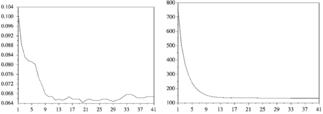
Figure 5. Evolution of the test error (left) and of the boundR2/γ2(right) during the gradient descent optimization with a polynomial kernel.
Figure 6. Evolution of the test error (left) and of the boundR2/γ2(right) during the gradient descent optimization
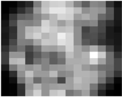
Figure 7. Scaling factors found by the optimization procedure: darker means smaller scaling factor.
Note that for the polynomial kernel, the test error went down to 9% whereas the best test error with only one scaling parameter is 9.9%. Thus, by taking several scaling parameters, we managed to make the test error decrease.
It might be interesting to have a look at the value of the scaling coefficients we have have found. For this purpose, we took 256 scaling parameters (one per pixel) and mini- mized R2/γ2with a polynomial kernel. The map of the scaling coefficient is shown in figure 7.
The result is quite consistent with what one could expect in such a situation: the coef-ficients near the border of the picture are smaller than those in the middle of the picture, so that these coefficients can be directly interpreted as measures of the relevance of the corresponding features.
Discussion. This experiment can be considered as a sanity check experiment. Indeed, it proves it is feasible to choose multiple kernel parameters of an SVM and that it does not lead to overfitting. However, the gain in test error was not our main motivation since we did not expect any significant improvement on such a problem where most features play a similar role (taking all scaling factors equal on this database seems a reasonable choice). However as highlighted by figure 7, this method can be a powerful tool to perform feature selection.
8. Feature selection
The motivation for feature selection is three-fold: 1. Improve generalization error
2. Determine the relevant features (for explanatory purposes)
3. Reduce the dimensionality of the input space (for real-time applications)
Finding optimal scaling parameters can lead to feature selection algorithms. Indeed, if one of the input components is useless for the classification problem, its scaling factor is likely to become small. But if a scaling factor becomes small enough, it means that it is possible to remove it without affecting the classification algorithm. This leads to the following idea for feature selection: keep the features whose scaling factors are the largest.
This can also be performed in a principal components space where we scale each principal component by a scaling factor.
We consider two different parametrization of the kernel. The first one correspond to rescaling the data in the input space:
Kθθθ(x,z)=K(θTx,θTz)
whereθ∈Rn
.
The second one corresponds to rescaling in the principal components space: Kθθθ(x,z)=K(θTx,θTz)
whereΣis the matrix of principal components.
We computeθandαusing the following iterative procedure:
1. Initialize θ=(1, . . . ,1)
2. In the case of principal component scaling, perform
principal component analysis to compute the matrix .
3. Solve the SVM optimization problem
4. Minimize the estimate of the error T with respect to θ
with a gradient step.
5. If a local minimum of T is not reached go to step 3.
6. Discard dimensions corresponding to small elements in θ
and return to step 2.
We demonstrate this idea on two toy problems where we show that feature selection reduces generalization error. We then apply our feature selection algorithm to DNA Micro-array data where it is important to find which genes are relevant in performing the classifica-tion. It also seems in these types of algorithms that feature selection improves performances. Lastly, we apply the algorithm to face detection and show that we can greatly reduce the input dimension without sacrificing performance.
8.1. Toy data
We compared several algorithms
• The standard SVM algorithm with no feature selection
• Our feature selection algorithm with the estimateR2/γ2and with the span estimate • The standard SVM applied after feature selection via a filter method
The three filter methods we used choose the m largest features according to: Pearson correlation coefficients, the Fisher criterion score,4and the Kolmogorov-Smirnov test.5Note
that the Pearson coefficients and Fisher criterion cannot model nonlinear dependencies. In the two following artificial datasets our objective was to assess the ability of the algorithm to select a small number of target features in the presence of irrelevant and redundant features (Weston et al., 2000).
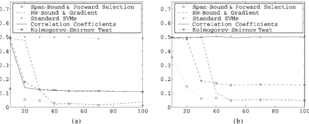
Figure 8. A comparison of feature selection methods on (a) a linear problem and (b) a nonlinear problem both with many irrelevant features. Thex-axis is the number of training points, and they-axis the test error as a fraction of test points.
For the first example, six dimensions of 202 were relevant. The probability ofy=1 or−1 was equal. The first three features{x1,x2,x3}were drawn asxi =y N(i,1)and the second
three features{x4,x5,x6}were drawn asxi =N(0,1)with a probability of 0.7, otherwise
the first three were drawn asxi =N(0,1)and the second three asxi=y N(i−3,1). The
remaining features are noisexi =N(0,20),i =7, . . . ,202.
For the second example, two dimensions of 52 were relevant. The probability ofy=1 or−1 was equal. The data are drawn from the following: ify= −1 then{x1,x2}are drawn
fromN(µ1, )orN(µ2, )with equal probability,µ1= {−3
4,−3}andµ2 = { 3 4,3}and = I, if y =1 then{x1,x2}are drawn again from two normal distributions with equal
probability, withµ1= {3,−3}andµ2= {−3,3}and the sameas before. The rest of the features are noisexi =N(0,20),i =3, . . . ,52.
In the linear problem the first six features have redundancy and the rest of the features are irrelevant. In the nonlinear problem all but the first two features are irrelevant.
We used a linear kernel for the linear problem and a second order polynomial kernel for the nonlinear problem.
We imposed the feature selection algorithms to keep only the best two features. The results are shown in figure 8 for various training set sizes, taking the average test error on 500 samples over 30 runs of each training set size. The Fisher score (not shown in graphs due to space constraints) performed almost identically to correlation coefficients.
In both problem, we clearly see that our method outperforms the other classical meth-ods for feature selection. In the nonlinear problem, among the filter methmeth-ods only the Kolmogorov-Smirnov test improved performance over standard SVMs.
8.2. DNA microarray data
Next, we tested this idea on two leukemia discrimination problems (Golub et al., 1999) and a problem of predicting treatment outcome for Medulloblastoma.6The first problem was to
classify myeloid versus lymphoblastic leukemias based on the expression of 7129 genes. The training set consists of 38 examples and the test set 34 examples. Standard linear SVMs achieve 1 error on the test set. Using gradient descent onR2/γ2we achieved 0 error using
30 genes and 1 error using 1 gene. Using the Fisher score to select features resulted in 1 error for both 1 and 30 genes.
The second leukemia classification problem was discriminating B versus T cells for lymphoblastic cells (Golub et al., 1999). Standard linear SVMs make 1 error for this problem. Using either the span bound or gradient descent onR2/γ2results in 0 error using 5 genes,
whereas the Fisher score get 2 errors using the same number of genes.
The final problem is one of predicting treatment outcome of patients that have Medulloblastoma. Here there are 60 examples each with 7129 expression values in the dataset and we use leave-one-out to measure the error rate. A standard SVM with a Gaussian kernel makes 24 errors, while selecting 60 genes using the gradient descent on R2/γ2we achieved an error of 15.
8.3. Face detection
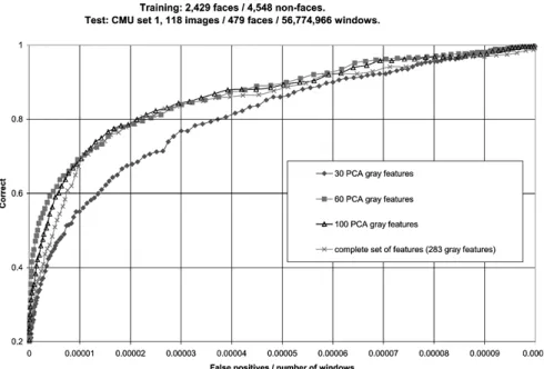
The trainable system for detecting frontal and near-frontal views of faces in gray images presented in Heisele, Poggio, and Pontil (2000) gave good results in terms of detection rates. The system used gray values of 19×19 images as inputs to a second-degree polynomial kernel SVM. This choice of kernel lead to more than 40,000 features in the feature space. Searching an image for faces at different scales took several minutes on a PC. To make
the system real-time reducing the dimensionality of the input space and the feature space was required. The feature selection in principal components space was used to reduce the dimensionality of the input space (Serre et al., 2000).
The method was evaluated on the large CMU test set 1 consisting of 479 faces and about 57,000,000 non-face patterns. In figure 9, we compare the ROC curves obtained for different numbers of selected components.
The results showed that using more than 60 components does not improve the perfor-mances of the system (Serre et al., 2000).
9. Conclusion
We proposed an approach for automatically tuning the kernel parameters of an SVM. This is based on the possibility of computing the gradient of various bounds on the generalization error with respect to these parameters. Different techniques have been proposed to smooth these bounds while preserving their accuracy in predicting the location of the minimum of test error. Using these smoothed gradients we were able to perform gradient descent to search the kernel parameter space, leading to both an improvement of the performance and a reduction of the complexity of the solution (feature selection). Using this method, we chose in the separable case appropriate scaling factors. In the non separable case, this method allows us to choose simultaneously scaling factors and parameter C (see Eq. (3)).
The benefits of this technique are many. First it allows to actually optimize a large number of parameters while previous approaches only could deal with 2 parameters at most. Even in the case of a small number of parameters, it improves the run time by a large amount. Moreover experimental results have demonstrated that an accurate estimate of the error is not required and that a simple estimate likeR2/γ2has a very good behaviour in terms of
finding the right parameters. In a way this renders the technique even more applicable since this estimate is very simple to compute and derive. Finally, this approach avoids holding out some data for validation and thus makes full use of the training set for the optimization of parameters, contrary to cross-validation methods.
This approach and the fact that it has be proven successful in various situation opens new directions of research in the theory and practice of Support Vector Machines. On the practical side, this approach makes possible the use of highly complex and tunable kernels, the tuning of scaling factors for adapting the shape of the kernel to the problem and the selection of relevant features. On the theoretical side, it demonstrates that even when a large number of parameter are simultaneously tuned the overfitting effect remains low.
Of course a lot of work remains to be done in order to properly understand the reasons. Another interesting phenomenon is the fact that the quantitative accuracy of the estimate used for the gradient descent is only marginally relevant. This raises the question of how to design good estimates for parameter tuning rather than accurate estimates.
Future investigation will focus on trying to understand these phenomena and obtain bounds on the generalization error of the overall algorithm, along with looking for new problems where this approach could be applied as well as new applications.
Acknowledgments
The authors would like to thank Jason Weston and ´Elodie N´ed´elec for helpful comments and discussions.
Notes
1. In the rest of this article, we will reference vectors and matrices using bold notation. 2. We noteP˜(x)as an abbreviation forP˜A∗,B∗(x).
3. This inequality can be easily proved by differentiating MM−1=I.
4. F(r)=µ+r−µ−r
σr++σr−
, whereµ±r is the mean value for ther-th feature in the positive and negative classes andσr±
is the standard deviation. 5. KStst(r)=
√
sup(Pˆ{X≤ fr} − ˆP{X≤ fr,yr=1}) where frdenotes ther-th feature from each training
example, andPˆis the corresponding empirical distribution.
6. The database will be available at :http://waldo.wi.mit.edu/MPR/datasets.html. References
Bengio. Y. (2000). Gradient-based optimization of hyper-parameters.Neural Computation,12:8.
Bonnans J. F. & Shapiro, A. (2000).Perturbation analysis of optimization problems. Berlin: Springer-Verlag. Chapelle, O. & Vapnik, V. (1999). Model selection for support vector machines. InAdvances in neural information
processing systems.
Cortes, C. & Vapnik, V. (1995). Support vector networks.Machine Learning,20, 273–297.
Cristianini, N., Campbell, C., & Shawe-Taylor, J. (1999). Dynamically adapting kernels in support vector machines. InAdvances in neural information processing systems.
Cristianini, N. & Shawe-Taylor, J. (2000).An introduction to support vector machines.Cambridge, MA: Cambridge University Press.
Golub, T., Slonim, D., Tamayo, P., Huard, C., Gaasenbeek, M., Mesirov, J. P., Coller, H., Loh, M. L., Downing, J. R., Caligiuri, M. A., Bloomfield, C. D., & Lander, E. S. (1999). Molecular classification of cancer: Class discovery and class prediction by gene expression monitoring.Science,286, 531–537.
Heisele, B., Poggio, T., & Pontil, M. (2000). Face detection in still gray images. AI Memo 1687, Massachusetts Institute of Technology.
Jaakkola, T. S. & Haussler, D. (1999). Probabilistic kernel regression models. InProceedings of the 1999 Confer-ence on AI and Statistics.
Joachims, T. (2000). Estimating the generalization performance of a svm efficiently. InProceedings of the Inter-national Conference on Machine Learning. San Mateo, CA: Morgan Kaufman.
Larsen, J., Svarer, C., Andersen, L. N., & Hansen, L. K. (1998). Adaptive regularization in neural network modeling. In G. B. Orr & K. R. M¨uller (Eds.).Neural networks:Trick of the trade.Berlin: Springer.
Luntz, A. & Brailovsky, V. (1969). On estimation of characters obtained in statistical procedure of recognition. Technicheskaya Kibernetica,3, (in Russian).
L¨utkepohl, H. (1996).Handbook of matrices. New York: Wiley & Sons.
Opper, M. & Winther, O. (2000). Gaussian processes and svm: Mean field and leave-one-out. In A. J. Smola, P. L. Bartlett, B. Sch¨olkopf, & D. Schuurmans (Eds.).Advances in large margin classifiers(pp. 311–326). Cambridge, MA: MIT Press.
Platt, J. (2000). Probabilities for support vector machines. In A. Smola, P. Bartlett, B. Sch¨olkopf, & D. Schuurmans (Eds.).Advances in large margin classifiers. Cambridge, MA: MIT Press.
R¨atsch, G., Onoda, T., & M¨uller, K.-R. (2001). Soft margins for AdaBoost.Machine Learning,42:3, 287–320. Serre, T., Heisele, B., Mukherjee, S., & Poggio, T. (2000). Feature selection for face detection. AI Memo 1697,
Massachusetts Institute of Technology.
Vapnik, V. (1998).Statistical learning theory. New York: John Wiley & Sons.
Vapnik, V. & Chapelle, O. (2000). Bounds on error expectation for support vector machines:Neural Computation, 12:9.
Wahba, G., Lin, Y., & Zhang, H. (2000). Generalized approximate crossvalidation for support vector machines: Another way to look at marginlike quantities. In A. Smola, P. Bartlett, B. Sch¨olkopf, & D. Schuurmans (Eds.). Advances in large margin classifiers(pp. 297–309). Cambridge, MA: MIT Press.
Weston, J., Mukherjee, S., Chapelle, O., Pontil, M., Poggio, T., & Vapnik, V. (2000). Feature selection for support vector machines. InAdvances in neural information processing systems.
Received March 14, 2000 Revised March 22, 2001 Accepted March 22, 2001 Final manuscript July 19, 2001