SOEPpapers
on Multidisciplinary Panel Data Research
So Far so Good:
Age, Happiness, and Relative Income
Felix R. FitzRoy, Michael A. Nolan, Max F. Steinhardt, David Ulph
415
2
011
SOEPpapers on Multidisciplinary Panel Data Research
at DIW Berlin
This series presents research findings based either directly on data from the German Socio-Economic Panel Study (SOEP) or using SOEP data as part of an internationally comparable data set (e.g. CNEF, ECHP, LIS, LWS, CHER/PACO). SOEP is a truly multidisciplinary household panel study covering a wide range of social and behavioral sciences: economics, sociology, psychology, survey methodology, econometrics and applied statistics, educational science, political science, public health, behavioral genetics, demography, geography, and sport science.
The decision to publish a submission in SOEPpapers is made by a board of editors chosen by the DIW Berlin to represent the wide range of disciplines covered by SOEP. There is no external referee process and papers are either accepted or rejected without revision. Papers appear in this series as works in progress and may also appear elsewhere. They often represent preliminary studies and are circulated to encourage discussion. Citation of such a paper should account for its provisional character. A revised version may be requested from the author directly.
Any opinions expressed in this series are those of the author(s) and not those of DIW Berlin. Research disseminated by DIW Berlin may include views on public policy issues, but the institute itself takes no institutional policy positions.
The SOEPpapers are available at
http://www.diw.de/soeppapers Editors:
Joachim R. Frick (Empirical Economics)
Jürgen Schupp (Sociology, Vice Dean DIW Graduate Center) Gert G. Wagner (Social Sciences)
Conchita D’Ambrosio (Public Economics)
Denis Gerstorf (Psychology, DIW Research Professor) Elke Holst (Gender Studies)
Frauke Kreuter (Survey Methodology, DIW Research Professor) Martin Kroh (Political Science and Survey Methodology)
Frieder R. Lang (Psychology, DIW Research Professor) Henning Lohmann (Sociology, DIW Research Professor)
Jörg-Peter Schräpler (Survey Methodology, DIW Research Professor) Thomas Siedler (Empirical Economics, DIW Graduate Center)
C. Katharina Spieß (Empirical Economics and Educational Science) ISSN: 1864-6689 (online)
German Socio-Economic Panel Study (SOEP) DIW Berlin
Mohrenstrasse 58 10117 Berlin, Germany
SO FAR SO GOOD:
AGE, HAPPINESS, AND RELATIVE INCOME
Felix R. FitzRoyUniversity of St. Andrews, IZA Michael A. Nolan University of Hull Max F. Steinhardt
Hamburg Institute of International Economics (HWWI), Centro Studi Luca d`Agliano
David Ulph
University of St. Andrews, SIRE
November 2011
Abstract
In a simple 2-period model of relative income under uncertainty, higher comparison income for the younger cohort can signal higher or lower expected lifetime relative income, and hence either increase or decrease well-being. With data from the German Socio-Economic Panel and the British Household Panel Survey, we first confirm the standard negative effects of comparison income on life satisfaction with all age groups, and many controls. However when we split the West German sample by age we find a positive significant effect of comparison income in the under 45s, and the usual negative effect only in the over 45 group. With the same split in UK and East German data, comparison income loses significance, which is consistent with the model prediction for the younger group. Our results provide first evidence that the standard aggregation with only a quadratic control for age can obscure major differences in the effects of relative income.
JEL classification: D10, I31, J10
Keywords: subjective life-satisfaction, comparison income, reference groups, age, welfare Acknowledgements: Earlier versions were presented at the WPEG Conference, Sheffield, July 2011, and an Economics seminar, St. Andrews, October 2011. For comments and discussion, we are grateful to Andrew Oswald, Alkis Otto, Peter Sloane, Alois Stutzer, Karl Taylor and seminar participants. The authors retain responsibility.
1. Introduction
Among the most important results in happiness research, which largely explain the Easterlin Paradox, are the negative effects of comparison or reference income, found in many different contexts (Layard et al. 2010, Clark et al. 2008, Luttmer, 2005). However as Hirschman and Rothschild (1973) observed, just before the beginning of modern research on subjective well-being by Easterlin (1974), comparison with a relevant reference group could have two very different effects. The relative income effect, which had already been discussed by a few economists, and more widely by sociologists as ‘relative deprivation’ (Runciman 1966), or status (Veblen, 1899), refers to comparison of one’s own current situation with that of the relevant reference group. However, Hirschman and Rothschild (1973) argued in the context of economic development and resulting inequality combined with rapid growth, that comparison could also indicate one’s own future prospects. Thus a higher reference income in this context might be perceived as only a temporary ‘relative deprivation’, but also as an indicator of a better future, which he denoted ‘the tunnel effect’, with an inherently ambiguous net result on current subjective well-being (SWB).
While such effects in developing countries are plausible, there is also a natural asymmetry in likely response to relative income across age groups, which has received much less attention. Young individuals everywhere are obviously more mobile and likely to see peer success as an indication of their own future prospects, (and perhaps be motivated to greater effort), than less flexible, older people. The careers of the latter group are fully determined at the latest by retirement, so expectations lose relevance and current perceptions of relative deprivation or success should dominate. This asymmetry suggests estimating the effects of relative income separately for young and old subsamples, which is our approach here, and does not seem to have been implemented previously.
First we formalise some of these ideas in a simple 2-period model with uncertainty. Depending on parameters, the young cohort finds that higher comparison income can signal either higher or lower lifetime expected relative income, and hence well-being or life satisfaction. In the second period, realised relative incomes have the usual effect. These potential differences are thus obscured by the usual aggregation of all age groups even with a quadratic in age. This is not a general model of relative income, since we do not consider optimizing responses to information and other issues, and focus on exogenous shocks to the labour market, but it does capture a novel result of the empirical analysis, namely the possibly positive (signalling) effect of higher comparison income on a young cohort’s expected well-being, an effect which is lost under the usual aggregation of age groups.
To test these ideas we use data from West Germany, East Germany, and the UK. East Germany is still (21 years after reunification) a region with high unemployment, poor career prospects for the young, (who often move west), and lower inequality than in the West, so we expect weaker effects of relative income for both the young and old samples.
Using the German Socio-economic Panel (SOEP) we estimate life-satisfaction separately for sub-samples between 18 and 45, and over 45, in both West and East, as well as for the complete samples with all ages. In West Germany with the full sample we confirm the results of Layard et al. (2010), and Ferrer-i-Carbonell (2005), who also find strong negative effects of relative income with SOEP data, using a quadratic in age and many controls. However, in contrast to all previous work that we are aware of, when we split the sample by age we actually find a positive significant effect of comparison income in West Germany for those under 45, as well as the usual negative significant effect for the older group. The absolute magnitude of the latter is larger than in the full sample, though less than the own income effect. In East Germany, relative income loses significance for all age groups, though the sign
of the coefficient remains positive for the young and negative for the old. There is also a much stronger effect of own income in the older group.
Thus a fundamental result of happiness research changes dramatically after disaggregating the complete sample, a change not captured by the usual quadratic in age: the robust negative effect of relative income turns positive in younger subsamples, a result quite consistent with Hirschman and Rothschild’s (1973) pioneering analysis, though not directly predicted by them. We next use the British Household Panel Survey, a large representative survey similar to the SOEP, to compare the effects of disaggregation in the two countries. Though the results for the whole sample are similar and quite standard, with comparison income negative and significant in the usual way, comparison income becomes insignificant for both young and old in the separate UK estimates (though the sign of the coefficient remains positive for the young and negative for the old, as in East Germany). As expected, own income is positive and significant for both groups, although its effect is stronger for the younger UK group. Estimation of well-being in samples combining young and old respondents thus generates serious bias, in two countries, in spite of controls for age, and some surprising differences in certain respects.
The plan of the paper is to provide a brief review of some more relevant literature in section 2, followed by the theoretical model in section 3. Discussion of the SOEP data, and subsequent empirical results is in section 4. Parallel discussion of the BHPS data and estimates is presented in section 5. Conclusions are summarized in section 6, and tables are in the appendix.
2. A Brief Literature Review
While Hirschman and Rothschild’s ideas have long been neglected, they were tested by Drichoutis et al. (2010), who found insignificant effects of comparison income for the
transition economies of Eastern Europe, and by Senik (2008, 2004), who found positive effects of relative income on life-satisfaction or financial satisfaction for most transition economies and Russia. She ascribes this contrast to ‘old’ Europe, with mainly negative effects of reference income, to social and economic turmoil after transition and consequent high mobility. Much less plausibly, Senik (2008) also finds a strong positive effect of relative income on happiness in the US, attributed to high perceived mobility, but this result is directly contradicted by Layard et al. (2010), using the same GSS data, and by Luttmer (2005) and others with various data sets. Senik argues that Luttmer’s neighbourhood mean income does not have the same informational content as comparison with an educational or professional peer-group, but this is questionable. Living in a more prosperous area surely also offers better career prospects than being surrounded by poverty, with lower mobility costs, as well as probably providing various local public goods, better quality services, etc., which are likely to directly raise well-being. Thus Luttmer’s (2005) negative comparison effect (for all ages) arises in spite of several potential underlying positive neighbourhood effects.
Senik (2008) includes all ages, but omits regional effects, and most seriously, both employment status and health from her second-stage explanatory variables, though these are generally found to be among the most important determinants of SWB, so their omission could cause omitted variable bias. She also uses individual income instead of the more natural household income; thus some women with little or no income may be living in affluent households, but the precise reasons for her anomalous results are unclear. Very surprisingly, Senik (2008) also reports positive significant relative income effects on financial satisfaction for Germany, Netherlands, Ireland and Spain in her Table 3, though she discusses these effects for only Ireland and Spain in the text. These results for stable western countries
are clearly contradicted by studies mentioned above – and ours below for life satisfaction.1 She claims ‘predominantly negative’ relative income effects in her sample of 14 West European countries, but reports negative significant coefficients for only 6 countries.
In a previous version of the above paper, Senik (2006) reports quite different results for financial satisfaction in the same West European countries, with highly significant, negative effects of reference income in all cases, but she does not mention these differences in the later, published version.
A different kind of test of the signalling effect of comparison income has been carried out by Clark et al. (2009), using Danish establishment wage data, with the plausible finding that job-satisfaction is higher in establishments with higher average pay, which plausibly signals one’s own prospects. Interestingly in the light of our findings below, they find less effect for those near retirement. However, it is also likely that higher average pay will be correlated with work-place public goods as part of rent-sharing with workers, which may explain part of the observed influence.
By contrast, in an early study with UK data for employees, Clark and Oswald (1996) found a strong negative effect of reference income on job-satisfaction (which is generally an important component of life-satisfaction), equal in magnitude and opposite in sign to the own-income effect. Card et al (2011) find a negative effect of higher comparison income on job-satisfaction, when this information is first revealed. There is also evidence for the importance of comparison from neuroscience (Fliessbach et al, 2007). Separating sub-samples of young and old does not seem to have been considered previously.2
1
Senik (2008) uses ‘jealousy’ in her title and text, to refer to the relative deprivation effect of comparison, (sometimes interpreted as preference for fairness, or as envy). In fact, jealousy refers to ‘an anticipated loss’ and ‘is not to be confused with envy’ (Wikipedia).
2
Senik (2008) uses an age-interaction term to find stronger positive effects of reference income for younger respondents in Eastern Europe, and in the US, but reports no evidence of negative comparison effects for older individuals.
3. Happiness over the life cycle
Theory
In this section we set out a model that supports our empirical findings – specifically the finding that, in the early stages of working life, the average income of the comparison group may have either a positive or insignificant effect on reported happiness or life-satisfaction3. The essential insight we wish to capture is that life-satisfaction may depend on not just a comparison of a person’s own current income with the current income of their peers, but also on a comparison of how their life as a whole is going relative to their peers, and so on relative life-time income. Of course early in their working life people do not know for sure how their lives might pan out and, in particular, how not just their own life-time income but that of the comparison group will evolve. So they use information about how their life has gone to date – specifically their current income and that of their peers – to draw inferences about how things might go in the future. In this context a high current income of the comparison group may signal that there has been a significant amount of promotion to date and hence future promotion prospects and so expectations of relative future life-time income are good.
The aim of the model is to formalise this idea and show that there are indeed contexts in which, in the earlier part of working life, the current income of the comparison group may be positively associated with reported happiness.
The Model
The model is framed in a way that is consistent with the data on which the empirical analysis has been conducted. So it is assumed that individuals’ working lives are split into two periods.
We also assume that all individuals have a comparison/peer group with whom they compare how their lives are going. Accordingly we consider a sub-population of individuals who are
3
As noted, this contrasts with the well-established finding – which we also report – that, when all age groups are pooled together, average income of the comparison group has a significant negative impact on reported happiness or life-satisfaction.
identical in terms of some observable characteristics: age, educational attainment, location etc. This constitutes the comparison/peer group to which everyone within the sub-population compares themselves.
Though identical in certain respects, individuals differ in some other characteristics that are unobservable to them but will manifest themselves over the course of their lifetime in two different respects:
Individuals may turn out to be Hares or Tortoises. Hares show early promise and get promoted early (in period 1). Tortoises develop more slowly, and get promoted, if at all, later in life – in period 2. Individuals learn in period 1 whether or not they have been promoted and hence whether they are Hares or Tortoises. So in period 1 the current income of a Tortoise is 1T
c b where b > 0 denotes basic income, while the current income of a Hare is c1H b(1) where 0 is the proportionate income supplement obtained through promotion in Period 1.
Individuals may turn out to be genuinely Smart or basically Dull. Smartness only manifests itself in period 2, and leads to Smart people – Tortoises or Hares – being promoted (further promoted) in Period 2. It is assumed that Smart Tortoises turn out to equally smart as Smart Hares and so, in period 2, their current incomes are
2 2 (1 )
ST SH
c c b where 0 represents a smartness factor – the extent to which promoted people get an extra income supplement to reflect the value of real smartness rather than the flashiness of a Hare. In Period 2 some of the Hares who were promoted in period 1 will turn out not to actually have much substance and will be Dull Hares. Having already been promoted they tread water in terms of income and so in period 2 get current income c2DH b(1). Finally Dull Tortoises don’t get promoted in period 2 either and so end up with current income 2DT
For simplicity it is assumed that these two manifested characteristics – flashiness and smartness – are independently distributed in the population. Let pH, 0 pH 1 be the proportion of people who are Hares, and pS, 0 pS 1 be the proportion of people who are Smart.
In period 1 the average current income of the group is
1 H 1H 1 H 1T (1 H ) c p c p c b p , while in period 2 it is
2 1 S 1 S H 1 S 1 H
c b p p p c p b p
It is assumed that the happiness experienced by each person in each period depends on i. A comparison of their current income with the average current income of their peers. ii. A comparison of their view of their life-time income with the average life-time
income of their peers. In period 1 life-time income is not fully known so individuals have to estimate both their own life-time income and the average life-time income of their peers.
It follows from the above assumptions that, at the end of Period 1:
the expected lifetime income of a Hare is
1 2 1
eH H
S
y c p b
the expected lifetime income of a Tortoise is
1 2 1
eT T
S
y c p b
the expected average lifetime income of the peer group is
1
1 2 S 1 H
y c p b p .
Now suppose that although, for individuals, the probability of being Smart is the same whether or not they are a Hare or a Tortoise, nevertheless in the population as a whole, the proportion of Smart people is related to the proportion of Hares by
S H
p p 4 (1)
It follows from this that, at the end of Period 1:
the expected lifetime income of a Hare is
1 2 1
eH H
H
y c p b (2)
the expected lifetime income of a Tortoise is
1 2 1
eT T
H
y c p b (3)
the expected average lifetime income of the peer group is
21
1 2 H H
y c p b p b
b
. (4)
Information structure
The information structure of the model is as follows.
At the outset, and throughout their lives, individuals know: the values of and - the income premiums to flashiness and smartness respectively; the relationship between period 1 and period 2 incomes conditional on being of various types; and the relationship between pS and pH as given by (1).
However initially they do not know the economic prospects for their cohort – whether they have skills that will turn out to be in high demand and lead to high opportunities for promotion. That is, initially they do not know the values of b and pH.
However in Period 1 they learn their own income and that of their peers, and so, by comparing them, they know whether they have turned out be a Hare or a Tortoise. Formally, they learn c1j, jH T, ; the average income of their peers, c1; their
4
We could make the more general assumption that S H, 0 1
H
p p
p
, but that adds very little to the analysis.
current income relative to that of their peers, 1 1
1
, ,
j
crj c j H T
c
and hence their
type H or T. Also from what they learn in Period 1 they can deduce the values of b
and pH and hence, from (1), the value of their future promotion prospects, pS. Using this they can use (2), (3) and (4) to calculate their own expected lifetime income and the average of that of their peers.
In period 2 everything is revealed. Individuals learn the value of their current income in period 2 and the average current income of their peers. Comparing their current income in period 2 to that earned in period 1, they learn whether they are Smart or Dull, so they now fully know their type. They can now carry out a full comparison of how their life has gone relative to their peers in terms of both their relative current income and their relative lifetime income. Formally individuals learn their period two income c2jk, jS D, ; k H T, and hence their type jk, jS D, ; k H T, . They also learn the average period 2 income of their peers c2.5 Individuals therefore
know their full life-time income y2jk c1k c2jk, jS D k, ; H T, and the average life-time income of their peers: y2 c1 c2.
Implications
Having set out the assumptions of the model, we now derive the implications. The fundamental issue we want to investigate is how the average current income of the peer group in each of the two periods affects each individual’s reported happiness, taking as given their own income. In particular we want to explore the possibility that, although a higher level of peer income in Period 1 lowers relative current income, it might raise expected relative
lifetime income, since it sends a signal about higher promotion prospects in the future.
5
Unfolding Lives Period 1
Hares
In period 1 Hares learn their current income c1H b(1) and the average income of their peers, c1 b(1 pH). Hence they know their relative current period 1 income
1 1
1
1
H
c H c
r c
which is, of course, a strictly decreasing function of the average period 1 income of their peers.
From this they calculate:
1
1 ; (1 ) 1
1 (1 )
H H
H
c c c
b bp
(5)
Substitute (5) into (2) and (4) to get:
1
1 1
1
2 (1 ) (1 ) (1 )
H H
eH c c c
y
(6)
21 1 1 1 1
1 1
1
2 (1 ) (1 ) (1 )
(1 )
H H
H H
c c c c c
c y
(7)
where y1H is the average lifetime income that Hares expect their peers to get on the basis of the information available to Hares in Period 1.
It is straightforward to show that
1 1
1 1
( ) 2 1
0 H eH H p y y c c
(8)
so, other things being equal, the higher is the current income of their peers, the higher is the realised proportion of Hares in the population, and so, from (1), the greater the promotion
prospects they face in Period 2. This raises Hares’ estimated value of their own life-time income, but also that of their peers, and indeed the latter increases by more than the former. Now from (6) and (7), in Period 1 Hares expect to end up with a relative lifetime income:
1 1 1 1 1 1 21 1 1 1 1
1
2 (1 ) (1 )
1 2 (1 ) (1 ) (1 )
eH y eH H H H H H H y r y
c c c
c c c c c
c (9)
It is straightforward to show that
1 2
2(1 )
1 2(1 ) 1 1
y eH H
H H H
p r
p p p
(10)
and so, as we know must be the case, the expected life-time income of Hares is greater than the expected lifetime income of their peers.
By differentiating (9) w.r.t c1 we get:
1 1
1
1 1 1
1 1 H eH y eH y eH H y y r
r c c
c y
(11)
which, from (8) and (10) is strictly negative, so the relative lifetime income expected by Hares in period 1 is a decreasing function of average current income of their peers, and so too is their happiness.
Tortoises
In period 1 Tortoises learn their current income 1T
c b and the average income of their peers,
1 (1 H )
c b p . Hence they know their relative current period 1 income
1 1
1
1
T
c T c
r c
(12)
which is, of course, a strictly decreasing function of the average period 1 income of their peers.
From this information Tortoises can also work out: 1 1 1; T T H c c b c bp
(13)
Substitute (13) into (3) and (4) to get:
1
1 1
1
2 T T
eT c c c
y
(14)
21 1 1 1 1
1 1
1
2 T T T
T
c c c c c
c y
(15)
where y1T is the average lifetime income that Tortoises expect their peers to get on the basis of the information available to Tortoises in Period 1.
It is straightforward to show that
1 1
1 1
( ) 2 1
0 T eT H p y y c c
(16)
so, just as with Hares, the higher is the current income of their peers, the higher is the realised proportion of Hares in the population, and so, from (1), the greater the promotion prospects that Tortoises face in Period 2. This raises Tortoises’ estimated value of their own life-time income, but also that of their peers, and indeed the latter increases by more than the former. Now from (14) and (15), in Period 1 Tortoises expect to end up with a relative lifetime income:
1 1 1 1 1 21 1 1 1 1 1
1
2 ( )
1 2 T T eT y eT T T T T
c c c
y r
y c c c c c
c (17)
It is straightforward to show that
1
2 ( )
1
2 2
y eT H
H H H
p r
p p p
and so, as we know must be the case, the expected life-time income of Tortoises is lower than the expected lifetime income of their peers.
By differentiating (18) w.r.t c1 we get:
1 1
1
1 1 1
1 1 T eT y eT y eT T y y r
r c c
c y
(19)
Consequently 1 1 1 1 1 1 1 0 eT y eT y eT T y r c r c y c (20)
Substitute (16) into (20) and we get:
1 1
2 ( ) 0
( ) 2 1 2 2
y eT
H
H H H H
r p
p p p p
c
(21)
It is clear that if pH 0 then 1 1 0 y eT r c
, whereas if pH 1 then
1 1 0 y eT r c
, so the conclusion
is that if pH is sufficiently large then an increase in the average income earned by their peers in Period 1 raises the expected relative lifetime income of Tortoises and so, potentially their happiness.
Period Two
This is straightforward.
Each type of individual knows their current period 2 income, c2jk, jS D, ; k H T, and the average period 2 income of their peers c2. Consequently they can work out their relative
current income 2 2 2 , ; , jk
c jk c
r j S D k H T
c
Each individual also sees clearly their relative performance in terms of life-time income
2 1 2
2
1 2 2
, ; ,
jk k jk
y jk y c c
r j S D k H T
y c c
and this too is a strictly decreasing function of the average period 2 income of their peers c2.
So, unambiguously, happiness of all individuals is a strictly decreasing function of the average period 2 income of their peers c2.
Conclusion
Though very simple this model seems to be capable of generating predictions that are consistent with the empirical evidence, namely that, under some circumstances and for some individuals an increase in the average current income earned by their peers may make people happier early in life, because of the signalling role it plays on prospects for future relative lifetime income. However later in life when everything has been learned, then, ceteris paribus, the higher the current income of their peers the worse people think they have performed in relative terms whether this is viewed in terms of just current performance or, looking back over one’s life, in terms of lifetime performance.
4. Empirical Evidence from the German SOEP
The data used for this section comes from the German Socio-Economic Panel (SOEP), which is a representative micro data set providing detailed information on persons, families and households in Germany (Wagner, et al 2007). The SOEP was started in 1984 and has become a widely used database for sociologists and economists. A major advantage is the comprehensive nature of the data set, which combines objective indicators (e.g. income, employment status, family structure), as well as subjective or self-assessed life-satisfaction. In our paper, we make use of the entire 2008 wave of the SOEP after excluding retired
individuals6, and analyse the nexus between happiness, relative income and age based on 9,725 individual observations.
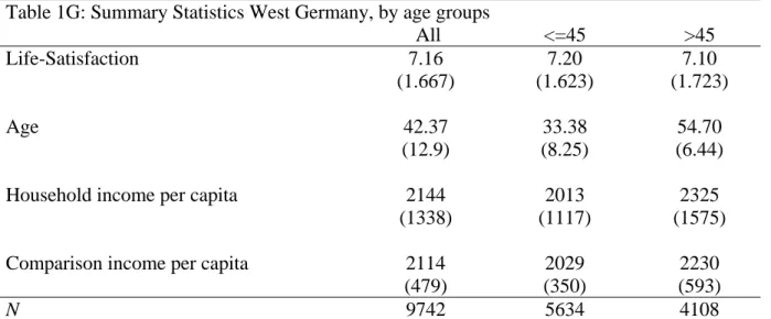
Our dependent variable is an individual’s self-reported life-satisfaction which is measured on an 11 point scale, 0 being the lowest value, while 10 is reported by individuals who are very satisfied with their actual life. Our main explanatory variables of interest are individual and reference income, which are both measured at the household level after deducting taxes and social insurance contributions.7 We also report the usual quadratic in age (Blanchflower and Oswald, 2008). For the identification of the comparison or reference income, we follow Layard et al. (2010) and assume that an individual compares his/her own income with the average income of people in his/her own country, who are in the same age range, have the same gender and have attained a similar education level. We therefore define an individual’s reference group by his/ her age (6 categories), education (2 categories) and gender. Experiments with different definitions of comparison income show that results are robust. Additionally, we distinguish between the place of residence of an individual (West vs. East Germany). Moreover, we present our analysis separately for East and West Germany. This is motivated by large and persisting socio-economic and cultural differences between both regions, which are highlighted in tables 1G and 2G. The tables provide summary statistics and detailed definitions of our dependent and main explanatory variables described above. We see that individuals in East Germany are on average less satisfied with their life than those living in West Germany. This corresponds to the fact, that East Germans are more affected by unemployment and have significantly lower household income then West Germans. Due to the construction of the variable, the latter also holds true for reference income. The well-known regional disparities in employment and income between West and
6
Results remain very similar if we include retired individuals. Either way, the proportion of females in the sample stays much the same (perhaps a little surprisingly).
7
We adjust for the number of adults in the household, though this makes little difference to the results. In cases with 2 adults, we divide household income by 1.6. In cases of three or more adults within a household, we use a divisor of 2.1.
East Germany are therefore clearly reflected in our data. However, the average life-satisfaction score in East Germany is still about 6.7, which is fairly high compared to self-reported happiness in the US (Layard et al. 2010). The tables also contain summary statistics of our dependent and independent variables broken down by age groups. It becomes obvious that the differences in happiness and economic outcomes between West and East Germany hold true when we compare people within age groups. Finally, the tables show that young adults in East and West Germany are on average more satisfied with their life than older individuals.
To test the influence of reference income on life-satisfaction we estimate the following model:
, (22)
where H measures self-reported life-satisfaction on an 11-point scale, and X is a vector of individual covariates including individual characteristics like gender, employment status and self-reported health as well as dummies for federal states. Y captures annual net household income of an individual, while Y describes the mean income of the corresponding reference group defined by age, gender, education and region.
Column (1) of table 3G reports the results of our benchmark specification for West Germany. Our positive and significant income coefficient has a similar size as the one found by Layard et al. (2010) who exploit the panel aspect of the SOEP and use individual fixed effects. 8 With respect to the role of relative income, we confirm the recent findings of Layard et al. (2010), Luttmer (2005), Ferrer-i-Carbonell (2005) and others: reference income has a negative effect on individual well -being. However, the positive influence of own income is still larger than the negative effect of reference income.
8
However, they exclude immigrants and individuals under 30 and over 55. Due to the cross-sectional nature of the data used, we do not control for unobserved heterogeneity of the respondents. Layard et al (2010) find that individual fixed effects preserve a highly significant, negative reference income effect, nearly as large in magnitude as the own income effect.
Using many controls provides higher explanatory power of our estimates than is usual in cross-sectional regressions. For data reasons we do not use the full panel with individual fixed effects, but Layard et al. (2010) show that fixed effects only reduce the size of the coefficients of own-income and relative income (and some controls), but do not change signs or statistical significance of the income variables. They also show that adaptation provides only small additional explanatory power in the SOEP.
By estimating a simple OLS model, we treat life-satisfaction scores as cardinal and comparable across respondents. This assumption is sometimes criticised in the economic literature, but estimates from an ordered probit model are qualitatively similar to the ones reported in table 3G. This is in line with the findings of Ferrer-i-Carbonell and Frijters (2004) who demonstrate that the assumptions on cardinality or ordinality of answers to life-satisfaction questions have no substantial impact on the empirical results. The other individual factors and control variables influence individual life-satisfaction in the usual way: e.g. being married is positively associated with individual well-being, as is health and work status.
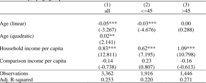
The results for East Germany are presented in table 4G. As expected, the income coefficients have a larger magnitude than for West Germany. In regions that are characterized by low income and high unemployment levels, own income has a higher relevance for individual well-being. In addition to this, the results indicate that reference income does not matter for individuals in East Germany, neither in the full sample nor in either age group. For the younger group this is consistent with our model, and may be related to less inequality, and to the fact that the best career opportunities for young adults in the East are widely perceived to result from moving to the West. Similar results are found by Drichoutis et al. (2010) for East European transition economies, though without separating by age. For the older group one might think of lower income inequality as a reason for no comparison effect, but then we find
the same insignificance of comparison income for older respondents in the much more unequal UK, which is more surprising.
Table 3G also provides estimates for West Germany stratified by age groups. The results in column (2) highlight that reference income has a positive significant effect for individuals not older than 45. The standard negative relationship between reference income and individual well-being only holds true for individuals older than 45 (see column 3).9 Thus a fundamental result of happiness research changes dramatically as soon as we disaggregate the sample into young and old individuals. Our findings are consistent with the model prediction that the positive signalling effect can dominate the negative deprivation effect for young adults: during early career phases with high job and income mobility, comparison income helps to predict own future earnings and therefore impacts positively upon own satisfaction. Only when an individual has reached a stable position within his/her career, does comparison with reference income signal lasting positive status or relative deprivation in the usual manner, so that higher comparison income reduces corresponding well-being. The quadratic age effect in the full sample is captured by linear effects, negative for the younger and positive for the older. While obviously important, these standard age effects clearly do not expose the striking differences in response to relative income which are revealed by separate estimates for the two age groups, as we also find in the following results for the UK.
5. Empirical Evidence from the BHPS
Our UK data are taken from the Wave 17 of the British Household Panel Survey, (BHPS), which is also for 2008. We use data for 9599 observations after retired individuals and
9
Our results are qualitatively similar if we change the age limits for the two subsamples.
missing values are excluded10. One point worthy of note is the deliberate over-sampling of the smaller nations of the UK – so that about half of the individuals in the BHPS are from Scotland, Wales and Northern Ireland, compared to less than 20% in the underlying overall population. While there are differences compared to England, they are much less than between West and East Germany, so do not warrant separate estimates. The range of coverage of this data set is similarly broad as the SOEP, although unsurprisingly not identical. For example, self-reported life-satisfaction is measured on a scale from 1-7. The average life-satisfaction, at just below 5.2, would equate to just below 7.0 on the 0-10 scale (if a linear translation were used) – a little below the mean for West Germany from the SOEP11. The income variable used from the BHPS data is household income for the month before the survey interview. For reference income, we identify reference groups by the same number of age and education bands – as well as separating by gender and splitting England from non-England. For individuals who are married or cohabiting, household income is divided by 1.6.
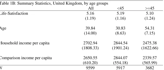
The methodology parallels our analysis of the SOEP data above, and the corresponding tables of results are in Appendix B. Summary statistics, overall and for the two sub-samples, are presented in table 1B. The benchmark regression across all ages, and separate estimates for younger and older individuals, are reported in table 3B. Despite the similarities between the surveys, and many of the standard control effects, there are some striking differences between the two countries, some of which really only become apparent after disaggregation. Whereas mean household income is higher for older workers in the SOEP data (by 15% for West
10
Results are similar if we exclude those over 60. However, in contrast to the SOEP sample, the oldest or retired group does respond differently to those still working, possibly because assets are more important in the UK, where pensions are less generous, but in any case this is beyond our scope here. As with the SOEP data, the gender split remains little altered by the exclusion of retired people.
11
The averages for Wales and Scotland are almost identical, just below the UK average, while that for England is fractionally above. Northern Ireland is a bit different, averaging a little over 5.2 (but is still not equivalent to West Germany).
Germany and 4% for East Germany), older (non-retired) members of the BHPS sample suffer an average deficit of roughly 13%.
While income variables are significant with expected signs in the overall estimates, only own income remains significant after splitting the sample. Remarkably, the own-income coefficients are much smaller than the corresponding coefficients for SOEP (even taking into account the lesser range across which life-satisfaction is measured in the BHPS), and smaller for the older group than for the younger. In both West and East Germany the coefficients for the older are about twice the size of those for the younger. This is in the spirit of our model, where expectations should be more important for the younger. The absence of a significant effect of reference income in the younger sub-sample is consistent with the model, but it remains puzzling that the significant negative relative income effect in the full sample becomes insignificant in the older sub-sample, as in very different East Germany. Exploiting the panel data and including individual fixed effects typically reduces the size and significance of existing coefficients, and thus seems unlikely to generate a negative and significant relative income effect in the older group. In any case, various results only become apparent after splitting the sample by age, and reveal several open questions for future research.
6. Conclusions
While the results from the entire sample for West Germany confirm previous findings that reference income has a strong negative effect on well-being, our sub-sample regressions for different age groups show that the effect of comparison income on individual life-satisfaction changes dramatically over the life-cycle, reversing sign, while increasing in magnitude. This confirmation of our model prediction (and of Hirschman’s ‘tunnel hypothesis’ in the unexpected context of a stable, advanced economy with relatively low mobility) clearly has
major consequences for the interpretation of well-being, comparison, and relative optimism or deprivation over the life-cycle. Aggregation over ages and relying on a quadratic in age obscures major differences in the role of relative incomes. We are not aware of any other such results in the literature on happiness and relative income.
For the UK we find a different result after disaggregating by age. The conventional reference income effects in the whole sample disappear for both age groups. Aggregating over age groups and relying on a quadratic in age has obscured this surprising result, which contrasts with our German estimates. Life-satisfaction and other measures of well-being clearly need to be estimated separately for young and old in future research, and the role of expectations, mobility and inequality seem worth exploring for their relevance to well-being and social comparison.
Going beyond our cross-sectional focus here, these results may perhaps also provide an additional explanation for the observed trends in happiness in industrialized/developed countries. Due to ageing populations, and shrinking shares of young people (who are likely to experience gains in SWB from increasing reference income and economic growth), average happiness is more likely to stagnate.
References
Blanchflower, D. G., Oswald, A., 2008. Is well-being U-shaped over the life cycle? Social Science & Medicine 66, 1733 – 1749.
Clark, A. E., Frijters, P., Shields, M. A., 2008. Relative income, happiness, and utility: An explanation for the Easterlin paradox and other puzzles. Journal of Economic Literature 46, 95-144.
Clark, A. E., Kristensen, N., Westergård-Nielsen, N., 2009. Job Satisfaction and Co-worker Wages: Status or Signal? Economic Journal 119, 430 – 447.
Clark, A. E., Oswald, A., 1996. Satisfaction and comparison income. Journal of Public Economics 61, 359 – 381.
Card, D., Mas, A., Moretti, E., Saez, E., 2011. Inequality at Work: The Effect of Peer Salaries on Job Satisfaction. NBER Working Paper No. 16396
Drichoutis, A. C., Nayga , R. M., Lazaridis, P., 2010. Do reference values matter? Some notes and extensions on income and happiness across Europe. Journal of Economic Psychology 31, 479 – 486.
Easterlin, R., 1974. Does Economic Growth Improve the Human Lot? In: David, P.A., Reder, M.W. (Eds.), Nations and Households in Economic Growth: Essays in Honour of Moses Abramowitz.Academic Press, New York, pp. 89–125.
Ferrer-i-Carbonell, A., P. Frijters, 2004. How important is methodology for the estimates of the determinants of happiness. The Economic Journal, 114 (July), pp: 641–659.
Ferrer-i-Carbonell, A., 2005. Income and well-being: an empirical analysis of the comparison income effect. Journal of Public Economics 89, 997-1019.
Fliessbach, K., Weber, B., Trautner, P., Dohmen, T., Sunde, U., Elger, C., and Falk, A. (2007). “Social comparison affects reward-related brain activity in the human ventral striatum," Science 318, 1305-1308.
Hirschman, A. O., M. Rothschild, 1973. The Changing Tolerance for Income Inequality in the Course of Economic Development.The Quarterly Journal of Economics87, 544 – 566. Koecher, R., Raffelhueschen, B., 2011. Gluecksatlas Deutschland 2011. Deutsche Post.
Layard, R., Mayraz, G., Nickell, S., 2010. Does Relative Income Matter? Are the Critics Right? Chapter 6. In: Diener, E., Helliwell, J. F., Kahneman, D., (Eds.), International Differences in Well-being,Oxford University Press.
Luttmer, R. F. P., 2005. Neighbors as Negatives: Relative Earnings and Well-Being. Quarterly Journal of Economics 30, 963-1002.
Runciman, W. G., 1966. Relative Deprivation and Social Justice. Routledge and Kegan Paul, London.
Senik, C., 2004. When Information Dominates Comparison: Learning from Russian Subjective Panel Data. Journal of Public Economics 88, 2099–2133.
Senik, C., 2006. Ambition and Jealousy: Income Interactions in the ‘Old’ Europe versus the ‘New’ Europe and the United States. IZA Discussion PaperNo. 2083.
Senik, C., 2008. Ambition and Jealousy: Income Interactions in the ‘Old’ Europe versus the ‘New’ Europe and the United States. Economica 75, 495–513.
Veblen, T. 1899. The Theory of the Leisure Class. Macmillan Company, New York.
Wagner, G. G., Frick, J.R., and Schupp, J., 2007. The German Socio-Economic Panel Study (SOEP) - Scope, Evolution and Enhancements. Schmollers Jahrbuch 127, no. 1, 139-169.
Appendix G –SOEP Results Tables
Table 1G: Summary Statistics West Germany, by age groups
All <=45 >45
Life-Satisfaction 7.16 7.20 7.10
(1.667) (1.623) (1.723)
Age 42.37 33.38 54.70
(12.9) (8.25) (6.44)
Household income per capita 2144 2013 2325
(1338) (1117) (1575)
Comparison income per capita 2114 2029 2230
(479) (350) (593)
N 9742 5634 4108
Mean coefficients; standard deviations in parentheses. Life-Satisfaction measures self-reported life-satisfaction on an 11-point scale. Age describes the age of the respondent. Household income per capita measures the net monthly household income of the respondent adjusted by the people of adults in the household. Comparison income per capita measures the average net monthly adjusted household income within the skill group (Age (6 categories), Sex, Education (2 categories), Region (East vs. West)) to which the respondent belongs. Source: SOEP 2008
Table 2G: Summary Statistics East Germany, by age groups
All <=45 >45
Life-Satisfaction 6.72 6.91 6.48
(1.71) (1.60) (1.82)
Age 41.45 32.11 53.83
(12.98) (8.33) (5.57)
Household income per capita 1676 1649 1712
(908) (833) (998)
Comparison income per capita 1652 1640 1667
(315) (258) (377)
N 3362 1916 1446
Mean coefficients; standard deviations in parentheses. See end of Table 1 for a definition of the variables. Source: SOEP 2008
Table 3G: Life Satisfaction, West Germany, by age groups
(1) (2) (3)
all <=45 >45
Age (linear) -0.05*** -0.01*** 0.02***
(-5.735) (-4.112) (5.058)
Age (quadratic) 0.03***
(6.124)
Household income per capita 0.41*** 0.27*** 0.59***
(11.039) (5.389) (10.498)
Comparison income per capita -0.31*** 0.34** -0.68***
(-3.215) (2.291) (-4.994)
Observations 9,742 5,634 4,108
Adj. R-squared 0.218 0.202 0.243
Results from OLS regressions. Dependent variable: Life-Satisfaction. Controls for gender, marriage, cohabiting, children, health status, foreign-born, social activities, higher education, work status, interview form and federal states are included. The quadratic age regressors are divided by 50 to assist in yielding reasonable scaling of attached estimates. Robust t-statistics in parentheses. *** p<0.01, ** p<0.05, * p<0.1
Table 4G: Life Satisfaction, East Germany, by age groups
(1) (2) (3)
all <=45 >45
Age (linear) -0.05*** -0.03*** 0.00
(-3.267) (-4.676) (0.288)
Age (quadratic) 0.02**
(2.141)
Household income per capita 0.83*** 0.62*** 1.09***
(12.811) (7.195) (10.798)
Comparison income per capita -0.14 0.23 -0.16
(-0.738) (0.807) (-0.613)
Observations 3,362 1,916 1,446
Adj. R-squared 0.253 0.220 0.271
Results from OLS regressions. Dependent variable: Life-Satisfaction. For an overview of the controls included see end of table 3.Robust t-statistics in parentheses. *** p<0.01, ** p<0.05, * p<0.1
Appendix B – BHPS Tables
Table 1B: Summary Statistics, United Kingdom, by age groups
All <45 >=45
Life-Satisfaction 5.16 5.19 5.10
(1.19) (1.16) (1.24)
Age 39.84 30.83 54.31
(14.00) (8.63) (7.15)
Household income per capita 2702.94 2844.54 2475.38
(1808.33) (1901.24) (1622.66)
Comparison income per capita 2650.55 2844.07 2339.57
(610.20) (554.18) (565.99)
N 9599 5917 3682
Mean coefficients; standard deviations in parentheses. Life-Satisfaction measures self-reported life-satisfaction on a 7-point scale. Age refers to the age of the respondent. Household income per capita is the household income of the respondent in the month prior to interview, adjusted according to the respondent’s marital status. Comparison income per capita measures the average monthly adjusted household income within the skill group (Age (6 categories), Sex, Education (2 categories), Region (England vs. non-England)) to which the respondent belongs. Source: BHPS, Wave 17, 2008.
Table 2B: United Kingdom, by age groups
(1) (2) (3)
all <45 >=45
Age (linear) -0.063*** -0.012*** 0.026***
(-11.11) (-4.29) (5.07)
Age (quadratic) 0.035***
(10.70)
Household income per capita 0.095*** 0.116*** 0.071**
(5.34) (5.09) (2.46)
Comparison income per capita -0.234** 0.116 -0.088
(-2.44) (0.88) (-0.44)
Observations 9599 5917 3682
Adj. R-squared 0.174 0.157 0.206
Results from OLS regressions. Dependent variable: Life-Satisfaction. Controls for gender, marriage, cohabiting, children, health status, social activities, education, work status, and Government Office Region are included. The quadratic age regressors are divided by 50 to assist in yielding reasonable scaling of attached estimates. Robust t-statistics are in parentheses. *** denotes p-value < 0.01, ** denotes p < 0.05, * denotes p < 0.1.