Widely Linear State Space Filtering of Improper Complex Signals

(1)

Widely Linear State Space Filtering

of

Improper Complex Signals

by

Dahir H. Dini MEng(Hons)

PhD Thesis

Communications and Signal Processing Research Group Department of Electrical and Electronic Engineering

Imperial College London 2013

(2)

Copyright

The copyright of this thesis rests with the author and is made available under a Creative Commons Attribution Non-Commercial No Derivatives licence. Researchers are free to copy, distribute or transmit the thesis on the condition that they attribute it, that they do not use it for commercial purposes and that they do not alter, transform or build upon it. For any reuse or redistribution, researchers must make clear to others the licence terms of this work.

(3)

3

Abstract

Complex signals are the backbone of many modern applications, such as power systems, communication systems, biomedical sciences and military technologies. However, standard complex valued signal processing approaches are suited to only a subset of complex signals known as proper, and are inadequate of the generality of complex signals, as they do not fully exploit the available information. This is mainly due to the inherent blindness of the algorithms to the complete second order statistics of the signals, or due to under-modelling of the underlying system. The aim of this thesis is to provide enhanced complex valued, state space based, signal processing solutions for the generality of complex signals and systems.

This is achieved based on the recent advances in the so called augmented com-plex statistics and widely linear modelling, which have brought to light the limitations of conventional statistical complex signal processing approaches. Exploiting these devel-opments, we propose a class of widely linear adaptive state space estimation techniques, which provide a unified framework and enhanced performance for the generality of complex signals, compared with conventional approaches. These include the linear and nonlinear Kalman and particle filters, whereby it is shown that catering for the complete second or-der information and system models leads to significant performance gains. The proposed techniques are also extended to the case of cooperative distributed estimation, where nodes in a network collaborate locally to estimate signals, under a framework that caters for general complex signals, as well as the cross-correlations between observation noises, unlike earlier solutions. The analysis of the algorithms are supported by numerous case studies, including frequency estimation in three phase power systems, DIFAR sonobuoy underwater target tracking, and real-world wind modeling and prediction.

(4)

Acknowledgment

I would like to thank everyone who helped and supported me during my time at Impe-rial. In particular I would like to express my gratitude to Prof. Danilo Mandic for his supervision, technical support, and unflagging enthusiasm.

This work has also benefited greatly from the advice and discussions I have had over the years with many close friends. I would also like to thank my friends who have made my experiences inside and outside Imperial interesting and memorable.

I would like to reserve my biggest gratitude for my family, and thank them for their guidance and support.

This research was part of the University Defence Research Centre (UDRC) at Im-perial College London, sponsored by the MoD and DSTL (Project Code: C3).

(5)

5

List of Figures

2.1 An illustration of the importance of phase in pictures. The Figures (a) and (b) are the original images, while figure (c) consists of the magnitude information from (a) and the phase information from (b), and vice versa for Figure (d). The visual perceptions of (c) and (d) are largely dominated by the phase information. . . 28 2.2 A geometric view of circularity via a real-imaginary scatter plot of zero-mean complex white

Gaussian distributions. . . 30 2.3 A real-imaginary scatter plot of zero-mean complex white uniform distributions with zero

pseudocovariances (both are proper). . . 31 2.4 A geometric view of circularity via a real-imaginary scatter plot of white complex Gaussian

processes at different degrees of noncircularity (η), with orthogonal real and imaginary parts. 40

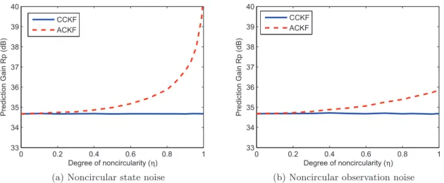
3.1 Performance of the complex UT and augmented complex UT . . . 64 3.2 Steady-state performance comparison between CCKF and ACKF for the AR(1) filtering

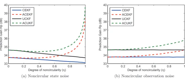
problem: (a) circular observation noise and a noncircular state noise with varying degrees of noncircularity; (b) circular state noise and noncircular observation noise with varying degrees of noncircularity. . . 69 3.3 Steady-state performance comparison between CEKF, CUKF and their corresponding

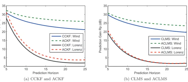
widely linear (augmented) versions for the AR(1) filtering problem: (a) circular observa-tion noise and a noncircular state noise with varying degrees of noncircularity; (b) circular state noise and noncircular observation noise with varying degrees of noncircularity. . . 70 3.4 Multistep ahead prediction of real-world Wind data and the Lorenz attractor using CCKF,

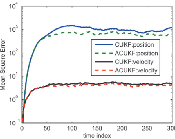
CLMS and their corresponding widely linear versions . . . 71 3.5 Performances of CUKF and ACUKF with second order noncircular state noise (K= 0.9) . 72

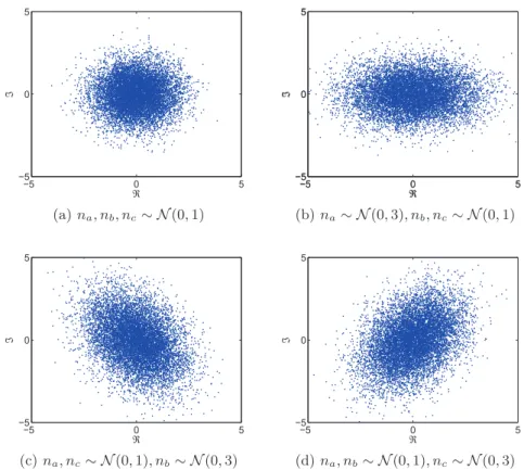
4.1 An illustration of the trajectory of Clarke voltagevkfor different operating conditions. For a balanced system, characterised byVa,k=Vb,k=Vc,k, the trajectory ofvk is circular, while, for unbalanced systems, such as in the case of a 100% single-phase voltage sag illustrated by the ellipse in the figure (+), the trajectory of the output voltage becomes noncircular. . 80 4.2 Observation noise distributions after the three phase (independent, Gaussian and real

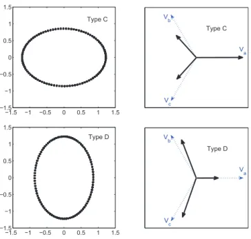
val-ued) noisesna,k,nb,k andnc,k undergo Clarke’sαβtransformation. . . 82 4.3 Geometric and phasor views of Type C and D voltage sags. The real-imaginary plots

illustrate the noncircularity of Clarke’s voltage in unbalanced conditions. The parameters of the circularity plot (ellipse) help identify the type of fault (voltage sag). . . 87

(9)

List of Figures 9

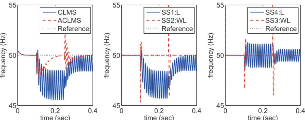
4.4 Frequency estimation for a system which is balanced up to 0.1s, after which the system becomes unbalanced due to the occurrence of voltage sags of differing natures. . . 88 4.5 Initial transient behaviour for the simulations in Figure 5 (first 5ms), where all the Kalman

filters where initialised asMa

k|k= 10I. . . 88 4.6 Frequency estimation for a balanced system in the presence of doubly white circular Gaussian

noises at 20dB SNR. . . 89 4.7 Frequency estimation when phase voltages are contaminated with in-phase harmonics at

10% p.u. for the 3rd and 5% p.u. for the 5th harmonics. . . 89 4.8 Frequency estimation for a power system which experiences a 5Hz/s rise and decay in system

frequency. . . 90 4.9 Mean square error (MSE) and bias analysis for an unbalanced system undergoing a voltage

sag (Type D). . . 91 4.10 Frequency estimation for a system which experiences a temporary step change in frequency

from 50Hz to 52Hz in the presence of white circular Gaussian noises at 35dB SNR. In (a) the frequency is estimated using SS3 and SS4 with fixed state and observation noise variances, while in (b) the state noise variance was set according to the innovation power using the methodology described in Section 4.3. . . 92 4.11 An initially balanced system experiences a series of voltages sags, all in the presence of

complex doubly white measurement noise. . . 92 4.12 Frequency estimation for a real-world three-phase system, where an initially balanced system

experienced a single-line short with earth. . . 93 4.13 Frequency estimation for a real-world unbalanced three-phase system, where two lines

ex-perience a short with earth. . . 94

5.1 An illustrative example of a distributed network topology. . . 99 5.2 A distributed network withN= 10 nodes used in the simulations. . . 111 5.3 Steady state performance comparison for filtering the AR(2) process in the cases of: (a)

circular observation noises and a noncircular driving noise with varying degrees of noncir-cularity; (b) circular state noise and noncircular observation noises with varying degrees of noncircularity, whereby all nodes have same degree of observation noise noncircularity. . . . 112 5.4 A distributed network withN= 20 nodes used in the simulations. . . 113 5.5 projectile tracking simulations: (a) Average performance (of all the nodes) for a trial run of

the diffusion algorithms; (b) Transient performance of the centralised and diffusion algorithms.114

6.1 Comparison between thel1- andl2-norm regularised cost functions for different values ofγ. The standard cost function is achieved by settingγ= 0. . . 120 6.2 Coefficient convergence of the ACLMS and R-ACLMS for a strictly linear system with a

noncircular input signal. . . 124 6.3 Performance comparison between the CLMS, the widely linear ACLMS, thel1- andl2-norm

regularised ACLMS (R-ACLMS) for strictly and widely linear systems with a circular input vectorE{x_kxT

k}=0. . . 126 6.4 Performance comparison between the CLMS, the widely linear ACLMS, thel1- andl2-norm

regularised ACLMS (R-ACLMS) for strictly and widely linear systems with a noncircular input vectorE{x_kxT

k}= 0.6I. . . 126 6.5 Performance comparison between the different algorithms for the prediction of real-world

(10)

A.1 Steady-state performance comparison between the conventional complex particle filter (CCPF) and the augmented complex particle filter (ACPF) for the AR(1) filtering problem: (a) circular observation noise and a noncircular state noise with varying degrees of noncir-cularity; (b) circular state noise and noncircular observation noise with varying degrees of noncircularity. . . 145 A.2 Performance of standard and augmented complex filters for BOT problem with noncircular

state and observation noises. . . 147

B.1 A geometric view of the three sonobouy sensors (top view). . . 151 B.2 Performance comparison between the proposed augmented complex state space approach

and the arctan estimator for the case where the target source signal is a sinusoid. . . 156 B.3 Performance comparison between the proposed augmented complex state space approach

and the arctan estimator for the case where source signal is an autoregressive process with (a) a Gaussian; (b) a uniform driving noise. . . 157

(11)

11

Statement of Originality

I declare that the content embodied in this thesis is the outcome of my research under the guidance of my thesis adviser Prof Danilo P. Mandic. Any ideas or quotations from the work of other people, published or otherwise, are fully acknowledged in accordance with the standard referencing practices of the discipline. The material on this thesis has not been submitted for any degree at any other academic or professional institution.

(12)

Publications From This Thesis

Patent

A patent application regarding frequency estimation and fault identification in three phase power systems and smat-grids - UK Patent Application No. 1217737.4 (ref: 6279), October 2012.

Journal papers

[1] D.H. Dini, D.P. Mandic, S.J. Julier, “A Widely Linear Complex Unscented Kalman Filter,” IEEE Signal Processing Letters, vol.18, no.11, pp.623-626, Nov. 2011

[2] D.H. Dini, C. Jahanchahi, D.P. Mandic, “Widely Linear Complex and Quaternion Valued Bearings Only Tracking,” IET Signal Processing Special Issue on: Multi-Sensor Signal Processing for Defence, vol.6, no.5, pp.435-445, July 2012

[3] D.H. Dini, D.P. Mandic, “Class of Widely Linear Complex Kalman Filters,” IEEE Transactions on Neural Networks and Learning Systems, vol.23, no.5, pp.775-786, May 2012

[4] D.H. Dini, D.P. Mandic, “Widely Linear Modeling for Frequency Estimation in Unbalanced Three-Phase Power Systems,” IEEE Transactions on Instrumentation and Measurement, vol.62, no.2, pp.353-363, Feb. 2013

[5] D.H. Dini, P.M. Djuric, D.P. Mandic, “The Augmented Complex Particle Fil-ter,” IEEE Transactions on Signal Processing, vol.61, no.17, pp.4341-4346, Sept. 2013

(13)

Publications 13

Conference papers

[6] D.H. Dini, D.P. Mandic, “Analysis of the Widely Linear Complex Kalman Filter,” Proceedings of Sensor Signal Processing for Defence (SSPD), Sep. 2010

[7] D.H. Dini, D.P. Mandic, “Widely Linear Complex Extended Kalman Filters,” Proceedings of Sensor Signal Processing for Defence (SSPD), Sep. 2011

[8] D.H. Dini, D.P. Mandic, “Widely Linear State Space Models for Frequency Es-timation in Unbalanced Three-Phase Systems,” Proceedings of IEEE 7th Sensor Array and Multichannel Signal Processing Workshop (SAM), 2012, pp.9-12, 17-20 June 2012

[9] D.H. Dini, D.P. Mandic, “An Enhanced Bearing Estimation Technique for DI-FAR Sonobuoy Underwater Target Tracking,” Proceedings of Sensor Signal Processing for Defence (SSPD), Sep. 2012

[10] D.H. Dini, D.P. Mandic, “Cooperative Adaptive Estimation of Distributed Noncircular Complex Signals,” Proceedings of ASILOMAR, pp.1518-1522, 4-7 Nov. 2012

[11] D.H. Dini, D.P. Mandic, “Exploiting Sparsity in Widely Linear Estimation,” Proceedings of the 10th International Symposium on Wireless Communication Systems (ISWCS), vol., pp.1-5, Aug. 2013

(14)

Chapter 1 Introduction

W

E live in an information age. The recent advances in sensor and computing technologies have not only vastly increased the availability of data, but also the capabilities to robustly deal with large data sets. Moreover, as technology continues to evolve, the need to make sense and inferences from ever more complex data takes ever greater precedence, and next generation techniques and solutions for achieving enhanced performance become paramount.

Another facet of modern technology is the reliance on multiple sensors, whereby measurements from a number of sensors, often with overlapping information, need to be simultaneously processed to enhance performance and increase system capabilities. How-ever, in distributed systems consisting of sensor spread over a certain geographical region, such centralised methodologies requires large communication overheads, and distributed estimation frameworks, which relies on cooperation between neighbouring sensors, are often preferred to reduce the computational and communication overheads.

Typically, real-world data are corrupted by noise and interferences, exhibit laten-cies and coupling, and are nonstationary; and hence do not directly yield to analysis and information extraction. This necessitates mathematical data processing techniques that simultaneously facilitate the extraction of useful information, and the suppression of redundant interferences.

(15)

in-1. Introduction 15

formation retrieval from noisy corrupted data, and forms the backbone of many modern technologies, including communications and bio-medicine. Signal processing encompasses a large array of techniques ranging from image and audio processing to data compres-sion and weather forecasting, however, as the need for more advanced data processing technologies increases, so does the requirement for the development of next-generation signal processing solutions capable of meeting the challenges of efficient, low-cost, fast and accurate data processing frameworks.

This thesis is on the subject of signal processing, and more specifically adaptive filters. Unlike other signal processing techniques, adaptive filters operate and optimise their performance in real-time with the arrival of new information, which has made them ubiquitous in many time-constrained technologies, such as satellite navigation, wireless communication, electrical smart-grids and brain-computer-interfaces. The aim of this re-search is focused on the development a novel theoretical framework and enhanced practical solutions for adaptive processing of complex valued signals, that is, signals with real and imaginary components.

Complex numbers are not artificially constructed concepts, but occur naturally when solving real valued problems. Although complex numbers came to prominence in the 16th century, they were not fully mainstream in the science community until the 19th century, when their geometrical interpretation was described and their usefulness in dealing with trigonometric identities identified.

Complex signals arise in a numerous real-world practical applications, as well as in transform domains such as Fourier and wavelet, where real valued data becomes com-plex after processing. The comcom-plex domain has distinct advantages including providing a convenient representation of bivariate data, and a natural way for preserving the charac-teristics of signals and the transformations they undergo, such as phase and magnitude distortions in communication systems.

Complex signal processing is the enabling technology behind applications, such as mobile communication and magnetic source imaging, however, standard, widely used, solutions inherently assumeproper signal distributions. This is generally inadequate, given

(16)

that real-world signals almost invariablyimproper, and treating all signals as proper leads to algorithms that are unable to fully utilised the available information.

The work presented here is based on recent developments in the statistics of complex variables, called augmented complex statistics, and is used in conjunction with widely linear adaptive signal processing, to enable optimal processing for the generality of complex signals, both proper and improper. Augmented complex statistics allows for full utilisation of the available second order statistics of complex signals. Further, the effects of improper signals on the behavior of various algorithms, where second order propriety are normally assumed, is also examined. A number of widely linear (augmented) complex algorithms are proposed and analysed here, and their behavior are illustrated in a number of application employing real-world and synthetic data.

These include the gradient descent based least mean square together with the adap-tive state space based Kalman and particle filtering techniques, which allow the modelling and estimation of nonstationary systems, and proposes solutions to enhance the perfor-mance of these techniques for improper data sources and widely linear system models.

This thesis is organised as follows. Each technical chapter and appendix starts with an introduction clearly detailing the original contribution of the author to the work contained within. Chapter 2 deals the background theory regarding complex signals, while Chapter 3 is the first technical chapter, and presents complex valued Kalman filters which are second order optimal for the generality of complex data. Chapter 4 concerns the application of the proposed Kalman filters for frequency estimation in unbalanced three phase power systems, whereas Chapter 5 extends the work in Chapter 3 to the case of distributed state space estimation in the presence of correlated measurement noises. In Chapter 6 some convergence issues of the gradient descent based augmented complex LMS (ACLMS) algorithm are addressed. Lastly, the chapter in Appendix A, explores the benefits of utilising density functions which cater for improper distributions within the framework of complex valued particle filters, while, the chapter in Appendix B proposes a new solution to the DIFAR sonobuoy bearing estimation problem for underwater acoustic sources based on the algorithms introduced in Chapter 3.

(17)

1. Introduction 17

Novel Contributions

The main contributions of this thesis are presented in the following Chapters, however, concise summaries along with the relevant publications are presented below.

1. We introduce a class of widely linear complex Kalman filters, namely the aug-mented complex Kalman filter (ACKF), augaug-mented complex extended Kalman filter (ACEKF) and augmented complex unscented Kalman filter (ACUKF), suited to the generality of complex signals, and analyse their performances under proper and im-proper signals. For rigour, a theoretical bound for the performance advantage of widely linear Kalman filters over their strictly linear conventional complex Kalman filters (CCKFs) is provided. The analysis also addresses the duality with bivariate real valued Kalman filters, together with several issues of implementation, and the Cramer-Rao lower bound (CRLB) for the widely linear Kalman filters is established. Our mean square analysis shows that the performance of CCKF is unaffected by the impropriety of the state and observation signals, however, the mean square char-acteristics of the complex extended Kalman filter (CEKF) and complex unscented Kalman filter (CUKF) are a functions of the impropriety of the state noise impro-priety [1].

2. We revisit real-time frequency estimation in three phase power systems from a state space point of view, in order to provide a unified framework for frequency tracking in both balanced and unbalanced system conditions. We achieve this by using widely linear complex valued Kalman filters which are faster converging and more robust to noise and harmonic artifacts than the existing methods . It is shown that the Clarke’s transformed three phase voltage is circular for balanced systems and noncircular for unbalanced ones, making the proposed widely linear estimation perfectly suited to both identify the fault and to provide accurate estimation in unbalanced conditions, critical issues where standard models typically fail. Our analysis and simulations show that the proposed approaches outperform the recently introduced widely linear stochastic gradient based frequency estimators, based on the augmented complex

(18)

least mean square (ACLMS) [2].

3. We introduce cooperative sequential state space estimation in the domain of aug-mented complex statistics, whereby nodes in a network collaborate locally to esti-mate improper complex signals. For rigour, a distributed augmented (widely linear) complex Kalman filter (D-ACKF) suited to the generality of complex signals is in-troduced, allowing for unified treatment of both proper (rotation invariant) and improper (rotation dependent) signal distributions. Our analysis and simulations show that unlike existing distributed Kalman filter solutions, the D-ACKF caters for both the improper data and the cross-correlations between the observation noises at neighbouring nodes, encountered when nodes are exposed to common noise (e.g. jamming noise), thus providing enhanced performance in real-world scenarios [3].

4. The distribution of complex random signals is typically improper, and conventional strictly linear models are only second order optimum for signals with proper distribu-tions, while widely linear models are optimum for both proper and improper signals. Widely-linear models, however, are over-parameterised when the underlying system is strictly-linear, requiring twice the number of parameters to be estimated compared to strictly-linear models. This effects widely linear adaptive algorithms, such as the augmented complex least mean square (ACLMS) and augmented complex recursive least squares (ACRLS), and leads to slow convergence. We here address the prob-lem of the over-parameterisation of the ACLMS through the use of regularised cost error functions. The conjugate weight regularised ACLMS (R-ACLMS) algorithm is presented and shown to converge faster than the ACLMS, while offering similar steady-state performance for strictly linear systems [4].

5. Current complex valued particle filters (PFs) have assumed (implicitly or explicitly) circular signal distributions, which for noncircular signals leads to suboptimal per-formance. We employ augmented complex statistics, and propose the augmented complex PF (ACPF) and the augmented complex Gaussian PF (ACGPF) for the sequential estimation of complex states in both circular and noncircular noise, and show through simulations the advantages for the proposed solutions [5].

(19)

1. Introduction 19

6. We address the DIFAR sonobuoy bearing estimation problem for underwater acoustic sources. The standard arctangent based approach utilises the orthogonality between the observation noises for the different channels to form the bearing estimates, and ignores the correlation structure of the actual source signal. We propose a new state space technique, which exploits the correlations structure in the source signal to achieve enhanced performance, particularly in low signal-to-noise (SNR) conditions, compared to the standard arctangent estimator [6].

(20)

Chapter 2 Background

This chapter presents a background on complex numbers and a few topics on complex valued signal processing. This chapter contains a summary of the introductory chapters in [7], together with some works from [8] [9] [10] [11]. For more a complete overview of this subject, see the above references and the other works cited within this Chapter.

2.1 History of Complex Numbers

The concept of a “new number” has often arose because of a need to solve a practical problem. For instance to solve for the diagonal of a unit length square (√12_{+ 1}2 ₌√_2),

irrational numbers needed to be introduced, whereas calculating the circumference of a circle required the use of the irrational π. Likewise complex numbers came from the necessity to solve equations involving the square root of negative numbers such asx2 ₌₋_4.

Complex numbers arose to prominence in the 16th century when the Italian math-ematicians Niccolo Fontana Tartaglia and Gerolamo Cardano sought to find closed form solutions to the roots of cubic and quartic polynomials. This led to expressions involving the square roots of negative numbers. They realized that even when only searching for real solutions, the manipulation of square roots of negative numbers was often required. For instance, Tartaglia’s cubic formula

(21)

2.1 History of Complex Numbers 21

has the following solution

1

√

3

(√₋1)13 + 1

(√₋1)13

(2.2)

and when the three cube roots of ₋1 are substituted into this expression the three real roots, 0, 1 and₋1 are found. Rafael Bombelli was the first to explicitly address these seem-ingly paradoxical solutions of cubic equations and developed the rules for manipulating complex numbers. In solving for the roots of

x3₋15x₋4 = 0 (2.3)

he was able to show that

2 +√₋1+2₋√₋1= 4 (2.4)

whereby, it was necessary to perform calculations in the field of complex numbers C _in

order to compute the real roots.

Complex numbers gained notoriety in the 18th century, as it was noted that com-putations involving trigonometric expressions could be simplified by utilising complex expressions. Abraham de Moivre, for example, used formal manipulation of complex ex-pressions to show that identities relating trigonometric functions of an integer multiple of an angle could be re-expressed as powers of trigonometric functions of that same angle using the formula which bears his name, that is

(cosθ+jsinθ)n= cosnθ+jsinnθ. (2.5)

In 1748 Leonhard Euler went further and proposed the well-known Euler formula:

cosθ+jsinθ=ejθ (2.6)

which reduces trigonometric identities to their simple exponential equivalents.

(22)

geometrical interpretation was described by Caspar Wessel in 1799. Carl Friedrich Gauss rediscovered these interpretations several years later and popularised it, and as a conse-quence the theory of complex numbers received a notable expansion. Although, the ideas behind the geometric representation of complex numbers had appeared as early as 1685, in Wallis’s De Algebra Tractatus.

2.2 Motivations for Complex Valued Signal Processing

Complex valued signals and algorithms have proven to be useful in a wide range of theoret-ical and practtheoret-ical applications. The complex domain is the natural home for the represen-tation and processing of numerous commonly encountered data, however, the usefulness of complex valued signals is generally application dependent. Next some applications, motivations and benefits behind complex valued systems and signals are discussed.

2.2.1 Examples of Complex Valued Signals

Fourier Analysis. The Fourier series decomposes periodic functions or signals into the sum of simple oscillating functions, namely complex exponentials. Fourier series were introduced by Joseph Fourier (1768−1830) for the purpose of solving the heat equation in a metal plate. The real valued function f[x] with a finite number of discontinuities and extrema has a Fourier series representation given by

f[t] =

+∞ X

n=−∞

cnejωnt (2.7)

where the Fourier coefficients _{cn} are computed as

cn=

1 T

Z t2

t1

f[t]e−jωnt_dt _(2.8)

and T =t2−t1 is the period of the function f[t].

The Fourier series along with the Fourier transform are perhaps the most widely used form of complex representation of real valued data. The original concept of Fourier

(23)

2.2 Motivations for Complex Valued Signal Processing 23

analysis has been extended over time to apply to more abstract and general situations, and the general field is often known as harmonic analysis. The applications of Fourier analysis are many and vary from filter bank design to modern cell phones or radio scanners.

Phasors. In mathematics and signal processing, a phase-vector (“phasor”) is a very useful technique for conceptualising sinusoidally oscillating quantities. A phasor can be seen as a rotating vector. For instance, Euler’s formula indicates that a sinusoidal signal x[t] =|x|cos[ωt+φ] can be represented as

x[t] =_ℜ{|x_|ejφ_·ejωt_} (2.9)

where the operatorℜ{·}denotes the real part of a complex number. The phasor can refer to either_|x_|ejφ_·_ejωt_{or just the complex constant}_|_x_|_ejφ_{. In the latter case, it is understood}

to be a shorthand notation, denoting the amplitude and phase of the underlying sinusoid function.

Phasors are used for the analysis of systems involving oscillating signals, such as three phase alternating current (AC) power systems, where three phasors, of equal mag-nitude and phases at 0, 120 and 240 degrees, are used to represent the three oscillating voltages. Phasor representations of the polyphase AC circuit variables allows for balanced systems to be simplified and unbalanced systems to be dealt with as algebraic combi-nations of symmetrical systems. This approach greatly simplifies the work required in calculating voltage drops, power flows, and short-circuit currents.

Analytic signals. Signals with no negative-frequency components are known as ana-lytic. The analytic representation of a real valued function or signal facilitates mathe-matical manipulations, and offers a convenient way to obtain phase and instantaneous frequency information. The idea behind analytic signals is to remove the redundant fre-quency spectrum, that is due to the symmetry of the Fourier transform (spectrum) of real-valued function, the negative frequency components can be discarded without loss of information.

(24)

defined as

Xa[f] =

              

2X[f], iff >0

X[f], iff = 0 0, iff <0

= X[f]_·2u[f] (2.10)

only contains the non-negative frequency components ofX[f], whereu[f] is the Heaviside step function. The inverse function exists due to symmetry of the spectrum of X[f], that is

X[f] =                1

2Xa[f], iff >0

Xa[f], iff = 0

1

2Xa∗[|f|], iff <0

(2.11)

where (_·)∗ is the complex conjugate operator. The complex valued time domain represen-tation of Xa[f] is the analytic version ofx[t], and is given by

xa[t] = F−1{Xa[f]}

= F−1{X[f]} ∗ F−1{2u[f]}

= x[t] +j!x[t]∗ 1 πt

(2.12)

where the symbol _∗denotes the convolution operator andx[t]_∗_πt1 is the Hilbert transform of x[t].

Analytic representations of real signals are commonly utilised in signal process-ing and communication systems, whereby complex envelopes facilitates modulation and demodulation techniques together with the analysis of signals properties.

Native complex signals. Some signals can be seen as naturally complex, where an in-phase and a quadrature component is the natural representation which enables the full relationship between two components to be taken into account. Examples include radar

(25)

2.2 Motivations for Complex Valued Signal Processing 25

and directional processes as well as many communication signals such as binary phase shift keying (BPSK), quadrature phase shift keying (QPSK) and quadrature amplitude mod-ulation (QAM). The MRI (magnetic resonance imaging) signal is also naturally complex because two orthogonal detectors are used to capture the images.

The complex domain can also be used to capture the magnitude and phase rela-tionship between two real-valued signals. For example, wind signals have magnitude (wind intensity) and phase (wind direction), and have a natural complex representation.

2.2.2 Other Benefits of Complex Valued Processing

In addition to the examples above, signal processing in the complex domain has several distinct features and advantages; some of which are discussed below.

More powerful statistics. Recent developments in complex statistics have shown that statistics in C _{are not simple extensions of statistics in} R_{. The notions of proper and}

improper complex random variables, gives more degrees of freedom and hence greater potential for improved performance compared with standard modelling inC_{. For example}

in blind source separation and extraction problems, complex signals with varying degrees of impropriety can be separated.

Simultaneous modelling and fusion of two variables. Complex domain modelling of directional processes, such as wind, not only provides a convenient representation, but also provides sequential data fusion. The magnitude and phase, which are of different natures, are fused to into a single scalar quantity.

Visualisation. Whereas real valued functions are represented by two dimensional graphs, complex functions are represented by four dimensional graphs (two axis for the real and imaginary parts of the function argument and two axis for the real and imaginary parts of the evaluated function). Hence to visualise a complex function, the two dimensional func-tion argument is plotted against either the phase or magnitude of the evaluated funcfunc-tion or the graph is colour coded to suggest the fourth dimension.

(26)

Compact and natural representation. The complex numberx=a+jbcan be thought of as a single entity that satisfies all the standard rules of algebra. For algorithms such as the least mean square (LMS) or recursive least squares (RLS), where the desired signal (training signal) is a scalar, a complex version of these algorithms allows the desired signal to become bivariate because a scalar complex signal consists of real and imaginary parts. To account for a bivariate desired signal in real valued LMS and RLS algorithms, two filters need to be implemented.

An alternative domain. The complex domain offers an alternative to the real domain for formulating solutions. This is useful in numerous application, such as deriving recursive expressions to problems, which are necessary in adaptive filters. For example, consider the recursive expression for an exponential:

ejωk=ejωejω(k−1)

where k is the time index. The recursive nature of the real valued equivalent to this expression is not as intuitive, that is

ejωk= (cos[ω] +jsin[ω])(cos[ω(k₋1)] +jsin[ω(k₋1)])

= cos[ω] cos[ω(k−1)]−sin[ω] sin[ω(k−1)] +jcos[ω] sin[ω(k−1)] +jsin[ω] cos[ω(k−1)]

Similarly, the recursive forms for sinusoids, for example cos[ωk] = 1/2ejωk+ 1/2e−jωk, are more elegantly expressed as complex exponentials. Further, the complex domain can be considered a generalisation of the real domain, in that when the imaginary part vanishes, the two domains are equal.

Homomorphic filtering. Typically noise is additive, that is the observation consists of the summation of a signal and noise. However, there are often cases involving multiplica-tive noise, where the observation consists the product of a signal and noise. One approach for dealing with multiplicative signals is through homomorphic filtering, whereby the log-arithm of the product is used to separate the signals, for example lnxy = lnx+ lny. For real valued variables, the logarithm does not exist for x≤0 ory≤0, while the logarithm

(27)

2.3 Complex Statistics and Widely Linear Estimation 27

of a nonzero complex signal z=_|z_|ejθ _{is always defined as ln}_z_{= ln}_|_z_|₊_jθ_.

Derivative approximation. The first order Taylor series approximation of a real valued functionf[_·] with a real argument ais defined as

f′[a] = f[a+h]−f[a]

h +O[h]

where h is the real valued argument increment. On the other hand, the Taylor series approximation for a complex valued argument is given by

f[a+jh] =f[a] +jhf′[a]₋ 1 2!h

2_f′′_[_a_]₋ 1 3!jh

3_f′′′_[_a_{] +}_{· · ·}

where f′′[_·] and f′′′[_·] are the second and third order derivatives. Equating the imaginary parts yields

f′[a] = ℑ{f[a+jh]} h +O[h

2_]

The operator ℑ{·}is the imaginary part of a complex number. Observe that there is no difference operation and the error is anO[h2] operation when the argument is complex val-ued, hence the derivative is be better approximated by utilising a complex representation, given that h <<1 is typically chosen.

The importance of phase information. In a number of real world applications, the phase information is more important the magnitude information, e.g. image processing. Consider Figure 2.1 showing two original images along with the cases where their phase spectra are interchanged prior to taking the inverse Fourier transform. It is clear that most of the meaningful information is contained in the phase, as the appearance of the phase exchanged images are dominated by the phase information.

2.3 Complex Statistics and Widely Linear Estimation

The distribution of signals dictate the signal processing techniques and the nature of the estimators suited to dealing with them. For example, the optimal estimator, in the mean

(28)

(a) Image I1: Buffalos (b) Image I2: Elephants

(c) I3 =F−1n_F₍_I₁₎_exp(_j

∠F(I2))o (d) I4 =F−1n_F₍_I₂₎_exp(_j

∠F(I1))o

Figure 2.1: An illustration of the importance of phase in pictures. The Figures (a) and (b) are the original images, while figure (c) consists of the magnitude information from (a) and the phase information from (b), and vice versa for Figure (d). The visual perceptions of (c) and (d) are largely dominated by the phase information.

square error sense, for a linear Gaussian process is linear, while for nonlinear or non Gaussian processes the optimal estimator is generally untenable. Hence a thorough un-derstanding of the distribution of complex signals, plays a fundamental role in developing the right algorithms for different problem sets. In this section, the statistical moments of complex signals are discussed with special emphasis on the second order moments.

(29)

2.3.1 Second Order Statistics of Complex Signals

Second order statistics plays an important role in signal processing. Typically, the esti-mation error does not directly yield to minimisation due to non-convexity, and we seek to minimise convex functions of the estimation error. Among the possible choices, it is the mean square error (MSE) and its approximates which are often the default choice, given that for an unbiased estimator the MSE is equal to the error variance (power), while for biased estimator it is equal to sum of the error variance and the squared bias - thus MSE is essentially a second order statistical moment. From a practical view point, lower MSE corresponds to better estimation performance.

The prominence of complex signals necessitates the need for a deeper understanding of their statistics. The second order statistical properties of a zero mean1 complex vector z=x+jyhas conventionally been characterised by its covariance matrix Rz =E{zzH}, where (_·)H _{indicates the complex-conjugate transpose operator. However, this is}

insuf-ficient for a complete second-order description, and another moment function known as the pseudocovariance (also referred to as the relation function or complementary covari-ance) Pz = E{zzT}, where (·)T is the transpose operator, is also necessary. It is only for the special class of complex signals known as second order proper orcircular, that is, those with rotation invariant probability distributions, characterised by a vanishing pseu-docovariance, that their covariance function suffices to give the complete second order description. The covariance matrix captures the information regarding the total power of the signal, while the pseudocovariance captures the information about the power difference and cross-correlation between the real and imaginary parts of the signal.

The term circularity comes from the following remarks. It is clear that the covari-ance of z and its rotated version¯z=zejθ are equal for any real number θ. However, the pseudocovariances of z and¯z are equal if and only if

Pz=E{zzT}=P¯z =E{¯z¯zT}=ej2θE{zzT}=ej2θPz (2.13)

(30)

−3 −2 −1 0 1 2 3 −3

−2 −1 0 1 2 3

ℜ

ℑ

(a) Circular distribution

−3 −2 −1 0 1 2 3

ℜ

ℑ

(b) Uncorrelated noncircular

−3 −2 −1 0 1 2 3

ℜ

ℑ

(c) Correlated noncircular

−3 −2 −1 0 1 2 3

ℜ

ℑ

(d) Correlated noncircular

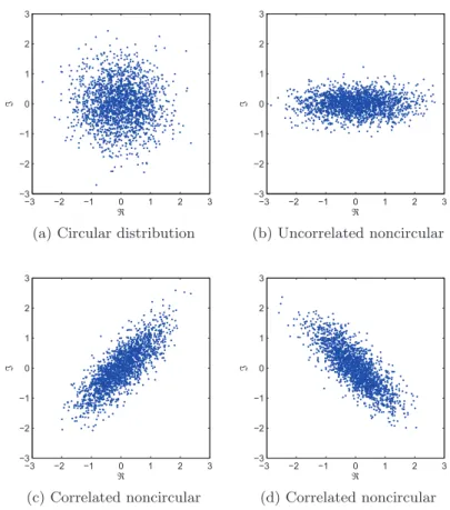
Figure 2.2: A geometric view of circularity via a real-imaginary scatter plot of zero-mean complex white Gaussian distributions.

which leads to the solution Pz = 0. A circular signal is a signal whose second order statistics are invariant for any phase rotation, thus the pseudocovariance vanishes for circular signals.

At this point it is worth noting that signals with zero pseudocovariances do not necessarily have circular distributions, however, signals with circular distributions always have zero pseudocovariances as shown in (2.13). Gaussian signals are a special case for whom a vanishing pseudocovariance implies circularity and vise-versa is also true.

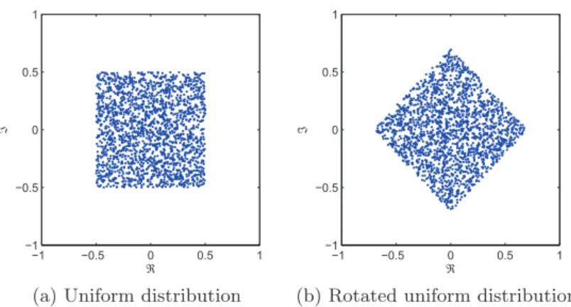
To illustrate this point consider Figure 2.2 which shows a geometric view of the circularity of complex Gaussian distributions with identical variances with varying pseu-docovariances. Figure 2.2a shows a circular signal with zero pseudocovariance, while the remaining figures have the same pseudocovariance magnitude. On the other hand, Fig-ure 2.3 show a uniform distribution and its 45 degree rotated version, both have zero

(31)

−1 −0.5 0 0.5 1

ℜ

ℑ

(a) Uniform distribution

−1 −0.5 0 0.5 1

ℜ

ℑ

(b) Rotated uniform distribution

Figure 2.3: A real-imaginary scatter plot of zero-mean complex white uniform distri-butions with zero pseudocovariances (both are proper).

pseudocovariances, but are noncircular.

To differentiate between these scenarios, for the remainder of this thesis, we will use the term proper to refer to all signals with vanishing pseudocovariances, and the term circular to refer to signals with rotation invariant distributions, which also implies zero pseudocovariances. Hence, the term proper is more general, and circular is as a special case of proper. Further, for real valued signals the covariance and pseudocovariance are equal, and as such real signals are always improper (noncircular).

The covariance matrixRz by its definition is positive semi-definite, while the pseu-docovariance matrix Pz is symmetric. To illuminate this, consider the decomposition of these two matrices in terms of the covariances and cross-correlations between the real and imaginary parts of the complex vector z=x+jy, namely

Rz = E{zzH}

= Rx+Ry+j(Ryx−Rxy) (2.14)

Pz = E{zzT}

= Rx−Ry+j(Rxy+Ryx) (2.15)

where Rx=E{xxT},Ry =E{yyT}and Rxy =RyxT =E{xyT}. Based on (2.15), ob-serve that for a complex signal to be circular, that is Pz=0, implies two strict conditions

(32)

on the real (x) and imaginary (y) parts of the signal, namely

1. x andy have identical covariances: Rx=Ry

2. x andy are orthogonal: Rxy =0

If either of these conditions is not met, the complex signal is then improper.

2.3.2 Complex White Noise

The concept of white noise is critical in signal processing, as it allows for modelling of uncertainties in systems. However, the framework for defining complex white noise is not a straight forward extension of real white noise. A wide sense stationary signalz[k] is white if its covariance function cz[τ] =E{z[k]z∗[k−τ]}is a Dirac delta function or equivalently

its power spectrum Γz[f] =F{cz[τ]} (the Fourier transform of cz) is constant, that is

cz[τ] =aδ[τ] ⇔ Γz[f] =a= constant (2.16)

The definition of whiteness also enforces constraints on the pseudocovariance function pz[τ] = E{z[k]z[k −τ]} or the spectral pseudocovariance Pz[f] = F{pz[τ]} (the Fourier

transform of pz), through the relationship between the covariance and pseudocovariance

functions, see (2.14) and (2.15). It can be shown that given the power spectrum, the spectral pseudocovariance satisfy the following conditions [8]:

Γz[f] ≥ 0

Pz[f] = Pz[−f]

|Pz[f]|2 ≤ Γz[f]Γz[−f] (2.17)

Hence, if a signal is second order stationary and white we have

cz[k] = cδ[k]

(33)

which implies that the absolute square of the spectral pseudocovariance is a constant with a value between zero and a2_{. The spectral pseudocovariance function} _P

z[f] is often

assumed to be zero, which means that the white signal is proper. However, for a non-zero pseudocovariance function Pz[f], we can have improper white noise. Therefore we can

define two types of stationary complex white noises:

1. Proper white noise characterised by a constant power spectrum and a vanishing pseudocovariance function. The real and imaginary parts of the signal have equal variance and are uncorrelated, that is

cz[τ] =aδ[τ] and pz[τ] = 0 (2.19)

While the frequency domain equivalent is given by

Γz[f] = a= constant

Pz[f] = 0 (2.20)

2. Doubly white noise characterised by

cz[τ] =aδ[τ] and pz[τ] =bδ[τ]

where the only condition on the pseudocovariance function is |b| ≤ a. The power spectrum and the spectral pseudocovariance are then given by

Γz[f] = a= constant

Pz[f] = b= constant (2.21)

2.3.3 Widely Linear (Augmented) Complex Estimation

To introduce an optimal second order estimator for the generality of complex signals, consider the minimum mean square error (MSE) estimator of a real valued random vector y in terms of an observed real vector x, that is, ˆy = E_{y_|x_}. For zero-mean, jointly

(34)

normal y andx, the optimal estimator is linear, that is

ˆ

y=Ax (2.22)

The aim is then to find the coefficient matrix Athat minimises the MSE given by

Σl =E{[y−Ax][y−Ax]H} (2.23)

Differentiating Σl _{with respect to}_A_{, and setting the derivative to zero yields the solution}

A=RyxR−x1 (2.24)

whereRyx=E{yxH}. Standard, ‘strictly linear’ estimation inCassumes the same model but with complex valued y =yr+jyi and x=xr+jxi, and the resulting solution has

the same form: A=RyxR−x1 but is complex valued. Observe that this solution does not incorporate the pseudocovariance of the data, and is hence blind to the propriety of the signals.

Next consider the bi-variate estimation problem, whereby the aim is to estimate each of yr and yi based onxr andxi, that is

ˆ

yr=E{yr|xr,xi} (2.25)

ˆ

yi =E{yi|xr,xi} (2.26)

Substituting in the complex representations for xr = (x+x∗)/2 and xi = (x−x∗)/2

yields

ˆ

yr =E{yr|x,x∗} (2.27)

ˆ

yi=E{yi|x,x∗} (2.28)

which highlights that y needs to be estimated in terms of both x and its conjugate x∗. The optimal complex estimator can be derived formally by considering the problem of

(35)

estimatingy asE_{y_|x,x∗_}_{. The MSE is then given by}

Σwl =E_{[y₋Bx₋Cx∗][y₋Bx₋Cx∗]H_} (2.29)

Next differentiating Σwl _{with respect to} _B _and _C_{, and setting the derivatives to zero}

results in the widely linearcomplex estimator2_{, that is}

ˆ

y=Bx+Cx∗ (2.30)

where the coefficient matrices are given as

B=RyxD+PyxE∗ C=RyxE+PyxD∗

with D= (Rx−PxRx∗−1P∗x)−1 andE=−(Rx−PxR∗−x 1Px∗)−1PxR∗−x 1.

The widely linear estimator (2.30) is optimal for the generality of complex signals, both proper and improper, as it caters for the covariance and pseudocovariance of the data. Observe that when y and x are jointly proper Pyx = E{yxT} = 0, and x is properPx=0, the widely linear linear solution degenerates to the standard strictly linear solution (2.22), that is C=0.

For convenience of representation, the widely linear model can be cast into an augmented representation3_:

ˆ

y=Bx+Cx∗ =Wxa (2.31)

where xa_{= [}_xT_,_xH_]T _{is the augmented input vector, and} _W_{= [}_B_,_C_{] the optimal}

coeffi-cient matrix. Further, the full second order information of the inputxis contained in the

2_{The term ”‘widely linear”’ indicates that the new estimator is a linear function of both}_x_and_x∗_{, while}

the standard strictly linear estimator is a linear function of onlyx.

3_{The term ‘widely linear’ model is associated with the signal generating system, whereas the} term“augmented statistics” describe statistical properties of measured signals. Both the terms are used to name the resulting algorithms.

(36)

augmented covariance matrix

Ra_x=E_{xaxaH_}=  

Rx Px

P∗_x R∗_x  

 (2.32)

and as such, estimation based on Ra_x incorporates both the covariance and pseudocovari-ance information. The augmented estimator then takes the form

A=Ryxa[Ra_x]−1 (2.33)

where Ryxa =E{yxa} is the cross correlation betweeny and the augmented input xa.

2.3.4 Benefit of Widely Linear Complex Estimation

The MSE performance difference between widely linear modelling over strictly linear mod-elling can be expressed as

∆=Σwl−Σl (2.34)

After some tedious algebraic manipulations and following the approach in [9], the MSE difference between the two estimators becomes [1]

∆= (Pyx−RyxR−x1Px)(R∗x−P∗xRx−1Px)−1(Pyx−RyxR−x1Px)H (2.35) The matrix ∆ is positive semi-definite owing to the positive definiteness of the matrix (R∗_x−P∗_xR_x−1Px). The two estimators have the same MSE for ∆ = 0, which is only the case when (Pyx−RyxRx−1Px) =0, in other words, when yand x are jointly proper Pyx = E{yxT} =0, and input x is proper Px = 0. Hence, the widely linear estimator always performs the same or better than the strictly linear estimator, in a MSE sense.

(37)

2.4 Degree of Complex Impropriety 37

2.4 Degree of Complex Impropriety

Complex random variables are classified as second order proper or improper. However, improper signals can take a wide range or degrees of impropriety. For example, when viewed geometrically, the circularity (propriety) of Gaussian signals can vary extensively, that is from a circular distribution to the extremely noncircular case where all the data are distributed on a line, for example when the real and imaginary parts are fully correlated the distribution is on a line. There is hence a need to quantify and measure the degrees of impropriety of complex variables. Further, the widely linear model has a larger com-putational overhead than the strictly linear model, and in some applications the degree of impropriety can determine whether the performance benefits of the widely linear model can offsets the extra computational overhead.

The circularity (or propriety) of a complex signal is preserved by linear transforma-tions, which include scaling and rotation, but not by widely linear transformations. For instance, if the complex vector z = [z1, ..., zn]T is proper then the linear transformation

G·z, where G is a nonsingular matrix, is also proper, while if z is improper, then its linear transform is also improper. However, under widely linear transformations, such as G_·z+H_·z∗ where both Gand Hare nonsingular, propriety is no longer preserved.

Hence, any measure of impropriety is also required to be invariant under linear transformations, but not widely linear transformations. This means that the measure must be a function of a complete set of invariants for the covariance Rz and pseudocovariance Pz under linear transformation. This has been shown to be given by the set ofcanonical correlations between z and its conjugate z∗. The canonical correlations are also known as the circularity coefficients and play a key role in independent component analysis of complex signals [11].

The first step to computing the canonical correlations, involves whitening the signal by taking the square root decomposition of the covariance matrix, that is

(38)

where the invertible matrix Rz1/2 is defined as the square root of the covariance matrix Rz. Then the vector ¯z=Rz−1/2z= [¯z1, ...,z¯n]T has covariance matrix

R¯z =E{z¯¯zH}=Rz−1/2RzRz−T /2=I (2.37) and is therefore a unit variance white random vector. The canonical correlations are de-termined from the pseudocovariance of the whitened signal ¯z, also known as the coherence matrix, that is

P¯z =E{¯z¯zT}=Rz−1/2PzRz−T /2 =M (2.38) The coherence matrix M, being a pseudocovariance matrix, is complex symmetric, M= MT, and can be decomposed usingTakagi factorisation to yield

M = FKFT

where F is a unitary matrix, that is FH = F−1, and the diagonal matrix K = diag(k1, k2, . . . , kn) contains the canonical correlations 1 ≥ k1 ≥ k2 ≥ · · · ≥ kn ≥ 0

on its diagonal.

Further, the linear transformation ´z = FH_¯_z ₌ _FH_R

x−1/2z = [´z1, ...,z´n]T, which

simultaneously diagonalises both the covariance and pseudocovariance, is said to be given in canonical coordinates. The canonical coordinates have the special property of being white with unit variance, together with a diagonal pseudocovariance matrix of canonical correlations, that is

R´z =E{z´´zH}=I (2.39)

P´z =E{z´´zT}=K (2.40)

Vectors, such as ´z, with unit diagonal covariances, that are generally improper, are often referred to as strongly uncorrelated. The strongly uncorrelating transform is a useful framework for the analysis of complex signal processing algorithms.

(39)

There are a number of plausible functions for measuring impropriety based on the canonical correlations, however, one measure stands out because it relates the entropy of a noncircular Gaussian random variable with its circular counterpart. The entropy of an improper Gaussian random vector with augmented covariance matrix Rza and the

corresponding proper Gaussian random vector with covariance matrixRzcan be expressed as [12]

Himproper =

1

2ln[(πe)

2n_det_R

za]

= ln[(πe)ndetRz]

| {z }

Hproper

+1 2ln

n

Y

i=1

(1−k_i2) (2.41)

where det is the matrix determinant operator. This illustrates the classical result that proper Gaussian random vectors maximise entropy Himproper ≤ Hproper, while the

en-tropy difference between the proper and improper signals is a function of the canonical correlations.

The circularity measure defined as [13]

d= 1− n

Y

i=1

(1−k_i2) = 1−detRza[detRz]−2 (2.42)

lends itself as the natural choice for measuring the degree of impropriety of complex random vectors. Moreover, this function is a compelling measure for several reasons:

• d is bounded as 0_≤d_≤1, whereby for d= 0 the signal is circular and ford= 1 the signal is maximally improper.

• It connects the entropy of the proper and improper cases.

• It is a measure of the linear dependence between zand z∗ and as such, can be used to design a generalized likelihood ratio test for impropriety.

• Tight bounds on the measure d can be obtained without the need to explicitly compute the canonical correlations, which can save on computational processing.

(40)

−3 −2 −1 0 1 2 3 −3 −2 −1 0 1 2 3 ℜ ℑ

(a) Circular: η= 0

−3 −2 −1 0 1 2 3

−3 −2 −1 0 1 2 3 ℜ ℑ

(b) Noncircular: η= 0.5

−3 −2 −1 0 1 2 3

−3 −2 −1 0 1 2 3 ℜ ℑ

(c) Noncircular: η= 0.9

−3 −2 −1 0 1 2 3

−3 −2 −1 0 1 2 3 ℜ ℑ

(d) Noncircular: η= 0.99

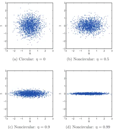
Figure 2.4: A geometric view of circularity via a real-imaginary scatter plot of white

complex Gaussian processes at different degrees of noncircularity (η), with orthogonal

real and imaginary parts.

pz=E{z2}, the measure d simplifies to:

d= |pz|

2

r2

z

(2.43)

which is essentially the square of the ratio between the pseudocovariance and covariance. This in turn motivates the ratio between the pseudocovariance and covariance, known as the circularity quotient, to be taken as an impropriety measure, that is [10]

̺= pz rz

=ηejθ (2.44)

Where η = |̺z| = √

d, 0 ≤ η ≤ 1, is the circularity coefficient4 and θ = arg(̺z) is the

circularity angle. The advantage of using the circularity quotient, over the circularity

(41)

measure d, is that it preserves the phase information contained within the pseudocovari-ance, and is simpler to compute. Figure 2.4 illustrates the distributions of white complex Gaussian noise with different degrees of noncircularity. In the following chapters, the cir-cularity coefficient will be used to test the performance of algorithms at different degrees of impropriety.

(42)

Chapter 3 Complex Valued Kalman Filters

In this first technical Chapter, we propose second order optimal complex valued Kalman filters. The Kalman filter is an adaptive state space estimation technique with a wide range of applications, including space navigation and military technology development. Complex valued Kalman filters are commonly encountered in real world scenarios such as frequency estimation [14], training of neural networks [15][7], and wireless localization [16], however, conventionally they have explicitly or implicitly been designed for assumed proper (circular) signals, that is, signals that are uncorrelated with their complex conjugates, though, real world signals are typically improper. In an earlier work [15], the widely linear complex Kalman filter was proposed in the context of neural network training, but its performance characteristics and operation in general augmented state space models were not elaborated.

In this Chapter, we propose a class of widely linear complex Kalman filters and illuminate their performances under general improper state and observation signals. The effect of signal impropriety on the mean square behavior of the conventional complex Kalman filter (CCKF), complex extended Kalman filter (CEKF) and complex unscented Kalman filter (CUKF) are analysed, and the Cramer-Rao lower bound (CRLB) for the widely linear Kalman filters is established. While, computational complexity issues are addressed by exploiting the isomorphism between the bivariate-real and complex domains. Simulations on both benchmark and real world noncircular data support the analysis.

(43)

3.1 The Augmented Complex Kalman Filter (ACKF) 43

3.1 The Augmented Complex Kalman Filter (ACKF)

Consider the standard linear state space [17]

xn = Fn−1xn−1+wn (3.1a)

yn = Hnxn+vn (3.1b)

where xn ∈ CL and yn ∈ CK are the state to be estimated and the noisy observation

(measurement) vectors at time instant n, respectively, while Fn and Hn are the state

transition and observation matrices, whereas wn ∈ CL and vn ∈ CK denote the

uncor-related state and measurement noises, respectively, and are assumed to be doubly white1

and zero-mean, hence, their covariance matrices are defined as

E  

wn

vn     

wk

vk    H =  

Qn 0

0 Rn

 

δnk (3.2)

where δnk is the Kronecker delta function, and their pseudocovariance matrices as

E  

wn

vn     

wk

vk    T =  

Pn 0

0 Un

 

δnk (3.3)

To cater for widely linear system models with improper state and observation noises, it is necessary to introduce a widely linear state space model. Based the widely linear model in (2.30), the widely linear version of the standard state space model in (3.1) is defined as2

xn = Fn−1xn−1+An−1x∗n−1+wn (3.4a)

yn = Hnxn+Bnx∗n+vn (3.4b)

1_{The term “doubly-white” refers to complex signals for which the covariance and pseudocovariance} functions are Dirac delta functions.

2_{Observe that the noise models can also be widely linear, in which case:}

w_n₌C_nw´_n₊D_nw´_n∗ _and v_n₌E_nv´_n₊G_nv´∗_{n, where}C_,D_,E_,G_{are coefficient matrices and ´}w_n_and ´

(44)

and can be expressed in a compact form using “augmented” complex vectors, such that

xa_n = Fa_n₋₁xa_n₋₁+wa_n (3.5a)

ya_n = Ha_nxa_n+v_na (3.5b)

where xa_n= [xT_n,xH_n]T and ya_n= [yT_n,yH_n]T, while,

Fa_n=  

Fn An

A∗_n F∗_n  

 and Ha_n=

 

Hn Bn

B∗_n H∗_n   

The matricesAnand Bnin (3.4) determine whether the state and observation equations

are strictly or widely linear, whereby for A = 0 and B = 0, the state space equations assume strictly linear forms. However, even for strictly linear system models, the aug-mented state space representation offers the advantage of catering for improper state and observation noises, hence providing a complete second order statistical characterisation, unlike the standard strictly linear state space model. This point was not considered in ear-lier widely linear Kalman filters. The augmented covariance matrices of the noise vectors wa_n= [xT_n,w_nH]T andv_na= [vT_n,v_nH]T, defined as

Qa_n = E_{wa_nwaH_n _}=  

Qn Pn

P∗_n Q∗_n  

 (3.6)

Ra_n = E_{v_navaH_n _}=  

Rn Un

U∗_n R∗_n  

 (3.7)

fully incorporate the noise covariance and pseudocovariance information. Once the aug-mented state space model and vectors are defined, the expressions for the augaug-mented complex Kalman filter (ACKF) can be derived in same manner as the conventional com-plex Kalman filter (CCKF) [18] but employing the augmented vectors and augmented covariance matrices. Similar to the real valued Kalman filter, the ACKF is a minimum mean square error (MSE) estimator x_ba_n_|_n=E[xa_n_|y₀a,y₁a, ...,ya_n] of xa_n based on the obser-vations {ya₀,ya₁, ...,ya_n}, when the state and observation noises are Gaussian. The ACKF is summarised in Algorithm 1.

(45)

3.1 The Augmented Complex Kalman Filter (ACKF) 45

Algorithm 1: The augmented complex Kalman filter (ACKF) Initialise with:

b

xa₀_|₀ = E_{xa₀_}

Ma₀_|₀ = E_{(xa₀₋E_{xa₀_})(xa₀₋E_{xa₀_})H_} State Prediction:

b

xa_n_|_n₋₁ =Fa_n₋₁x_ba_n₋₁_|_n₋₁ (3.8) Prediction MSE:

Ma_n_|_n₋₁=Fa_n₋₁Ma_n₋₁_|_n₋₁FaH_n₋₁+Qa_n (3.9) Kalman Gain:

Ga_n=Ma_n_|_n₋₁HaH_n !Ha_nMa_n_|_n₋₁H_naH +Ra_n−1 (3.10) State Update:

b

xa_n_|_n=x_b_na_|_n₋₁+Ga_n!ya_n−Ha_nx_ba_n_|_n₋₁ (3.11) MSE Matrix Update:

Ma_n_|_n= (I₋Ga_nHa_n)Ma_n_|_n₋₁ (3.12)

3.1.1 CCKF and ACKF Duality Analysis

For strictly linear state space models with proper state and observation noises, the CCKF and ACKF become equivalent and yield the identical state estimate at every time instant. These conditions can be summarised as follows:

Qa_n=  

Qn 0

0 Q∗_n  

,Ra_n=

 

Rn 0

0 R∗_n  

,Fa_n=

 

Fn 0

0 F∗_n  

 and Ha_n=

 

Hn 0

0 H∗_n   (3.13)

The duality between CCKF and ACKF for proper data and under the same initialisation can be illustrated as follows. Consider the prediction MSE matrix in the ACKF, which