1
EVALUATING HYDRAULIC AND
VEGETATIVE EFFECTS ON RIVER
BANK EROSION
Dario Terzic
Advisor: Dr. Karen Prestegaard
GEOL 394
2
Abstract
River bank erosion and river migration are related processes. In meandering rivers, bank erosion often drives channel migration and floodplain formation. Bank erosion rates vary among rivers, but river size (e.g. width), power (related to velocity and discharge), shape (width/depth ratio and meander shape), and bank material strength (including plant roots) all affect bank erosion rates. The goal of this research was to monitor bank erosion rates on various time scales, and to measure the hydraulic and bank material parameters that influence bank erosion rates. This was completed by: a) selecting a site near a USGS gauge for which hydraulic data are available, b) obtaining hydraulic and geomorphic data from the USGS gauge data, c) measuring exposed tree roots to monitor long-term bank erosion rates, and d) installing monitoring equipment to determine short term bank erosion rates at various sites along the river where hydraulic and bank material measurements are also obtained.
Introduction and Previous Research
Part 1: Factors that Influence Bank Erosion Rates
Bank erosion is a pertinent topic in both developing and established communities. It is often a defining factor when determining where to build homes, trails, and parks. This is because bank erosion is the driving force behind river migration (Simon et al. 2013). Many researchers in the past have tried to analyze bank erosion rates through various combinations of hydraulic forces and their effects on river width, depth, and velocity (Pizzuto and Mecklenburg 1989, Jerolmack and Mohrig 2007). However, this task has proven difficult; many properties of stream banks and their riparian zones affect the way the river behaves. Properties such as pore water
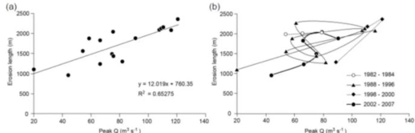
pressure, soil properties such as density or composition, and vegetative properties such as root depth and large woody debris affect bank stability. The factors that affect bank erosion are also affected by the scale of the research and the type of river. Variations in bank erosion rates among reaches of rivers of significantly different sizes have indicated that bank erosion rates increase with river size (e.g. width, discharge; Hooke, 1979). Studies of reaches of river migration with relatively constant discharge but with bends of varying morphology indicate a significant control of meander morphology (e.g. Nanson and Hickin, 1983). Studies of bank erosion along stretches of river in watersheds experiencing changes in discharge due to urbanization or other causes indicate both discharge and local characteristics affect bank erosion rates (e.g. Julian and Torres, 2006, Hooke, 2012). Hooke (2012) used historic (e.g. air photo data) to obtain bank erosion rates in a region with variable discharge. She found that the bank erosion rate for intervals correlated with peak discharge, with one of the main effects being the length of the bank area that eroded per measurements interval. An example of the relationship between discharge and erosion rates is shown in fig. 1.
3
Figure 1. Taken from Hooke 2012 showing the relationship between erosion length and peak discharge.
Part 2: Measurement of Bank Erosion Rates
Many techniques have been used to measure erosion rates, with different techniques used for different time scales, whether or not the river is meandering or braided, and how much
vegetation or debris there is in and around the river. A common approach for monitoring long term changes in bank erosion rates is the use of air photo time series as has been done by Hooke (2012). This method is a simple way of understanding the changing migration of a river through time, by taking air photos at multiple time intervals it is easier to see where and when certain places in the river erode more and therefore migrate at a faster rate. This procedure works best for sites where the bank is visible, i.e. in farmlands, grasslands and other locations where trees and other vegetation does not obscure the bank edge from the air. Similarly, direct channel measurements and resurveys are used to monitor erosion rates as well, however, the length of the monitoring period dates to the beginning of measurements. Measurements of this type are made at USGS gauging stations, but these gauges are often located along straight and relatively stable reaches. This process involves taking measurements of bank position and other morphological properties of the bank at sites along a reach of river, these measurements yield erosion rates in specific areas that allows for comparison between sites and therefore evaluation of differences which could increase or decrease erosion rate. Repeat LiDar surveys may also be used to determine channel morphology and its relationship with bank erosion (Pizzuto and Mecklenburg 2009).
Short-term, on the scale of storm events or portions of a year, erosion rates have been
monitored by a variety of methods. Bank erosion pins (Leopold and Maddock 1953) have been used in this type of measurement to be able to easily and quickly identify whether a bank is eroding, this is tested by simply inserting a pin or nail into the bank and checking periodically to measure how far the bank has eroded for a specific storm event or to check if it has been washed away due to the eroding bank not being able to hold it in place. This technique has been criticized because the erosion pins could cause local scour and enhance erosion, however, it still appears to be a very effective method with few drawbacks that actively hinder the
4
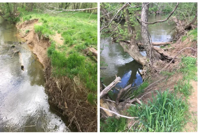
In addition to measurements of erosion rates, measurements of bank characteristics that might affect erosion rates can also been conducted. The root depth whether exposed or buried (due to bank erosion or overbank sedimentation respectively) plays an important role in determining the bank erosion in a specific area, the roots size and quantity within a bank work to prevent bank erosion by strengthening the structure of the bank and holding it in place (Pizzuto and Mecklenburg 2009, Malik 2006.).
Figure 2. A photo showing exposed roots along a section of the bank of Seneca Creek Part 3: Prediction Equations for Bank Erosion Rates
Many researchers have developed predictive equations that can be used to calculate bank erosion rates in rivers. These are largely empirical equations that predict erosion rate as a product of hydraulic effects, vegetative effects, or channel geometry. For example, Julian and Torres (2005) and Randle (2004) evaluated bank erosion rates based on hydraulic characteristics and bank vegetation characteristics. Many other researchers, e.g. Duan (2005), base their predictive equations on stream hydraulic and morphological characteristics. Hickin and Nanson (1983) generated a bank migration equation based on meander bend characteristics. These predictive equations are likely best used for sites with conditions similar to those for which they were developed.
The problem with all of these methods is that these erosion rate predictions may not account for many other river properties that have a significant effect on whether a bank will erode, therefore causing any erosion rate calculated to only be useful for one river or even one site in one river.
5
There are several predictive equations that include many parameters that vary along a river or among rivers. An example of this type of equation is that by Randle (2004), which expresses erosion rate as a function of factors that increase erosion rates (meander bend characteristics, velocity) and decrease erosion rates by affecting local bank strength (rooting density, morphology, woody debris, etc.).
𝐵𝑒 = {[𝑎1𝐶𝑠 (𝑊𝑏 𝑅𝑐)] − [𝑎2 (𝑅𝑦 ∗ 𝑅𝑑 𝐻𝑏) + 𝑎3 (𝐿𝑊𝐷 ∗ 𝑑𝑤 𝐷 ) + 𝑎4(𝑃𝐼) + 𝑎5 (𝑑𝑐 ∗ 𝐻𝑏 𝐷 )]} 𝑎6 ∗ 𝑉 Equation 1.
where Be = bank erosion rate, Cs = bed sediment concentration, Wb = bankfull channel width, Rc = channel radius of curvature, Ry = fraction of bank covered by vegetation roots, Rd =
vegetation root depth, Hb = bank height, LWD = fraction of bank covered by tree of large woody debris, Dw = average height of large woody debris jams, D = hydraulic depth of channel, PI = plastic index, Dc = portion of bank sediment too coarse for incipient motion, V = mean channel velocity [L/T], and a1 and a6 are empirical coefficients and a2, a3, a4, and a5 are weighting factors.
In the scope of my research I used this bank erosion equation as a guide to the factors that might influence bank erosion rates at my study site. The Randle bank erosion rate equation incorporates many of the river characteristics that have been previously shown to influence bank erosion that are consistent with the characteristics of the study site. These characteristics include river velocity, bend morphology, channel depth, width, rooting depth, root density, and amount/size of woody debris covering banks. I have also measured spatial variations in long-term erosion rates by analyzing short-long-term erosion rates by making repeated measurements along the channel bank.
Hypothesis
1) The increase in annual peak discharge at the USGS gauge on Seneca Creek is associated with significant channel widening (bank erosion) for the period 1938 to 2018.
2) Bank erosion rates measured from air photos (decadal time scales) increase with (Rc/w) ratio; they are highest on the outside of bends, where velocities are the highest.
3) Short-term erosion rates (measured after flood events) are highest during hydrographs that generated high velocities (and excess shear stress).
4) In the selected study reach rooting depths and bank vegetation protect the bank from erosion and therefore are inversely correlated with local bank erosion rates measured by air photos or erosion pins.
These hypotheses were developed by building off the previous research to suggest that bank erosion rate is affected by hydraulic effects (water velocity, river width, river discharge) in the
6
long term and throughout the entire river. Local variations in bank erosion rate along a reach of river within shorter time periods is due to heterogeneities of vegetation or rooting depth. The idea behind this is that the hydraulic effects act as an amplifier or reducer to the overall erosion rate of the river while vegetative effects along a reach of river act as buffer between the bank and the water to reduce the rate of erosion in specific areas. As a result, what would occur is that along a reach of river there are varying rates of erosion that can be monitored with different techniques and predicted from measuring the properties of the river at specific sites along said reach.
Study Site and Methods
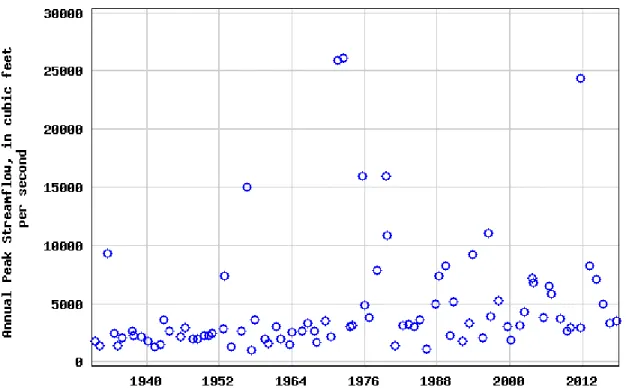
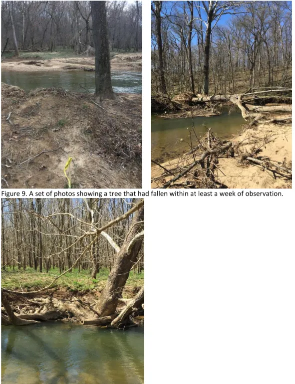
The study site is a section of Seneca Creek near Dawsonville, Maryland (fig. 3). The site is located upstream of a USGS gauging station. The Seneca Creek watershed contains rapidly suburbanizing areas in Rockville and Gaithersburg, Maryland. As a result, peak discharges in the watershed have been increasing over the past few decades (fig. 4). Examination of the field site indicates high rates of bank erosion (exposed roots, fallen trees, etc.) as well as overbank deposition of coarse sand. During the observation period, I monitored bank erosion that undermined the root structure of a tree (fig 9), which suggests that bank erosion is an active process as whole in this river and specifically in the chosen study area.
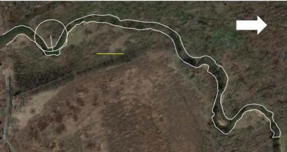
Figure 3. An air-photo of the study area along Seneca Creek. The superimposed yellow bar represents 100 meters length, the superimposed white arrow represents north direction. The superimposed circle shows the radius of curvature for one of the meander bends.
7
Part 1: Temporal Variations in Discharge and Channel Morphology through USGS Gauge Data USGS Hydraulic Data
Hydraulic data, consisting of river width and depth, velocity, and discharge is available for the period from 1938 to the present. In addition to the peak discharge data, stream measurement data was also be acquired. These data was divided into 10-year increments and used to
determine annual average peak discharge, and maximum peak discharge. This approach is similar to the approach taken by Hooke (2009), who used gauge data to obtain average flood discharge values for time increments for which she obtained channel change data.
Air photos of Seneca Creek show the general trace of the channel banks, but the actual bank edge is often covered by trees (fig. 3). Therefore, in addition to the annual peak discharge data, the USGS stream measurement data was used to obtain bankfull channel morphology and velocity data by evaluating the at-a-station hydraulic geometry for each 10-year period. The hydraulic geometry relationships are the power function relationships between discharge and width, depth and velocity at a given station (Leopold and Maddock, 1953). The at-a-station hydraulic geometry equations refer to in-bank flows:
W = aQb , D = cQf , V = kQm
where Q = discharge, w = channel surface width, D = average depth (Area/W), and V = average velocity. Due to continuity, W*D*V = Q; therefore b+f+m = 1.0 and a*c*k = 1.0
An example of Hydraulic Geometry relationships for the time period 1949-1958 is shown in figure 5.
8
Figure 5. These graphs are an example of the hydraulic geometry relationships taken from USGS gauge data for the years 1949 to 1958.). Bankfull discharge can be identified most clearly on the width versus discharge diagram, which indicates a large increase in width (from 165 feet to 540 feet) for a small change in discharge (1800 to 2,000 cfs) as the channel overtops its bank and uses the floodplain to carry part of the discharge.
The width for the mean annual peak Q was calculated from these hydraulic geometry relationships for each time interval. Similarly, the hydraulic geometry data was used to
calculate the discharge, width, depth, and velocity for bankfull flows in each 10-year period (see table 1). Bankfull discharge is commonly the 1.5 year R.I. (Recurrence Interval) discharge, so it will likely be lower than the average annual peak discharge in each time interval.
Table 1: Discharge Data for time intervals
Interval Ave Annual Peak
Discharge, Q, cfs Maximum Q, cfs Bankfull Q, cfs ~1.5-year RI Velocity for Bankfull Q 1939 – 1948 2062 3620 1810 3.05 1949 – 1958 2838 15000 503 3.75 1959 – 1968 2167 3070 373 3.25 1969 - 1978 7805 26100 228 2.09 1979 - 1988 4647 16000 310 2.77 1989 - 1998 4571 11000 209 1.82 1999 - 2008 4329 7130 3610 4.13 2009 - 2018 4448 24400 3120 2.99
9
In summary, from these USGS hydraulic data, the following information for the 10-year increments has been obtained: average annual peak, Maximum peak Q, and the bankfull characteristics, and the associated bankfull width, depth, and velocity. These data could be used in bank erosion rate predictive equations, which often incorporate discharge and velocity.
Analysis of change and association with discharge
I have evaluated the changes in bankfull channel characteristics at the USGS gauge by
determining the bankfull characteristics of each time interval and using these data to determine channel changes between each 10 –year interval. Channel widening is bank erosion, which would be indicated by a positive width/year. Similarly, an increase in depth would be a positive change in channel depth as depth/year.
Hooke (2012) found a simple relationship between annual bank erosion rate and maximum discharge:
I examined the hydraulic and channel change data to determine whether similarly simple relationships between channel width enlargement rate (bank erosion rate) and discharge exist. It is also possible that the channel will enlarge due to increases in channel depth (due to
overbank sedimentation, channel incision, or both) rather than increases in channel width.
Part 2: Spatial Variation in Channel Morphology through Long-term and Short-term Bank Erosion Measurements.
The first part of my study used USGS gauging station data. These data extend over a significant period of time, but only provide information about one cross section of the river. In this part of my study, I examined spatial differences in bank erosion rates, and associated variations in channel morphology and bank characteristics. For this part of my study, I have selected 8 areas along of a reach of Seneca Creek (fig. 6).
10
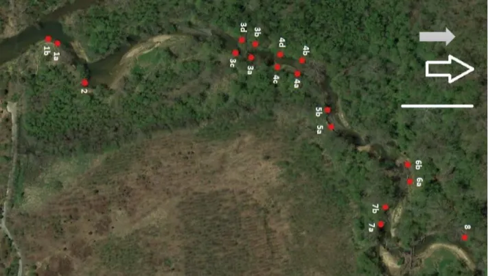
Figure 6. Air photo of the study area displaying where specific sites for measurements are located. The superimposed white bar represents 100 meters on the ground and the white arrow is north direction.
These reaches of river were selected to provide a range of planform morphology ranging from tight meander bends (Rc of 20.12 m) to open meander bends (Rc of 29.67 m) to straight reaches (table 2). For these selected reaches, migration rate was estimated by measuring the changes in channel area for each segment divided by the segment length for the 4/2008 and 4/2018 air photos (which were the best resolution and taken during dormant periods for vegetation). These migration amounts were divided by the time interval (10 years) to obtain migration rate. Examples of channel changes between the 2008 and 2018 channels on the air photos are shown in fig. 7.
11
Fig. 7: Channel Boundaries from the 4/2008 channel shown on the 4/2018 image (drawn in Google Earth, the image is from the USGS for both years, the orange arrow is north direction). Note the cut-off chute that was formed and subsequently reconnected in the middle of the bank.
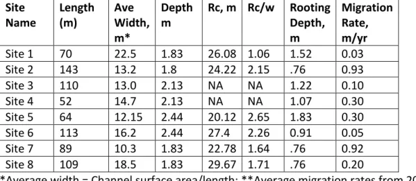
Table 2: Physical Characteristics of the channel of study reaches and associated migration rates
Site Name Length (m) Ave Width, m* Depth m Rc, m Rc/w Rooting Depth, m Migration Rate, m/yr Site 1 70 22.5 1.83 26.08 1.06 1.52 0.03 Site 2 143 13.2 1.8 24.22 2.15 .76 0.93 Site 3 110 13.0 2.13 NA NA 1.22 0.10 Site 4 52 14.7 2.13 NA NA 1.07 0.30 Site 5 64 12.15 2.44 20.12 2.65 1.83 0.30 Site 6 113 16.2 2.44 27.4 2.26 0.91 0.05 Site 7 89 10.3 1.83 22.78 1.64 .76 0.92 Site 8 109 18.5 1.83 29.67 1.71 .76 0.20
*Average width = Channel surface area/length; **Average migration rates from 2008 and 2018 air photos calculated as surface area change per unit length divided by time interval.
12
Short-Term Bank Erosion and Overbank Sedimentation Rates
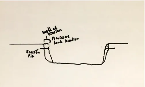
The 2016 and 2018 air photos indicate that large amounts of woody debris entered the channel after 2016. This debris may have an impact on the amount and location of future bank erosion rates. Therefore, the last set of data that I have collected throughout the year is the actual bank migration through short intervals of time. This was measured through the year after major storm events. These measurements were made at installations near the bank. The process for this was inserting erosion pins flush with the bank at each station along the river (figure 6.) to monitor bank erosion. After storm events the bank will erode inward, leaving the pin behind as a record of where the bank used to be thus yielding erosion data; an example of this method is shown in figure 8.
Figure 8. A diagram of the aforementioned erosion pin method.
I have taken reliable measurements on the bank migration and other parameters (such as large river discharge and rooting depths) throughout the year. Throughout the year I have visited the study area many times and there were noticeable changes in the properties along the bank each time. These properties include overhanging banks, exposed roots, fallen trees and slumped banks. These examples of changing river morphology and spatial variations in vegetation all indicate that the river is actively eroding. The error associated with these measurements arise from innate uncertainty in measuring tools i.e. tape measures, google earth satellite accuracy, USGS gauge sites. The percent error in google earth polygon and line measurements is 3.54% and 0.44% respectively (Nogueira and Lopes 2011). The USGS gauge data is accurate to 2%-5%. The tape measure that I am using is accurate to + 0.1cm.
13
Figure 9. A set of photos showing a tree that had fallen within at least a week of observation.
Figure 10. A photo showing the exposed root systems of a tree that had been growing on a bank that has since eroded inland.
14
Results
Temporal Data
Table 2 shows the physical characteristics of the channel in the study reach. The width of the study reach did not vary significantly but the radius of curvature did. I measured the radius of curvature for each bend five times to obtain errors for each site, table 4 shows this the results below.
Table 4: Physical Characteristics of the channel of study reaches and associated migration rates
Site Name Length (m) Ave Width, m* Depth m Rc, m Rc/w Rooting Depth, m Migration Rate, m/yr Site 1 70 22.5 1.83 26.08 1.06 1.52 0.03 Site 2 143 13.2 1.8 24.22 2.15 .76 0.93 Site 3 110 13.0 2.13 NA NA 1.22 0.10 Site 4 52 14.7 2.13 NA NA 1.07 0.30 Site 5 64 12.15 2.44 20.12 2.65 1.83 0.30 Site 6 113 16.2 2.44 27.4 2.26 0.91 0.05 Site 7 89 10.3 1.83 22.78 1.64 .76 0.92 Site 8 109 18.5 1.83 29.67 1.71 .76 0.20
*Average width = Channel surface area/length; **Average migration rates from 2008 and 2018 air photos calculated as surface area change per unit length divided by time interval.
Table 5. The average and standard deviation of radius of curvature measurements.
The hydraulic geometry equations were used to calculate the peak velocity for the maximum discharge for each time interval, specifically, the discharge versus velocity graph. Doing this allowed showed that intervals with high discharges exhibit higher velocities and as a result greater rates of erosion for the time interval. Table 5 shows the erosion pin data and their association with velocity and discharge.
15
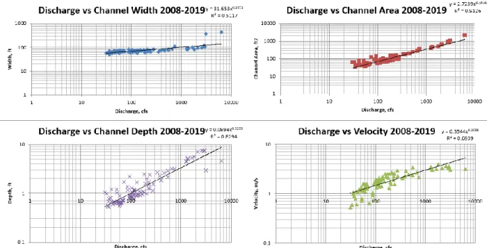
Figure 11. These graphs are an example of the hydraulic geometry relationships taken from USGS gauge data for the years 2008 to 2019.). Bankfull discharge can be identified most clearly on the width versus discharge diagram, which indicates a large increase in width (from 165 feet to 540 feet) for a small change in discharge (1800 to 2,000 cfs) as the channel overtops its bank and uses the floodplain to carry part of the discharge.
Erosion Pin Data (Short Term Event Data)
Erosion pin data was collected over five time intervals from August to November. Figure 12 shows the associated discharges for each of these events and table 5 displays the erosion pin data for each of these time intervals.
Figure 12. The Discharge hydrograph for the period of July 25th to November 5th during which time the erosion pin data were collected.
16
Below are the erosion pin data for the five time intervals over which I measured erosion and the
associated discharge and velocity values. The erosion data for each time interval shows that the erosion is approximately 1 cm or more, the relationship between peak velocity and erosion is shown in figure 13.
Table 5. Showing the erosion pin data with associated discharge and velocity values.
Figure 13. Showing the relationship between velocity and amount of erosion.
Spatial Variation in Erosion Rates From 2008 to 2018 Air Photo Data
Table 2 shows significant variations in erosion rates among the eight channel reaches. This section will examine the erosion rates to the characteristics of each of the reaches. The first figure below shows migration rate versus rooting depth, the second figure below shows the migration rate versus radius of curvature to width ratio.
y = 0.324x + 1.333 R² = 0.4414 0.0 0.5 1.0 1.5 2.0 2.5 3.0 3.5 0.0 0.5 1.0 1.5 2.0 2.5 3.0 3.5 4.0 4.5 Ero sion , cm Velocity, m/s
Erosion vs Velocty
17
Figure 14. Shows the relationship between migration rate and rooting depths at each site.
Figure 15. Showing the exposed roots of a tree and the eroded bank behind it.
There is a variation in migration rate at each site. While most sites have low migration rate across rooting depths there are several sites where migration rate is high at low rooting depths. This suggests that rooting depth by itself was not a major control on migration rates.
0 0.2 0.4 0.6 0.8 1 0.0 0.2 0.4 0.6 0.8 1.0 M ig ra ti o n r ate, m /y ea r
Rooting depth/Channel Depth
Migration Rate versus Rooting
Depth/Channel Depth
18
Figure 16. Shows migration rate versus radius of curvature to width ratios.
The highest migration rates were found to be around radius of curvature to widths of about 2.3.
Discussion and Conclusion
Using the Randle equation as a guide I evaluated the importance of the parameters associated with erosion rate. Many of the parameters were found not to be very useful within a reach, rather than among reaches. Some of these parameters were: Rooting depth, large woody debris, the height of debris jams, and bed sediment concentration. This is because the banks of the study reach had a consistent sediment make-up of clay/silt along the lower half to a coarse sand on top that were consistent throughout the reach. The debris did not have an effect on the erosion rates because there was either no large woody debris present or the velocities were high enough to wash them away. Rooting depth was found not to be strongly correlated with erosion rate as stated above since we see that migration rates vary significantly across varying rooting depths. What I did find was that velocity and radius of curvature are more important within this reach, both were observed to affect the erosion rates significantly as shown above. Velocity increases erosion rate and during the study there were multiple storm time intervals that exhibited different velocities with their individual erosion amounts varying as well (Table 3.), velocity has been increasing in this area through time due to urbanization. The radius of curvature to width ratio was also found to be an important factor that controls erosion rate. This is similar to the findings of Hicken and Nanson (1983), in which they found that radius of curvatures from 2 to 3 had the highest migration rates, which is also similar to what is shown in figure 14. Observationally there were many mass wasting events in which the bank slid into the
0 0.2 0.4 0.6 0.8 1 0 5 10 15 20 M ig ration R ate , m /y e ar
Rc/W
Migration Rate versus Radius of
Curvature to Width Ratio
19
river as it was undercut by high velocity water, these events usually happened in bends and were seen mostly after larger storms (figure 17).
Figure 16. Showing the Migration rate versus radius of curvature to width distribution from Hicken and Nanson 1983.
Figure 17. Showing a mass wasting event in which a section of bank slid into the river.
20
Duan, J.G., (2005), Analytical Approach to Calculate Rate of Bank Erosion: Journal of Hydraulic Engineering, v. 131, p. 980–990, doi: 10.1061/(asce)0733-9429(2005)131:11(980).
Edésio, Msc & Elias Lopes, Edésio & Ruth, Dra & Nogueira, Ruth. (2011). Proposta Metodológica para Validação de Imagens de Alta Resolução do Google Earth para a Produção de Mapas. Hooke, J. (2012). Dynamics of bank erosion on the River Dane, England. IAHS-AISH Publication. 356.
57-64.
Hooke, J., (1979), An analysis of the processes of river bank erosion: Journal of Hydrology, v. 42, p. 39–62, doi: 10.1016/0022-1694(79)90005-2.
Jerolmack, D.J., and Mohrig, D., (2007), Conditions for branching in depositional rivers: Geology, v. 35, p. 463, doi: 10.1130/g23308a.1.
Julian, J.P., and Torres, R., (2006), Hydraulic erosion of cohesive riverbanks: Geomorphology, v. 76, p. 193–206, doi: 10.1016/j.geomorph.2005.11.003.
Leopold, L.B., and Maddock, T., (1953), The hydraulic geometry of stream channels and some physiographic implications: Professional Paper, doi: 10.3133/pp252.
Malik, I., (2006), Contribution to understanding the historical evolution of meandering rivers using dendrochronological methods: example of the Mała Panew River in southern Poland: Earth Surface Processes and Landforms, v. 31, p. 1227–1245, doi: 10.1002/esp.1331.
Nanson, G.C., and Hickin, E.J., (1983), Channel Migration and Incision on the Beatton River: Journal of Hydraulic Engineering, v. 109, p. 327–337, doi: 10.1061/(asce)0733-9429(1983)109:3(327). Pizzuto, J.E., and Mecklenburg, T.S., (1989), Evaluation of a linear bank erosion equation: Water
Resources Research, v. 25, p. 1005–1013, doi: 10.1029/wr025i005p01005.
Pizzuto, J., (2009), An empirical model of event scale cohesive bank profile evolution: Earth Surface Processes and Landforms, v. 34, p. 1234–1244, doi: 10.1002/esp.1808.
Randle, T.J., (2004), Channel Migration Model for Meandering Rivers, p. 241–248.
Simon, A., Pollen-Bankhead, N., and Thomas, R.E., (2013), Development and Application of a Deterministic Bank Stability and Toe Erosion Model for Stream Restoration: Stream Restoration in Dynamic Fluvial Systems Geophysical Monograph Series, p. 453–474, doi:
10.1029/2010gm001006.
21 Decadal Max Gage # Date Q, cfs Q, cfs USGS 1645000 7/1/1931 1730 USGS 1645000 3/28/1932 1380 USGS 1645000 8/24/1933 9300 USGS 1645000 9/17/1934 2410 USGS 1645000 5/7/1935 1420 USGS 1645000 1/3/1936 2020 USGS 1645000 8/27/1937 2610 AVE 1928 USGS 1645000 10/23/1937 2280 USGS 1645000 1/30/1939 2150 USGS 1645000 4/20/1940 1740 USGS 1645000 6/23/1941 1300 USGS 1645000 5/22/1942 1460 USGS 1645000 10/16/1942 3620 USGS 1645000 11/9/1943 2660 USGS 1645000 8/1/1945 2110 USGS 1645000 6/2/1946 2940 USGS 1645000 8/20/1947 1990 USGS 1645000 6/30/1948 1990 AVE 2062 USGS 1645000 7/16/1949 2240 USGS 1645000 3/23/1950 2280 USGS 1645000 12/4/1950 2420 USGS 1645000 9/1/1952 2810 USGS 1645000 11/22/1952 7330 USGS 1645000 12/14/1953 1240 USGS 1645000 8/13/1955 2620 USGS 1645000 7/21/1956 15000 USGS 1645000 4/5/1957 959 USGS 1645000 12/21/1957 3640 AVE 2838 USGS 1645000 8/8/1959 1970 USGS 1645000 2/19/1960 1600 USGS 1645000 6/10/1961 3070 3070 USGS 1645000 3/12/1962 1920
22 USGS 1645000 8/20/1963 1480 USGS 1645000 1/9/1964 2520 USGS 1645000 8/26/1965 2640 USGS 1645000 9/14/1966 USGS 1645000 8/27/1967 2660 USGS 1645000 1/14/1968 1640 AVE 2167 USGS 1645000 9/4/1969 3490 USGS 1645000 7/10/1970 2200 USGS 1645000 9/12/1971 25900 USGS 1645000 6/22/1972 26100 USGS 1645000 9/14/1973 3020 USGS 1645000 12/26/1973 3160 USGS 1645000 9/26/1975 16000 USGS 1645000 1/1/1976 4900 USGS 1645000 10/9/1976 3770 AVE 7805 USGS 1645000 1/26/1978 7850 USGS 1645000 9/6/1979 16000 USGS 1645000 10/1/1979 10800 USGS 1645000 2/11/1981 1340 USGS 1645000 6/13/1982 3160 USGS 1645000 4/10/1983 3260 USGS 1645000 3/29/1984 3010 USGS 1645000 2/12/1985 3620 USGS 1645000 4/16/1986 1070 USGS 1645000 9/9/1987 4950 USGS 1645000 5/19/1988 7410 4647 USGS 1645000 5/6/1989 8250 USGS 1645000 4/2/1990 2270 USGS 1645000 10/23/1990 5120 USGS 1645000 3/27/1992 1750 USGS 1645000 4/16/1993 3350 USGS 1645000 11/28/1993 9160 USGS 1645000 8/6/1995 2080 USGS 1645000 6/18/1996 11000 USGS 1645000 10/19/1996 3880
23 USGS 1645000 3/21/1998 5280 AVE 4571 USGS 1645000 9/16/1999 3060 USGS 1645000 3/22/2000 1910 USGS 1645000 8/12/2001 3140 USGS 1645000 5/27/2002 4310 USGS 1645000 9/23/2003 7130 USGS 1645000 12/11/2003 6810 USGS 1645000 7/8/2005 3750 USGS 1645000 6/26/2006 6530 USGS 1645000 11/17/2006 5790 USGS 1645000 5/12/2008 3660 AVE 4329 USGS 1645000 5/26/2009 2650 USGS 1645000 12/26/2009 2930 USGS 1645000 9/8/2011 24400 USGS 1645000 10/13/2011 2890 USGS 1645000 1/31/2013 8280 USGS 1645000 5/16/2014 7040 USGS 1645000 6/28/2015 4950 USGS 1645000 7/31/2016 3350 USGS 1645000 7/29/2017 3490 AVE 4448
Decadal Discharge Summary
Decade Qmean Qmax
1935 1928 9300 1945 2062 3620 1955 2837 15000 1965 2166 3270 1975 7805 26100 1985 4647 16000 1995 4571 11000 2005 4328 7130 2015 4448 24400
24
Appendix II: USGS gauging station data for 1949-1958 Channel Discharge Channel Width Channel Velocity Channel Depth 238 55 3.42 1.267272727 211 53 3.13 1.271698113 237 56 3.44 1.244642857 155 72 2.75 0.783333333 112 47 2.06 1.157446809 112 48.5 2 1.156701031 106 47 1.97 1.144680851 62.8 52.5 1.5 0.794285714 73.5 46 1.53 1.045652174 54.8 50.5 1.51 0.720792079 43.3 46 1.16 0.813043478 343 65.5 3.36 1.557251908 73.8 45 1.6 1.035555556 85.9 47 1.8 1.014893617 92.2 49 1.71 1.1 89.2 52.5 1.52 1.12 133 64 2.51 0.828125 114 51.8 2.41 0.913127413 96.4 53 1.99 0.911320755 66.9 46.5 1.51 0.95483871 51.1 45 1.33 0.851111111 32.9 50 1.3 0.506 41.2 50 1.33 0.62 51.2 45 1.33 0.855555556 56.2 47 1.46 0.819148936 82.4 45.5 1.75 1.032967033 160 53.6 2.49 1.199626866 100 53 2.04 0.922641509 261 87 3.14 0.954022989 131 45 2.17 1.342222222 129 64 2.6 0.978125 163 70 2.73 0.854285714 70.2 53.5 1.87 0.702803738 216 68 2.78 1.141176471 71.9 49.5 1.45 1.004040404 34.7 42 0.89 0.928571429 26.8 46.5 0.89 0.64516129 28.9 44 0.74 0.886363636 48.2 50 1.1 0.87 244 54 2.74 1.646296296 75.8 47.5 1.32 1.208421053 50.2 54 1.25 0.744444444
25 45.5 48.5 0.4 1.039175258 144 47.5 2.17 1.4 501 47 1.09 1.170212766 56.8 52.5 1.75 0.619047619 46.7 46 1.21 0.841304348 41.8 49.5 0.83 1.022222222 42.9 47.5 0.87 1.035789474 242 68 3.21 1.108823529 81.6 53 2.14 0.720754717 136 52 1.89 1.380769231 321 55.5 2.89 2 503 72 3.75 1.861111111 106 47 1.67 1.35106383 1810 165 3.6 3.054545455 152 55 2 1.381818182 97.7 54.4 1.6 1.119485294 55.4 57.5 1.11 0.871304348 2680 2.21 2310 540 2.14 2 60 53 1.42 0.794339623 53 46 1.19 0.97173913 7330 107 66 2.11 0.783333333 114 54.5 1.45 1.44587156 115 51 1.57 1.435294118 158 54 1.8 1.622222222 60.1 53 1.26 0.9 43 53.5 0.86 0.940186916 27.9 27.5 1.43 0.709090909 42.5 41 1.08 0.96097561 65.3 42.5 1.4 1.101176471 80.3 42 1.62 1.178571429 41.4 53.5 1 0.771962617 13 19.6 1.09 0.607142857 10.2 20.5 0.91 0.546341463 27.5 30 1.16 0.79 25.8 26.2 1.07 0.923664122 59.8 45 1.2 1.104444444 22.3 26 1.18 0.726923077 8.19 23 0.65 0.547826087 34.9 34.5 1.63 0.620289855 34.7 34 1.48 0.688235294 47 35 1.71 0.785714286 29.4 28.5 1.3 0.792982456 107 68 2.06 0.764705882 94.4 51 1.57 1.178431373
26 47.4 34.5 1.72 0.8 60.4 44 1.38 0.997727273 103 41 2.38 1.056097561 61.7 33 1.88 0.996969697 179 60 2.48 1.201666667 75.7 54 1.53 0.918518519 28.6 28 1.3 0.842857143 13.7 38 1.75 0.062631579 16 47 0.47 0.744680851 15.9 25 0.89 0.72 174 65 2.44 1.107692308 88.2 49.5 1.68 1.060606061 67.9 33 1.55 1.324242424 26.4 72 2.69 1.359722222 83.6 50 1.61 1.036 133 54 2 1.231481481 56.2 53 1.53 0.69245283 45.8 51 0.91 0.982352941