Galaxy and Mass Assembly (GAMA): ugriz galaxy luminosity functions

Galaxy and Mass Assembly (GAMA):

ugriz

galaxy luminosity

functions

J. Loveday,

P. Norberg,

I.K. Baldry,

S.P. Driver,

A.M. Hopkins,

J.A. Peacock,

S.P. Bamford,

J. Liske,

J. Bland-Hawthorn,

S. Brough,

M.J.I. Brown,

E. Cameron,

C.J. Conselice,

S.M. Croom,

C.S. Frenk,

M. Gunawardhana,

D.T. Hill,

D.H. Jones,

L.S. Kelvin,

K. Kuijken,

R.C. Nichol,

H.R. Parkinson,

S. Phillipps,

K.A. Pimbblet,

C.C. Popescu,

M. Prescott,

A.S.G. Robotham,

R.G. Sharp,

W.J. Sutherland,

E.N. Taylor,

D. Thomas,

R.J. Tuffs,

E. van Kampen,

D. Wijesinghe

1_{Astronomy Centre, University of Sussex, Falmer, Brighton BN1 9QH, UK}

2_{Institute for Astronomy, University of Edinburgh, Royal Observatory, Blackford Hill, Edinburgh EH9 3HJ, UK}

3_{Institute for Computational Cosmology, Department of Physics, Durham University, South Road, Durham DH1 3LE, UK}

4_{Astrophysics Research Institute, Liverpool John Moores University, Twelve Quays House, Egerton Wharf, Birkenhead, CH41 1LD, UK} 5_{School of Physics & Astronomy, University of St Andrews, North Haugh, St Andrews, KY16 9SS, UK}

6_{International Centre for Radio Astronomy Research (ICRAR), The University of Western Australia, 35 Stirling Highway, Crawley, WA6009, Australia} 7_{Australian Astronomical Observatory, PO Box 296, Epping, NSW 1710, Australia}

8_{Centre for Astronomy and Particle Theory, University of Nottingham, University Park, Nottingham NG7 2RD, UK} 9_{European Southern Observatory, Karl-Schwarzschild-Str. 2, 85748 Garching, Germany}

10_{Sydney Institute for Astronomy, School of Physics, University of Sydney, NSW 2006, Australia} 11_{School of Physics, Monash University, Clayton, Victoria 3800, Australia}

12_{Department of Physics, Swiss Federal Institute of Technology (ETH-Z¨urich), 8093 Z¨urich, Switzerland} 13_{Leiden University, P.O. Box 9500, 2300 RA Leiden, The Netherlands}

14_{Institute of Cosmology and Gravitation (ICG), University of Portsmouth, Dennis Sciama Building, Burnaby Road, Portsmouth PO1 3FX, UK} 15_{Astrophysics Group, HH Wills Physics Laboratory, University of Bristol, Tyndall Avenue, Bristol BS8 1TL}

16_{Jeremiah Horrocks Institute, University of Central Lancashire, Preston PR1 2HE, UK}

17_{Research School of Astronomy & Astrophysics, The Australian National University, Cotter Road, Weston Creek, ACT 2611, Australia} 18_{Astronomy Unit, Queen Mary University London, Mile End Rd, London E1 4NS, UK}

19_{Max Planck Institute for Nuclear Physics (MPIK), Saupfercheckweg 1, 69117 Heidelberg, Germany}

25 October 2018

ABSTRACT

Galaxy and Mass Assembly (GAMA) is a project to study galaxy formation and evolution, combining imaging data from ultraviolet to radio with spectroscopic data from the AAOmega spectrograph on the Anglo-Australian Telescope. Using data from phase 1 of GAMA, taken over three observing seasons, and correcting for various minor sources of incompleteness, we calculate galaxy luminosity functions (LFs) and their evolution in theugrizpassbands.

At low redshift,z < 0.1, we find that blue galaxies, defined according to a magnitude-dependent but non-evolving colour cut, are reasonably well fitted over a range of more than ten magnitudes by simple Schechter functions in all bands. Red galaxies, and the combined blue-plus-red sample, require double power-law Schechter functions to fit a dip in their LF faintwards of the characteristic magnitudeM∗before a steepening faint end. This upturn is at least partly due to dust-reddened disc galaxies.

We measure evolution of the galaxy LF over the redshift range0.002< z <0.5both by using a parametric fit and by measuring binned LFs in redshift slices. The characteristic lumi-nosityL∗is found to increase with redshift in all bands, with red galaxies showing stronger luminosity evolution than blue galaxies. The comoving number density of blue galaxies in-creases with redshift, while that of red galaxies dein-creases, consistent with prevailing

move-? _{E-mail: [email protected]}

ment from blue cloud to red sequence. As well as being more numerous at higher redshift, blue galaxies also dominate the overall luminosity density beyond redshiftsz'0.2. At lower redshifts, the luminosity density is dominated by red galaxies in therizbands, by blue galax-ies inuandg.

Key words: galaxies: evolution — galaxies: luminosity function, mass function — galaxies:

statistics.

1 INTRODUCTION

Measurements of the galaxy luminosity function (LF) and its evolu-tion provide important constraints on theories of galaxy formaevolu-tion and evolution, (see e.g. Benson et al. 2003). It is currently believed that galaxies formed hierarchically from the merger of sub-clumps. Looking back in time with increasing redshift, the star formation rate appears to peak at redshiftz'1, above which it plateaus and slowly declines towardsz ' 6(Cole et al. 2000; Hopkins 2004; Hopkins & Beacom 2006; Yuksel et al. 2008; Kistler et al. 2009). Sincez ' 1, galaxies are thought to have evolved mostly pas-sively as their stellar populations age, with occasional activity trig-gered by accretion and interactions with other galaxies. Noeske et al. (2007) have suggested that the first major burst of star formation is delayed to later times for low mass galaxies, contributing to the downsizing phenomenon.

There has long been a discrepancy between the measured number density of low-luminosity galaxies (the ‘faint end’ of the LF) and predictions from cold dark matter (CDM) hierarchical sim-ulations, in the sense that fewer low-luminosity galaxies than pre-dicted by most models are observed (Trentham & Tully 2002). Of course, interpretation of these simulation results is subject to un-certainties in the baryon physics. In particular, more effective feed-back in low mass halos might act to suppress the faint end of the LF. However, it is also possible that many surveys have underesti-mated the number of dwarf galaxies due to the correlation between luminosity and surface brightness which makes them hard to de-tect (Driver 1999; Cross & Driver 2002; Cameron & Driver 2007, 2009). Geller et al. (2011) have recently demonstrated that the LF faint-end slope steepens with decreasing surface brightness.

Galaxy LFs have previously been measured in the ugriz

bands from the Sloan Digital Sky Survey (SDSS, York et al. 2000) by Blanton et al. (2003b), Loveday (2004), Blanton et al. (2005b), Montero-Dorta & Prada (2009), and Hill et al. (2010). Blanton et al. (2003b) analysed a sample of 147,986 galaxies, roughly equiv-alent to SDSS Data Release 1 (DR1, Abazajian et al. 2003). They fit the LF with a series of overlapping Gaussian functions, allowing the amplitude of each Gaussian to vary, along with two parameters

Qand P describing, respectively, luminosity and density evolu-tion. They maximized the joint likelihood of absolute magnitude and redshift, rather than the likelihood of absolute magnitude given redshift, making this estimator more sensitive to evolution, as well as to density fluctuations due to large-scale structure. They found luminosity densities atz= 0.1to increase systematically with ef-fective wavelength of survey band, and for luminosity evolution to decline systematically with wavelength. Allowing for LF evo-lution enabled reconciliation of previously discrepant luminosity densities obtained from SDSS commissioning data (Blanton et al. 2001) and the Two-degree field Galaxy Redshift Survey (Folkes et al. 1999; Norberg et al. 2002).

Loveday (2004) measured the r-band LF in redshift slices from SDSS DR1 and found that the comoving number density of

galaxies brighter thanMr−5 lgh=−21.5mag was a factor'3

higher at redshiftz = 0.3than today, due to luminosity and/or density evolution.

Blanton et al. (2005b) focused on the faint end of the LF of low-redshift galaxies from SDSS DR2 (Abazajian et al. 2004), and found that a double-power-law Schechter function was required to fit an upturn in the LF atMr −5 lgh >_{∼ −}18mag with

faint-end slopeα2 ' −1.5after correcting for low surface-brightness

incompleteness.

Montero-Dorta & Prada (2009) have analysed SDSS DR6 (Adelman-McCarthy et al. 2008) which is roughly five times larger than the sample analysed by Blanton et al. (2003b). Their results are generally consistent with those of Blanton et al., although they do point out a bright-end excess above Schechter function fits, par-ticularly in theuandgbands, due primarily to active galactic nuclei (AGNs). A bright-end excess above a best-fitting Schechter func-tion has also been observed in near-IR passbands by Jones et al. (2006).

Hill et al. (2010) analysed combined datasets from the Millen-nium Galaxy Catalogue (Liske et al. 2003), SDSS and the UKIDSS Large Area Survey (Lawrence et al. 2007) over a common volume of'71,000h−3Mpc3within redshiftz= 0.1to obtain LFs in the

ugrizY J HKbands. They found that LFs in all bands were rea-sonably well fitted by Schechter functions, apart from tentative up-turns at the faint ends of thei- andz-band LFs. Hill et al. provided the first homogeneous measurement of the luminosity density (LD) over the optical–near-IR regimes, finding a smooth spectral energy distribution (SED).

Here we present an estimate ofugrizgalaxy LFs from the Galaxy and Mass Assembly (GAMA, Driver et al. 2009, 2011) survey. GAMA provides an ideal sample with which to constrain the galaxy LF at low to moderate redshifts due to its combination of moderately deep spectroscopic magnitude limit (r < 19.4or

r <19.8) and wide-area sky coverage (three4×12deg2regions). We describe the input galaxy sample and incompleteness, ve-locity andK-corrections in Section 2. Our LF estimation proce-dure is described in Section 3 and tested using simulations in Ap-pendix A. We present our results and a discussion of luminosity and density evolution in Section 4, with our conclusions summarized in Section 5.

Unless otherwise stated, we assume a Hubble constant of

H0= 100hkm/s/Mpc and anΩM = 0.3,ΩΛ= 0.7cosmology in

calculating distances, co-moving volumes and luminosities.

2 DATA AND OBSERVATIONS

2.1 Input catalogue

The input catalogue for GAMA is described in detail by Baldry et al. (2010). In brief, it consists of three4×12deg2 regions cen-tred approximately on the equator and at right ascensions of 9, 12

and 14.5 hours. These fields are known as G09, G12 and G15 re-spectively. Primary galaxy targets were selected from Data Release 6 (DR6, Adelman-McCarthy et al. 2008) of the Sloan Digital Sky Survey (SDSS, York et al. 2000) to extinction-corrected, Petrosian magnitude limits ofr <19.4mag in the G09 and G15 fields and

r <19.8mag in the G12 field.

We require Petrosian and model magnitudes and their errors in all five SDSS passbands in order to determineK-corrections (Sec-tion 2.5), and so we match objects in the GAMA team catalogue TilingCatv16 to objects in the SDSS DR6 PhotoObj table on SDSS ObjID using the SDSS CASJOBS1 service. We use only objects with GAMASURVEY CLASS≥ 3in order to exclude additional filler targets from the sample. We exclude objects, which, upon vi-sual inspection, showed no evidence of galaxy light, were not the main part of a deblended galaxy, or had compromised photometry (VIS CLASS= 2, 3 or 4 respectively). See Baldry et al. (2010) for further details of these target flags and Section 2.7 for a discussion of additional visual inspection of extreme luminosity objects.

In estimating LFs, we use Petrosian magnitudes corrected for Galactic extinction according to the dust maps of Schlegel, Finkbeiner, & Davis (1998). We make no attempt here to correct for intrinsic dust extinction within each galaxy, as was done by Driver et al. (2007), nor to extrapolate the Petrosian magnitudes to total, as done, for example, by Graham et al. (2005) and Hill et al. (2011). These systematic corrections to SDSS photometry, much more significant than any small random errors, will be considered in a subsequent paper.

An exception to our use of Petrosian magnitudes is foru-band data, where we instead use a pseudo-Petrosian magnitude defined by

upseudo−Petro=umodel−rmodel+rpetro. (1)

The reason for this is that the Petrosianu-band quantities are noisy and suffer from systematic sky-subtraction errors (Baldry et al. 2005). The pseudo-Petrosianu-band magnitude defined above, (us-ing the SDSSrband since it has highest signal-to-noise), and re-ferred to asuselectby Baldry et al. (2005), is much better behaved

at faint magnitudes.

For colour selection (see Section 2.6), we use SDSS model magnitudes in defining (g−r) colour, as recommended by the SDSS website2.

2.2 Spectroscopic observations

GAMA spectroscopic observations are described in the first GAMA data release paper (Driver et al. 2011). Observations for the GAMA Phase 1 campaign were made over 100 nights between 2008 February and 2010 May, comprising 493 overlapping two-degree fields. Redshifts were assigned in a semi-automated fashion by the observers at the telescope. A subsequent re-redshifting ex-ercise (Liske et al. in prep.) was used to assign a normalised qual-itynQto each redshift, according to each particular observer and their assigned qualityQ. Here we use reliable (nQ >2) redshifts from all three years of the GAMA Phase 1 campaign. In addi-tion to pre-existing redshifts and those obtained with the Anglo-Australian Telescope, twenty redshifts of brighter galaxies were obtained with the Liverpool Telescope. The GAMA-II campaign,

1 _{http://casjobs.sdss.org/CasJobs/}

2 _{http://www.sdss.org/dr7/algorithms/photometry.}

html

extending the survey to additional southern fields, began in 2011, but only GAMA-I redshifts are used here.

2.3 Completeness

Although GAMA has a very high spectroscopic completeness (> 98per cent; Driver et al. 2011), the small level of incompleteness is likely to preferentially affect low surface brightness, low luminos-ity galaxies, or galaxies lacking distinctive spectral features. We have identified three sources of incompleteness that potentially af-fect the survey: the completeness of the input catalogue (imaging completeness), completeness of the targets for which spectra have been obtained (target completeness) and the success rate of ob-taining spectroscopic redshifts (spectroscopic success rate). These three sources of incompleteness, and how we correct for them, are now considered in turn.

2.3.1 Imaging completeness

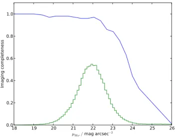
Imaging completeness has been estimated for the SDSS main galaxy sample by Blanton et al. (2005b), who passed fake galaxy images through the SDSS photometric pipeline. Blanton et al. found that imaging completeness is nearly independent of appar-ent magnitude (at least down tomr≈18mag), depending mostly

onr-band half-light surface brightness,µ50,r(their Fig. 2). Thus,

while GAMA goes about 2 mag fainter than the SDSS main galaxy sample, the Blanton et al. imaging completeness should still be ap-proximately applicable. We have used their imaging completeness estimates modified in the following ways3:

(i) Blanton et al. determine imaging completeness over the sur-face brightness range18< µ50,r < 24.5mag arcsec−2.

Extrap-olating their completeness as faint asµ50,r = 26mag arcsec−2

results in negative completeness values. We therefore arbitrarily as-sume 1 per cent imaging completeness atµ50,r= 26mag arcsec−2

and linearly interpolate from the faintest tabulated Blanton et al. completeness point at (µ50,r,fph) = (24.34, 0.33).

(ii) The Blanton et al. imaging completeness decreases at the bright end,µ50,r<_∼19mag arcsec−2, due to a lower angular size

limit of θ50 > 2 arcsec and a star-galaxy separation criterion ∆sg = rpsf−rmodel > 0.24for the SDSS main galaxy

sam-ple which excludes some compact, high surface-brightness (HSB) galaxies. GAMA target selection uses a far less stringent∆sg > 0.05, backed up byJ−Kcolour selection, and so is much more complete in HSB galaxies. We therefore omit the Blanton et al. completeness points atµ50,r<19.2mag arcsec−2and instead

as-sume 100 per cent completeness atµ50,r= 19.0mag arcsec−2and

brighter.

Our revised imaging completeness curve, along with a histogram ofµ50,rvalues for GAMA galaxies, is given in Fig.1.

3 _{An alternative way of estimating imaging completeness is to determine}

Figure 2.GAMA target completeness as a function of magnitude (pseudo-Petrosian foru, Petrosian forgriz). The upper panels show galaxy counts in varying-width magnitude bins, chosen to give roughly equal numbers of galaxies per bin, for GAMA targets (thin black histogram) and counts for galaxies that have been spectroscopically observed (thick red histogram). The lower panels show target completeness, ie. the ratio of observed to target counts, with the horizontal dotted line indicating 100 per cent target completeness. Vertical dashed lines indicate our chosen magnitude limits in each band: 20.3, 19.5, 19.4, 18.7, 18.2 inugrizrespectively.

18 19 20 21 22 23 24 25 26

µ50,r/ mag arcsec−2

0.0 0.2 0.4 0.6 0.8 1.0

Imaging completeness

Figure 1.Top line shows imaging completeness as a function ofr-band half-light surface brightness,µ50,r, from Blanton et al. (2005b),

modi-fied as described in the text. The histogram shows the normalised counts ofµ50,rfor galaxies in the GAMA sample.

2.3.2 Target completeness

Target completeness in therband may be assessed relative to the GAMA tiling catalogue, which contains all galaxies tor = 19.8

mag in the GAMA regions. In theugiz bands, however, there is no well-defined magnitude limit. We therefore re-implement the GAMA target selection criteria detailed by Baldry et al. (2010) on samples of objects selected from the SDSS DR6PHOTOOBJtable. We replace the Baldry et al. (2010) magnitude limits (their

equa-tion 6) with the following:u <21.0,g <20.5,r <20.0,i <19.5

orz <19.0.

Target completeness in each band is then simply defined as the fraction of target galaxies that have been spectroscopically ob-served, either by GAMA or by another redshift survey, as a func-tion of apparent magnitude in that band. This is shown in Fig. 2, where we have used magnitude bins which are equally spaced in

m0 = 100.52(m−mmin)_{. This binning is chosen to give a roughly}

equal number of galaxies per bin, thus avoiding large Poisson un-certainties at bright magnitudes. In therband, target completeness is around 98-99 per cent brighter thanr= 19.4mag corresponding to the magnitude limit of the GAMA G09 and G15 fields.

In the other four bands, the drop in completeness at faint mag-nitudes is more gradual due to the spread in galaxy colours. Mag-nitude limits in each band are set to the faintest magMag-nitude at which target completeness is at least 92 per cent (uband) or where com-pleteness starts to drop rapidly. These magnitude limits are 20.3, 19.5, 19.4, 18.7, 18.2 inugrizrespectively and are indicated by the vertical dashed lines in Fig. 2.

An alternative approach to estimating the LF in bands other than that of target selection is to perform a multivariate LF, e.g. Loveday (2000), or to use a1/Vmaxestimator whereVmaxis

cal-culated using the selection-band magnitude, e.g. Smith, Loveday & Cross (2009). While using more data, these estimators suffer from a colour bias as one approaches the sample flux limit, and so we prefer the more conservative approach adopted here.

2.3.3 Redshift success rate

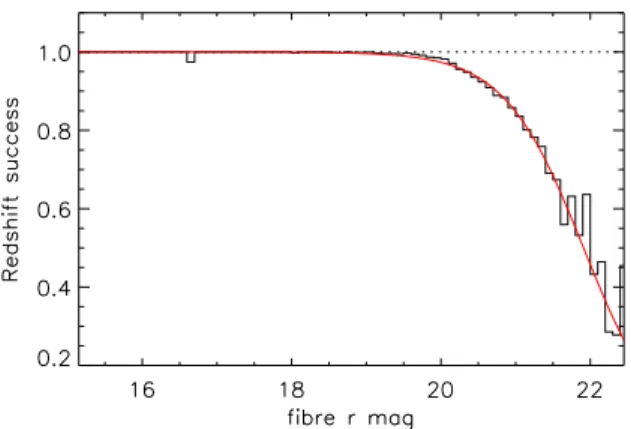
Redshift success rate is most likely to depend on the flux that goes down a 2dF fibre, that is a seeing-convolved 2-arcsec-diameter aperture. The closest quantity available in the SDSS database is

Figure 3.GAMA redshift success rate as a function of fibrer-band magni-tude plotted as a black histogram, with the horizontal dotted line indicating 100 per cent success. The red curve shows the best-fit sigmoid function.

fiberMag_r, hereinafterrfibre, corresponding to the flux

con-tained within a 3-arcsec-diameter aperture centred on the galaxy. We therefore determine histograms ofrfibre(uncorrected for

Galac-tic extinction) for all objects with high-quality redshifts (nQ >2) and for all objects with spectra. The ratio of these two histograms then gives redshift success as a function ofrfibre, and is shown in

Fig. 3. Note that some spectra observed in poor conditions have been re-observed at a later date in order to obtain this high success rate.

We see that redshift success rate is essentially 100 per cent for

rfibre<19.5, declines gently to around 98 per cent byrfibre= 20

and then declines steeply at fainter magnitudes. We have fitted a sigmoid functionf = 1/(1 +ea(rfibre−b)_{)to the binned success}

rate. Sigmoid functions have previously been used to model survey completeness, e.g. by Ellis & Bland-Hawthorn (2007). Our best-fit sigmoid function has parametersa= 1.89mag−1,b= 21.91mag, shown by the red line in Fig. 3, and we use this fit in determining redshift success rate.

2.3.4 Galaxy weights

Each galaxy is given a weight which is equal to the reciprocal of the product of the imaging completeness, target completeness and red-shift success rate. Imaging completenessCimis determined from

the galaxy’s apparentr-band half-light surface brightness,µ50,rby

linear interpolation of the curve in Fig.1. Target completenessCtarg

is determined separately in each band from the galaxy’s magnitude according to Fig. 2 and the spectroscopic success rateCspecis

de-termined from the sigmoid function fit described in section 2.3.3. The weightWiassigned to galaxyiis then

Wi= 1/(CimCtargCspec). (2)

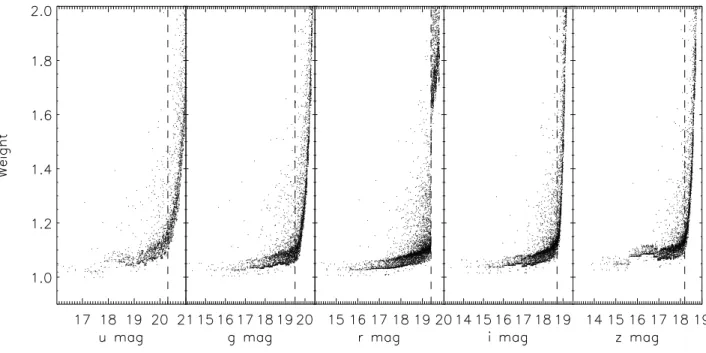
These weights, as a function of magnitude in each band, are shown for a randomly selected 5 per cent of galaxies in Fig. 4. The ma-jority of galaxies brighter than our magnitude limits have weight

Wi<1.1, with a small fraction extending toWi'2.

2.4 Velocity corrections

The redshifting softwareRUNZ (Saunders, Cannon & Sutherland 2004) provides heliocentric redshifts. Before converting heliocen-tric redshifts to any other velocity reference frame, we first

elimi-nate likely stars from our sample by rejecting objects with a helio-centric redshiftzhelio <0.002(cz <600km/s). This lower

red-shift cut is conservatively chosen, as the2nd Catalogue of Radial Velocities with Astrometric Data(Kharchenko et al. 2007) includes only one star with radial velocityRV >500km/s, and the vast ma-jority of Galactic stars haveRV <200km/s. Furthermore, Fig. 7 of Driver et al. (2011) shows that the redshift-error distribution for GAMA is essentially zero bycz= 600km/s.

Having eliminated 2111 likely stars from our sample, he-liocentric redshifts are converted to the CMB rest frame zCMB

according to the dipole of Lineweaver et al. (1996). For nearby galaxies (zCMB <0.03), we apply the multiattractor flow model

of Tonry et al. (2000). Note there are triple-valued solutions of

zCMB→zTonryover a small range in G12 (near the Virgo cluster),

here the average distance is used. The solution is tapered tozCMB

fromzCMB= 0.02tozCMB= 0.03(see Baldry et al. 2011 for

de-tails). We will see later that the Tonry et al. flow correction affects only the very faintest end of the LF.

2.5 K-corrections

When estimating intrinsic galaxy luminosities, it is necessary to correct for the fact that a fixed observed passband corresponds to a different range of wavelengths in the rest frames of galaxies at different redshifts, the so-calledK-correction (Humason, May-all & Sandage 1956). TheK-correction depends on the passband used, the redshift of the galaxy and its spectral energy distribu-tion (SED). Here we useKCORRECT V4 2 (Blanton et al. 2003a; Blanton & Roweis 2007) in order to estimate and apply these cor-rections. Briefly, this code estimates an SED for each galaxy by finding the non-negative, linear combination of five template spec-tra that gives the best fit to the five SDSS model magnitudes of that galaxy.KCORRECTcan then calculate theK-correction in any given passband at any redshift. Before callingKCORRECTitself, we useK SDSSFIXto convert SDSS asinh magnitudes to the AB sys-tem and to add in quadrature to the randomugrizmag errors given in the SDSS database typical systematic errors of (0.05, 0.02, 0.02, 0.02, 0.03) mag respectively.

We determine K-corrections in a passband blueshifted by

z0= 0.1. These magnitudes are indicated with a superscript prefix

of 0.1, e.g.0.1_M

r. This choice of rest frame allows direct

compar-ison with most previously published LFs based on SDSS data. Our LF estimators requireK-corrections to be calculated for each galaxy at many different redshifts in order to work out visibil-ity limits. To make this calculation more efficient, we fit a fourth-order polynomialPk(z) =P4_i=0ai(z−z0)i, withz0= 0.1, to the K(z)distribution for each galaxy and use this polynomial fit to de-termineK-corrections as a function of redshift. Using a polynomial of this order, the rms difference between theKCORRECTprediction and the polynomial fit is 0.01 mag or less in all five bands. Calcu-latedK-corrections and their polynomial fits are shown for the first four galaxies in our sample, along with the medianK-corrections and the 5 and 95 percentile ranges for the full sample, in Fig. 5.

Strictly, one should use heliocentric redshift when calculat-ingK-corrections, since they depend on theobservedpassband. However, for consistency with finding the minimum and maximum redshifts at which a galaxy would still be visible when using the

1/Vmax LF estimator, we use the flow-corrected redshift as

Figure 4.Completeness-correction weights as a function of magnitude for a random 5 per cent subset of GAMA galaxies. The vertical dashed lines show the magnitude limits applied in the LF analysis of each band.

2.6 Colour sub-samples

As well as analysing flux-limited samples of galaxies in theugriz

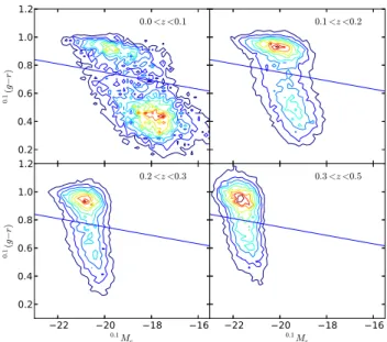
bands (hereafter the combined sample), we separate the galaxies into blue and red sub-samples. Following Zehavi et al. (2011), we use a colour cut based onK-corrected(g−r)model colour and absoluter-band magnitude that is insensitive to redshift:

0.1

(g−r)model= 0.15−0.030.1Mr, (3)

We have adjusted the zero-point of 0.21 mag in Zehavi et al. (2011) to 0.15 mag in order to better follow the ‘green valley’ and to get more equal-sized samples of blue and red galaxies. This colour cut works well at all redshifts (Fig. 6), although we see that the colour bimodality becomes far less obvious beyond redshiftz = 0.2due to the lack of low-luminosity, blue galaxies at these high redshifts. Although colour bimodality is more pronounced in(u−r)

colour, e.g. Strateva et al. (2001), Baldry et al. (2004),u-band pho-tometry, even after forming a ‘pseudo-Petrosian’ magnitude (equa-tion 1) is rather noisy, and so we prefer to base our colour cuts on the more robust(g−r)colour. This colour cut (in the original form of Zehavi et al.) has also been used to investigate the angular clustering of galaxies by Christodoulou et al. (2011). One should also note that colour is not a proxy for galaxy morphology: many red galaxies are in fact dust-obscured disc galaxies (Driver et al. in prep.).

2.7 Outlier inspection

We measure the LF over a very wide range of luminosities,−23to −11mag in therband. Galaxies at the extremes of this luminos-ity range are very rare in a flux-limited survey, due either to their intrinsic low number density at high luminosity or small detection volume at low luminosity, and thus it is likely that a significant fraction of these putative extreme objects are in fact artifacts due to incorrectly assigned redshifts or magnitudes. The first author has

Table 1.Classification of extreme high- and low-luminosity objects.

POST CLASS 0.1Mu<−20mag 0.1Mr>−15mag

1 OK 4,743 299

2 QSO 18 0

3 Major shred 68 62

4 Minor shred 0 7

5 Problem deblend 151 16

6 Bad sky background 246 14

therefore inspected image cutouts showing SDSS image detections of 5,226 very luminous GAMA targets with0.1Mu < −20mag

and 398 very faint targets with0.0Mr>−15mag. We choose the

uband to select luminous outliers since theu-band LF shows the largest bright-end excess.

Table 1 shows how the inspected images were classified. The classification codes, which we callPOST CLASSin order to distin-guish them from the pre-target-selectionVIS CLASShave the fol-lowing meanings.

(1) OK — nothing from the image would lead one to expect poor photometry for that object.

(2) The object looks like a QSO, i.e. blue and point-like. This classification is ignored in the analysis (treated as OK) due to the difficulty of distinguishing QSOs and compact blue galaxies from the imaging data alone.

(3) The central part of a galaxy which has been shredded into multiple detections. It is likely that the luminosity is somewhat un-derestimated in these cases.

(4) The target is a minor part of a shredded galaxy. Luminosity is likely to be greatly underestimated.

(5) The galaxy is very close to a second object which either has not been deblended, or is likely to significantly affect the estimated luminosity in either direction.

Figure 5.Top four panels:K-corrections as a function of redshift (red, blue, green, magenta and yellow respectively forugriz) for the first four galaxies in our sample. Black dashed lines show fourth-order polynomial fits to each band. Bottom panel: medianK-corrections (coloured continuous lines) and 5 and 95 percentile ranges (dotted lines) for the entire GAMA sample. Black dashed lines show fourth-order polynomial fits to the medians.

0.2 0.4 0.6 0.8 1.0 1.2

0

.

1(g

−

r

)

0.0<z <0.1 0.1<z <0.2

0.2 0.4 0.6 0.8 1.0 1.2

0

.

1(g

−

r

)

22 20 18 16

0.1_M r

0.2<z <0.3

22 20 18 16

0.1_M r

0.3<z <0.5

Figure 6.0.1_{(g−r)colour versus}0.1_M

rr-band absolute magnitude

tour plots for GAMA galaxies in four redshift ranges as labelled. Ten con-tours, spaced linearly in density, are colour-coded from black to red in or-der of increasing density. The straight line shows the magnitude-dependent colour cut separating blue and red galaxies given by equation (3).

(6) Photometry is likely severely compromised by rapidly vary-ing sky background due typically to the presence of a nearby satu-rated star.

Examples of objects with these classifications are shown in Fig. 7. In practice, there is some ambiguity in assigning a galaxy with clas-sification 4 or 5, but as far as the LF analysis is concerned, it makes no difference.

These inspections were based on version 10 of the GAMA tiling catalogue, excluding objects withVIS CLASS= 2–4. The ma-jor and minor shreds in Table 1 have also been inspected by IKB. In the case of major shreds, we have summed the flux from the compo-nents of the shredded galaxy to derive a ‘deblend-fixed’ magnitude. In total, 281 GAMA-I galaxies have had their magnitudes fixed in this manner.

In the case of six minor shreds which both JL and IKB agreed on, the value ofVIS CLASS has been set equal to 3 in the latest version (v16) of the tiling catalogue.

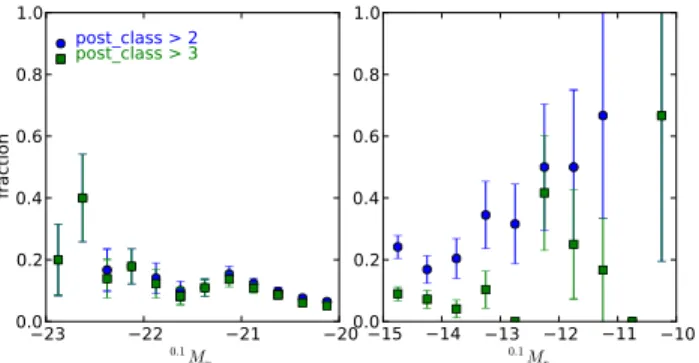
The fractions of galaxies withPOST CLASSof 3 or 4 or higher as a function ofMuandMrare shown in Fig. 8. We see in the left

panel that by magnitudes ofMu=−20, less than 10 per cent of

objects have suspect photometry. Once we allow for fixing of over-deblended galaxies, a similar fraction of objects withMr ' −15

have suspect photometry (right panel).

For our analysis, we have chosen to exclude any galaxies with

POST CLASSof 4 or higher, i.e. we include major shreds with fixed fluxes but exclude minor shreds, problem deblends and bad sky objects. Fig. 9 shows the ratio of the r and u band LFs using

POST CLASS< 4galaxies to that determined using all galaxies. We see that excluding objects with suspect photometry has a rela-tively minor effect on the determined LF: the very bright end and some faint-end bins are systematically lower by up to 50 per cent; these changes are comparable to the size of the error bars.

1

2

3

4

5

6

Figure 7.Examples of objects classified from 1 to 6. The GAMA targets are at the centre of each image, which are 40 arcsec on each side. The colour table has been inverted, so that red objects appear blue and vice-versa, in order to obtain a light background. Circles denote SDSS image detections: multiple circles on a single object (example classifications 3 and 4) suggest that it has been over-deblended.POST CLASSclassifications are shown in the top-left corner of each image, their meaning is given in Table 1.

23 22 21 20

0.1_M u

0.0 0.2 0.4 0.6 0.8 1.0

fraction

post_class > 2 post_class > 3

15 14 13 12 11 10

0.1_M r

0.0 0.2 0.4 0.6 0.8 1.0

Figure 8.Fraction of objects withPOST CLASS>2(blue circles) and>3

(green squares) as a function of0.1_M

u(left panel) and0.1Mr(right panel).

Error bars show Poisson errors on the counts.

24 22 20 18 16 14 12 10

0.1_M r−5logh

0.0 0.5 1.0 1.5 2.0

φ

(

M

)

/φ0

(

M

)

22 20 18 16 14 12 10

0.1_M u−5logh

0.0 0.5 1.0 1.5 2.0

φ

(

M

)

/φ0

(

M

)

Figure 9.Ratio of LFs determined usingPOST CLASS≤3objects to that using all objects inrband (top) anduband (bottom). Symbols show ratio of SWML estimates and their uncertainties, the continuous lines shows the ratio of parametric fits to the two samples.

luminosity. Our four faintestr-band luminosity galaxies are also in the Brough et al. sample.

3 ESTIMATING THE LUMINOSITY FUNCTION AND ITS EVOLUTION

3.1 Parameterizing the evolution

In order to parametrize the evolution of the galaxy LF, we follow Lin et al. (1999) in assuming a Schechter (1976) function in which the characteristic magnitudeM∗and galaxy densityφ∗are allowed to vary with redshift, but where the faint-end slopeαis assumed to be non-evolving.4

Specifically, in magnitudes, the Schechter function is given by

φ(M) = 0.4 ln 10φ∗(100.4(M∗−M))1+αexp(−100.4(M∗−M)),

(4) where the Schechter parametersα,M∗andφ∗vary with redshift as:

α(z) =α(z0),

M∗(z) =M∗(z0)−Q(z−z0), (5)

φ∗(z) =φ∗(0)100.4P z.

Here the fiducial redshiftz0is the same redshift to which

magni-tudes areK-corrected, in our casez0= 0.1. The Schechter

param-etersα,M∗(z0)andφ∗(0)and evolution parametersQandPare

determined via the maximum-likelihood methods described by Lin et al. (1999).

4 _{Evolution in the LF faint-end slopeαwith redshift is still rather poorly}

constrained. Ellis et al. (1996) claim thatαsteepens with redshift, due to an increase in the number of faint, star-forming galaxies atz'0.5. Ilbert et al. (2005) also measure a possible steepening ofαwith redshift. In contrast, Liu et al. (2008) find thatαgets shallower at higher redshifts. Our assump-tion of fixedαis largely based on practical necessity, sinceαcan only be reliably measured at redshiftsz <_∼0.2from the GAMA data.

First, the shape parametersα,M∗(z0)and luminosity evolu-tion parameterQare fit simultaneously and independently of the other parameters by maximising the log likelihood

lnL=

Ngal

X

i=1

Wilnpi. (6)

Here,Wiis the incompleteness correction weighting (equation 2)

and the probability of galaxyihaving absolute magnitudeMigiven

its redshiftziis

pi≡p(Mi|zi) =φ(Mi)

,

Z min[Mmax(zi),M2]

max[Mmin(zi),M1]

φ(M)dM ,

(7) whereM1,M2 are the absolute magnitude limits of the sample, Mmin(zi), Mmax(zi) are the minimum and maximum absolute

magnitudes visible at redshiftzi, andφ(M)is the differential LF

given by (4).

The density evolution parameterP and normalizationφ∗(0)

cancel in the ratio in (7) and so must be determined separately. Lin et al. show that the parameterPmay be determined by maximising the second likelihood

lnL0=

N_gal

X

i=1

Wilnp0i, (8)

where

p0i≡p[zi|Mi(0), Q]

= 100.4P zi

,

Z min[zmax[Mi(0),z2]

max[zmin[Mi(0)],z1]

100.4P zdV

dzdz , (9)

wherez1,z2are the redshift limits of the sample,zmin,zmaxare

the redshift limits over which galaxy imay be observed, given the survey’s apparent magnitude limits and its absolute magnitude evolution-corrected to redshift zero,Mi(0) =Mi(zi) +Qzi. Note

that the value ofPis independent of the fiducial redshiftz0.

Finally, we fit for the overall normalisationφ∗(0). We depart slightly from the prescription of Lin et al. (1999) here. In place of their equation 14, we use a minimum variance estimate of the space densityn¯of galaxies:

¯ n=

Ngal

X

i=1

WiU(zi)

100.4P zi

Z zmax

zmin

dV

dzS(z)U(z)dz , (10)

where S(z) is the galaxy selection function, U(z) a redshift weighting function chosen to give minimum variance anddV /dzis the volume element at redshiftz. The selection function for galax-ies with luminositgalax-iesL1toL2is

S(z) =

Z min(Lmax(z),L2)

max(Lmin(z),L1)

φ(L, z)dL

Z L2

L1

φ(L, z)dL . (11)

Note that the integration limits in the numerator depend on the as-sumedK-correction. In this case, we use the medianK-correction of the galaxies in the sample under consideration: see Fig.5 for me-dianK-corrections for the full sample as a function of redshift. Our results change by much less than the estimated 1-sigma errors (see Section 3.5) if we use mean instead of medianK-corrections.

We adopt the redshift weighting function

U(z) = 1

1 + 4π(¯n/W¯)J3(rc)S(z)

, J3(rc) =

Z rc

0

r2ξ(r)dr,

(12) whereξ(r)is the two point galaxy correlation function andW¯ is

the mean incompleteness weighting. ProvidedJ3(rc) converges

on a scale rc much smaller than the depth of the survey, then

this redshift weighting scheme (equation 12) minimizes the vari-ance in the estimate ofn¯(Davis & Huchra 1982). Larger values of J3 weight galaxies at high redshift more highly; we assume 4πJ3= 30,000h−3Mpc3. This value comes from integrating the

flux-limited two-point galaxy correlation function of Zehavi et al. (2005),ξ(r) = (r/5.59)−1.84

, torc= 60h−1Mpc; at larger

sepa-rations the value ofJ3becomes uncertain. However, the results are

not too sensitive to the value ofJ3, the estimated densities changing

by less than 8 per cent ifJ3is halved. This possible systematic

er-ror is generally comparable to or less than the statistical uncertainty inφ∗(5– 25 per cent).

We check our minimum variance normalisation by comparing, in Tables 3, 4 and 5, the observed number of galaxies in each sam-ple (within the specified apparent magnitude, absolute magnitude and redshift limits) with the prediction

Npred= 1 ¯ W

Zzmax

zmin

Z Lmax(z)

Lmin(z)

φ(L, z)dV

dzdz. (13)

3.2 Luminosity density

Given our assumed evolutionary model, the predicted LD is given by

ρLfit=ρL(0)100.4(P+Q)z, (14)

(Lin et al. 1999 equation 11), where

ρL(0) =

Z

Lφ(L, z= 0)dL=φ∗(0)L∗(0)Γ(α+ 2), (15)

andΓ(x)is the standard Gamma function. In making this predic-tion, we are integrating over all possible luminosities, and hence extrapolating our Schechter function fits. This extrapolation intro-duces no more than 1 per cent in additional LD beyond that con-tained within our luminosity limits. We obtain luminosities in solar units using the following absolute magnitudes for the Sun in SDSS bandpasses:0.1M_u,g,r,i,z−5 lgh= 6.80,5.45,4.76,4.58,4.51 mag (Blanton et al. 2003b).

We also directly determine LD as a function of redshift by summing the weighted luminosities of galaxies in a series of red-shift bins:

ρLj=

1 Vj

X

i∈j

WiLi

SL(zi)

. (16)

(Lin et al. equation 16). HereVjis the volume of redshift binj, the

sum is over each galaxyiin binjand the factor

SL(z) =

Z min(Lmax(z),L2)

max(Lmin(z),L1)

Lφ(L, z)dL

Z ∞

0

Lφ(L, z)dL ,

(17) (Lin et al. equation 17) extrapolates for the luminosity of galaxies lying outside the accessible survey flux limits.

3.3 Binned LF estimates

In order to assess how well the model (equation 5) parametrizes LF evolution, we also make non-parametric, binned, estimates of the LF in independent redshift ranges using the1/Vmax(Schmidt

Figure 10.Illustration of estimatingφ(M, z)in bins of absolute magnitude M and redshiftzrepresented by dotted lines for a fictitious survey with apparent magnitude limitsmbright = 14.5andmfaint = 18. Galaxies

(represented by points) are of course only found between these flux limits, corresponding to the lower and upper curved lines respectively. Now con-sider the highlighted bin, centred onM =−19.5and with redshift limits zlo= 0.10,zhi = 0.15. At the lower redshift limit, the absolute

magni-tude corresponding tomfaintisM ' −19.6. Since this is mid-bin, the

LF estimated for this bin would be underestimated, and therefore the bin should be excluded. Thus for the redshift slice0.10 < z < 0.15, only magnitude bins brightward ofM=−20should be used. (The fact that the magnitude bin centred onM=−20.5is incomplete at redshiftsz > zlo

will be compensated for by1/Vmaxweighting.) A similar incompleteness

may arise for bins at low redshift and high luminosity. For the redshift slice

0.00< z <0.05, only magnitude binsfainterthanM=−21should be

used.

bins fromM =−25toM =−10with∆M = 0.25and a series of redshift slices.

When estimating the LF over restricted redshift ranges, one has to be careful to only include magnitude bins that are fully sam-pled, since otherwise the LF will be underestimated in incompletely sampled bins, see Fig. 10. We therefore set the following magni-tude limits for each redshift slice so that only complete bins are included:

Mfaint< mfaint−DM(zlo)−K(zlo),

Mbright> mbright−DM(zhi)−K(zhi). (18)

Here,mfaintandmbrightare the flux limits of the survey,DM(z)

is the distance modulus,K(z)is theK-correction for a galaxy with the median SED of those in the survey,zloandzhiare the limits of

the redshift slice under consideration, andMfaintandMbrightare

the absolute magnitude limits of each bin. A bin should only be included if it satisfies both equations (18).

Again following Lin et al. (1999), we incorporate the galaxy incompleteness weights into the SWML maximum likelihood esti-mator by multiplying each galaxy’s log-probability by its weight before summing to form a log-likelihood (equation 6). In the

1/Vmaxestimate, we form a sum of the weight of each galaxy

di-vided by the volume within which it is observable. We normalize the SWML estimatesφSWMLin each redshift slice to the1/Vmax

estimatesφVmaxby imposing the constraint

Nbin

X

k=1

φSWMLkV(Mk) =

Nbin

X

k=1

φVmaxkV(Mk), (19)

where V(Mk) is the volume (within the redshift limits of each

slice) over which a galaxy of absolute magnitudeMk, being the

mean galaxy absolute magnitude in bink, is visible. The predicted number of galaxies

NSWML= 1 ¯ W

Nbin

X

k=1

φkV(Mk)∆M (20)

may also be compared with the observed number of galaxies within each redshift range.

We can use our SWML LF estimates to assess the quality of the parametric fits using a likelihood ratio test (Efstathiou, Ellis & Peterson 1988). In this test, we compare the log-likelihoodslnL1

andlnL2given by equation (6) for the SWML and parametric

es-timates respectively. The log likelihood ratio−2 ln(L1/L2)is

ex-pected to follow aχ2 distribution withν = Np−4degrees of

freedom. HereNpis the number of bins in the stepwise estimate

and we subtract 1 degree of freedom for each of the fitted shape parametersα,M∗(0)andQand for the arbitrary normalisation.

To allow for the finite bin sizes and redshift ranges of the SWML estimates, we calculate binned estimates of the parametric fits. These are given by (Lin et al. 1999)

φz1−z2

k =

RMk+∆M/2

Mk−∆M/2

Rmin[zmax(M),z2]

max[zmin(M),z1] φ 2

(M, z)dV_dzdz dM

RMk+∆M/2

Mk−∆M/2

Rmin[zmax(M),z2]

max[zmin(M),z1]φ(M, z)

dV dzdz dM

.

(21) Here, the parametric LF φ(M, z) is weighted by the number of galaxies at each magnitude and redshift, given by the factor

φ(M, z)dV_dz . These binned versions of the parametric fits are also used when plotting the LFs. For absolute magnitudes in all plots, we use the weighted mean magnitude of the galaxies in each bin, rather than using the magnitude of the bin centre. This helps to overcome the bias due to the finite width of magnitude bins.

3.4 LF faint end

It is now widely recognised that a Schechter function provides a poor fit to galaxy LFs when measured over a wide range of magni-tudes (e.g. Blanton et al. 2005b). In order to parametrize the faint end, we separately analyse a low redshift (z <0.1) subset of the data and fit (non-evolving) double power-law Schechter functions.

We use the parameterization of Loveday (1997), namely

φ(L) =φ∗

L L∗

α

exp

−L

L∗

"

1 +

L Lt

β#

. (22)

In this formulation, the standard Schechter function is multiplied by the factor[1 + (L/Lt)β], whereLt< L∗is a transition luminosity

between two power-laws of slopeα(LLt) andα+β(LLt).

It is fitted to unbinned data using an extension to the method of Sandage, Tammann & Yahil (1979). With this four-parameter fit (the normalisationφ∗is fitted separately), one has to be careful to choose sensible starting values in order for the downhill simplex algorithm(scipy.optimize.fmin) not to get stuck in local minima of−lnL. (We also found that it helped to call the mini-mizer several times, using ‘best-fitting’ parameters from one func-tion call as starting parameters for the next;−lnLwas found to converge with 2–4 calls of the minimizer.)

Note that the double power-law Schechter function may equiv-alently be written as the sum of two Schechter functions, e.g. Blan-ton et al. (2005b); Baldry, Glazebrook, Driver (2008), a fact which comes in useful when integrating the LF.

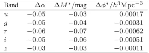
Table 2.Change in fitted Schechter parameters for combined samples when applying imaging completeness correction.

Band ∆α ∆M∗_{/mag ∆φ}∗_/h3_Mpc−3

u −0.05 −0.03 0.00017

g −0.05 −0.04 −0.00031

r −0.06 −0.07 −0.00062

i −0.05 −0.06 −0.00051

z −0.03 −0.03 −0.00011

When fitting a double power-law Schechter function, the like-lihood ratio test hasν = Np−5 degrees of freedom (cf.

sec-tion 3.3).

3.5 Error estimates

Schechter and evolution parameter estimates are strongly corre-lated, and so in Section 4 we present 95 per cent likelihood contour plots of shape parameters α, M∗, β,Mt and evolution

parame-ters Q, P. For uncertainties in tabulated measurements, we esti-mate errors using the jackknife technique, as follows. We divide the GAMA survey area into nine regions, each4×4deg2. We then calculate the LF and LD using the methods discussed above, omitting each region in turn. For any parameterx, we may then determine its variance using

Var(x) =N−1 N

N

X

i=1

(xi−¯x)2, (23)

whereN = 9is the number of jackknife regions andx¯is the mean of the parametersximeasured while excluding regioni. The

jack-knife method has the advantage of providing error estimates which include both uncertainties in the fitted parameters as well as sample variance.

The sample variance in galaxy densitynmay also be deter-mined using:

δn

n 2

=4πJ3

V , (24)

(Davis & Huchra 1982; Efstathiou, Ellis & Peterson 1988), where

J3is defined in (12) andV is the volume of each sample between

redshift limits.

For errors on binned LFs, we use Poisson errors for1/Vmax

estimates and an inversion of the information matrix for SWML estimates (Efstathiou, Ellis & Peterson 1988).

4 RESULTS

Before presenting our main results, we first check the effects of correcting for imaging completeness and the choice of flow model in converting redshifts to distances.

4.1 Imaging completeness correction

In Fig. 11, we comparer-band LFs calculated for the combined sample, with distances calculated using the Tonry et al. (2000) mul-tiattractor flow model, with and without the correction for imag-ing completeness described in Section 2.3.1. As expected, we see that applying imaging completeness corrections boosts the LF faint end, while barely changing the bright end. The changes in fitted Schechter parameters due to imaging completeness corrections are

22 20 18 16 14 12 10

0.1_M r−5logh

10-5

10-4

10-3

10-2

10-1

100

φ

(

M

)

h

3 M

pc

−

3

Figure 11.LF estimates in therband for low-redshift galaxies (z <0.1) with (solid symbols and line) and without (open symbols, dashed line) ap-plying a correction for imaging completeness. Symbols show SWML esti-mates, lines show best-fitting Schechter functions.

22 20 18 16 14 12 10

0.1_M r−5logh

10-5

10-4

10-3

10-2

10-1

100

φ

(

M

)

h

3 M

pc

−

3

Figure 12.LF estimates in therband for low-redshift galaxies (z <0.1) using the CMB reference frame (open circles) and the Tonry et al. (2000) multiattractor flow model (filled circles) using the SWML estimator. Solid and dashed lines show the best-fit Schechter functions which are indistin-guishable.

tabulated in Table 2. Future plots and tabulated parameters will in-clude imaging completeness corrections; approximate uncorrected Schechter parameters may be obtained by subtracting the appropri-ate quantities listed in Table 2.

4.2 Effects of velocity flow model

Luminosities of galaxies at the extreme faint end of the LF, being very close by, will be sensitive to peculiar velocities. In Fig. 12, we comparer-band LFs calculated using the CMB reference frame (Lineweaver et al. 1996) and the Tonry et al. (2000) multiattractor flow model for galaxies at low redshift (z <0.1). We see that the CMB-frame and flow model LFs only begin to differ at the extreme faint end,Mr−5 logh >_{∼ −}15mag, and even at these faint

10

-7

10

-6

10

-5

10

-4

10

-3

10

-2

10

-1

_u

10

-7

10

-6

10

-5

10

-4

10

-3

10

-2

10

-1

_g

10

-7

10

-6

10

-5

10

-4

10

-3

10

-2

10

-1

φ

(

M

)

/

h

3

M

pc

−

3

r

10

-7

10

-6

10

-5

10

-4

10

-3

10

-2

10

-1

_i

10

-7

10

-6

10

-5

10

-4

10

-3

10

-2

10

-1

24

22

20

18

16

14

12

10

0

.

1

_M

−

5log

h

z

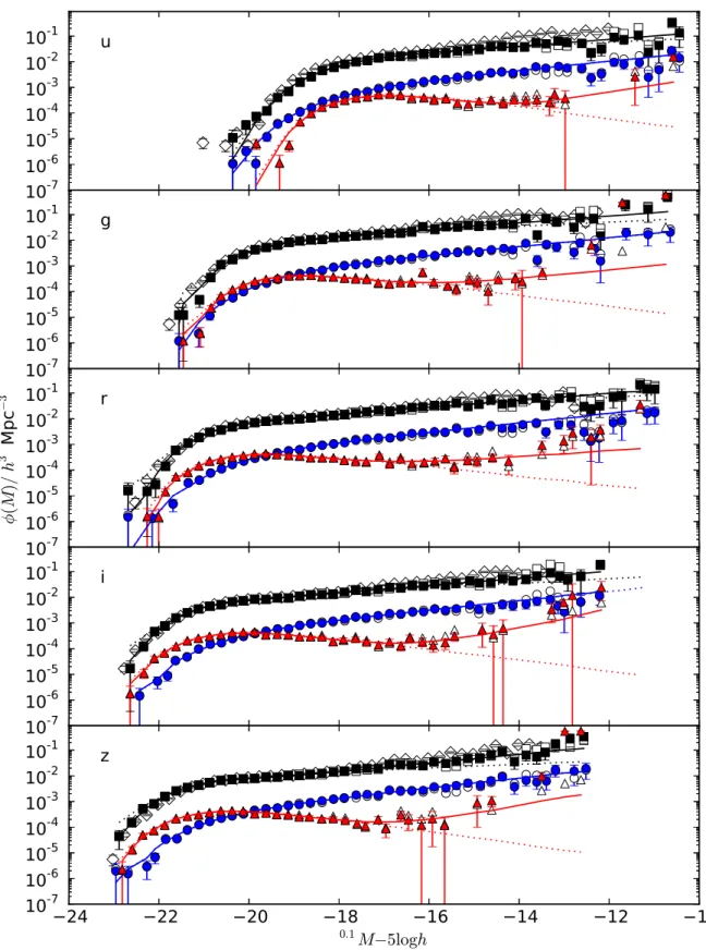
Figure 13.ugrizLFs at low redshift (z <0.1). Black squares show SWML estimates for combined red and blue samples, blue circles and red triangles show SWML LFs for the blue and red samples respectively. Open symbols of the same shapes show the corresponding1/Vmaxestimates — these are hidden

beneath the SWML estimates for all but the very faintest galaxies. Continuous lines show the best-fit non-evolving double power-law Schechter function fits, dotted lines show standard Schechter function fits. LFs for the blue and red samples have been scaled by a factor of 0.1 to aid legibility. Open diamonds show the ‘corrected’ LF (without colour selection) from Blanton et al. (2005b).

In particular, the recovered Schechter parameters are indistinguish-able between the two velocity frames. Subsequent analysis will use the Tonry et al. flow model to determine luminosities.

4.3 Luminosity function faint end

Having looked at the effects of incompleteness and flow correc-tions, we now study in detail the faint end of the LF for low red-shift (z <0.1) galaxies. Fig. 13 shows the LFs for our three (com-bined, blue and red) samples in theugrizbands. Also shown are LFs corrected for surface brightness incompleteness by Blanton et al. (2005b) from the New York University Value-Added Galaxy Catalog (NYU-VAGC) low-redshift sample (Blanton et al. 2005a). Since these Blanton et al. LFs were calculated using restframeK -corrections, we apply an offset of2.5 lg(1 +z0)to their absolute magnitudes in order to convert to ourz0 = 0.1band-shiftedK

-corrections. Our faint-end LFs are systematically lower than those of Blanton et al., particularly in theu band. The difference can largely be explained by the different flow models used by Blanton et al. and in the present analysis. Re-analysing the Blanton et al. data using the Tonry et al. flow model results in much better agree-ment (Baldry et al. 2011) — the extra 1.7 mag depth of the GAMA versus the SDSS main galaxy sample means that uncertainties due to the flow model affect the measured LF only at a correspondingly fainter magnitude.

Table 3 shows the number of galaxies and absolute magni-tude limits for each sample, along with the parameters of stan-dard Schechter function fits and luminosity densities. Only for blue galaxies in theu,iandzbands does a standard Schechter function provide a statistically acceptable fit to the data at the 2 per cent level or better. For red galaxies, we observe a decline in number density faintwards of the characteristic magnitudeM∗with a subsequent increase in faint-end slope atMt ∼M∗+ 3. For the red galaxies,

and the combined sample, a double-power-law Schechter function (22) is required to fit the shape of the observed LFs. These findings are in apparent agreement with the predictions of halo occupation distribution models, e.g. Brown et al. (2008), in which luminous red galaxies are central galaxies, but fainter red galaxies are in-creasingly more likely to be satellites in relatively massive halos. An alternative perspective is provided by Peng et al. (2010), who explain the change in faint-end slope of red galaxies via a simple picture for the quenching of star formation by the distinct processes of ‘mass quenching’ and ‘environment quenching’. Our results pro-vide the most precise demonstration of the changing faint-end slope of red galaxies to date.

However, the observed upturn needs to be interpreted with caution, since, from a quick visual inspection, the 164 faint (0.1Mr−5 lgh >−16mag), red galaxies that comprise the

up-turn include a significant fraction ('50per cent) of galaxies that appear to be disc like, as well as a number of artifacts. It thus seems likely that dust-reddened disc systems, as well as dwarf galaxies with intrinsically red stellar populations, contribute to the faint-end upturn in the red galaxy LF. Future work will investigate the LF dependence on morphology and dust reddening, utilising GAMA’s multi-wavelength coverage.

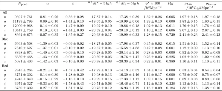
Double-power-law Schechter function fits are given in Ta-ble 4. Likelihood ratio tests show that the douTa-ble-power-law Schechter function provides significantly better fits than the stan-dard Schechter function for the combined and red galaxy samples, at least for the redder bands. For the blue galaxies, however, the double-power-law Schechter function fits are actually worse than

1.0 0.5_α 0.0 0.5 21 20 19 18 17 0 . 1M ∗− 5l g h u g r i z

1.0 0.5_α 0.0 0.5 2.5 2.0 1.5 1.0 0.5 0.0 β u

g r i z

1.0 0.5 0.0 0.5

α 21 20 19 18 17 16 15 14 0 . 1M t − 5l g h u g r i z

21 20 19 18 17

0.1_M∗_−5lgh

2.5 2.0 1.5 1.0 0.5 0.0 β u g r i z

21 20 19 18 17

0.1_M∗_−5lgh

21 20 19 18 17 16 15 14 0 . 1M t − 5l g h u g r i z

2.5 2.0 1.5 1.0 0.5 0.0

β 21 20 19 18 17 16 15 14 0 . 1M t − 5l g h u g r i z

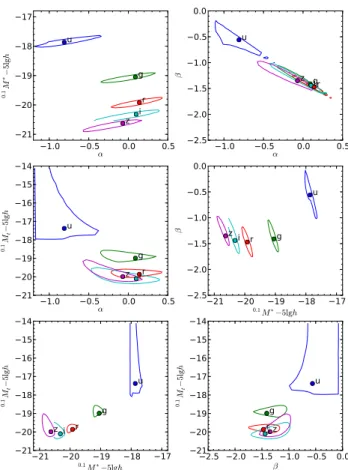
Figure 14.2-σlikelihood contours for various parameter pairs in double power-law Schechter function fits to the combined sample forugrizbands as labelled.

the standard Schechter function fits when taking into account the two additional degrees of freedom.

The quoted errors need to be treated with caution due to strong correlations between the parameters, particularly in the case of the five-parameter, double power-law Schechter function fits. Fig. 14 shows 2σ likelihood contours for each pair of parameters from

α, M∗, β and Mt for the combined sample. We see that αand

β individually are very poorly constrained, with an uncertainty

∆α'∆β '0.5. However, the overall faint-end slopeα+βis very well constrained, with a consistent value in all five passbands

α+β=−1.37±0.05for the combined sample. For blue galaxies,

α+β=−1.50±0.03and for red galaxies,α+β=−1.6±0.3. Consistent faint-end slopes are found for the stellar mass function (Baldry et al. 2011) . Also from Fig. 14, we see that the charac-teristic magnitudeM∗ is positively correlated with slope αbut negatively correlated withβ. The transition magnitudeMtis only

weakly correlated with either slope parameterαorβ and almost completely uncorrelated with the characteristic magnitudeM∗.

Fig. 15 shows2σlikelihood contours for the red sample. We see that, while still uncertain, the slope parametersαandβare only weakly correlated. The characteristic magnitudeM∗is positively correlated withαbut almost completely uncorrelated withβ. The transition magnitudeMtis strongly anti-correlated withαand

vir-tually independent ofβ.

Table 3.Standard Schechter function fits for low-redshift galaxies. Samples are as given in the first column.0.1_M

1and0.1M2are the absolute magnitude

limits,Ngalthe number of galaxies in the sample andNpredthe predicted number of galaxies from integrating the LF (equation 13).α,0.1M∗andφ∗are

the usual Schechter parameters, andPfitgives the probability of the Schechter function describing the observed LF determined from the likelihood ratio test

described in the text. Luminosity densitiesρLfitandρLsumare calculated via equations (15) and (16) respectively. 0.1_M

1 0.1M2 Ngal Npred α 0.1M∗−5 lgh φ∗×100 Pfit ρLfit ρLsum

−5 lgh /h3_Mpc−3 _/108_L

hMpc−3

All

u −21.0 −10.0 9181 9402±766 −1.21±0.03 −18.02±0.04 1.96±0.15 0.001 1.95±0.18 1.95±0.18

g −22.0 −10.0 11158 11085±781 −1.20±0.01 −19.71±0.02 1.33±0.12 0.000 1.79±0.14 1.79±0.15

r −23.0 −10.0 12860 12789±956 −1.26±0.02 −20.73±0.03 0.90±0.07 0.000 1.75±0.15 1.75±0.15

i −23.0 −11.0 10438 10341±745 −1.22±0.01 −21.13±0.02 0.90±0.08 0.000 2.06±0.18 2.06±0.18

z −24.0 −12.0 8647 8535±658 −1.18±0.03 −21.41±0.05 0.90±0.06 0.000 2.39±0.22 2.38±0.22

Blue

u −21.0 −10.0 6278 6664±509 −1.44±0.02 −18.27±0.04 0.88±0.05 0.028 1.50±0.14 1.52±0.14

g −22.0 −10.0 7356 7611±537 −1.42±0.02 −19.58±0.05 0.71±0.03 0.002 1.12±0.10 1.12±0.10

r −23.0 −10.0 8579 8893±680 −1.45±0.02 −20.28±0.07 0.55±0.03 0.000 0.92±0.09 0.92±0.09

i −23.0 −11.0 6432 6641±465 −1.45±0.02 −20.68±0.06 0.50±0.03 0.381 1.02±0.09 1.02±0.09

z −24.0 −12.0 4888 5089±400 −1.48±0.03 −20.99±0.07 0.41±0.02 0.477 1.11±0.11 1.10±0.11

Red

u −21.0 −10.0 2903 2850±263 −0.40±0.08 −17.34±0.06 1.29±0.12 0.000 0.52±0.05 0.53±0.05

g −22.0 −10.0 3802 3758±307 −0.47±0.07 −19.31±0.06 1.06±0.11 0.000 0.75±0.07 0.75±0.07

r −23.0 −10.0 4281 4265±354 −0.53±0.04 −20.28±0.06 0.98±0.09 0.000 0.90±0.08 0.89±0.08

i −23.0 −11.0 4006 4014±332 −0.46±0.03 −20.63±0.05 1.04±0.09 0.000 1.13±0.11 1.11±0.11

z −24.0 −12.0 3759 3760±301 −0.40±0.05 −20.87±0.06 1.10±0.07 0.000 1.39±0.13 1.38±0.13

Table 4.Double power-law Schechter function fits for low-redshift galaxies. Values for0.1M1,0.1M2andNgalare the same for each sample as in Table 3.

Other columns have the same meaning as the previous Table and in addition we tabulate the values of the double power-law Schechter parametersβandMt.

Npred α β 0.1M∗−5 lgh 0.1Mt−5 lgh φ∗×100 Pfit ρLfit ρLsum

/h3Mpc−3 /108LhMpc−3

All

u 9397±761 −0.81±0.26 −0.56±0.28 −17.87±0.14 −17.38±0.39 1.32±0.26 0.005 1.97±0.18 1.97±0.18

g 11199±798 0.09±0.10 −1.41±0.10 −19.05±0.05 −18.99±0.06 1.28±0.10 0.000 1.83±0.15 1.83±0.15

r 12900±968 0.14±0.09 −1.47±0.09 −19.92±0.10 −19.86±0.18 1.02±0.13 0.011 1.76±0.15 1.76±0.15

i 10447±759 0.10±0.01 −1.44±0.03 −20.32±0.04 −20.10±0.12 1.10±0.12 0.606 2.07±0.18 2.07±0.18

z 8664±675 −0.07±0.35 −1.35±0.27 −20.63±0.17 −19.99±0.33 1.28±0.15 0.729 2.41±0.23 2.41±0.23

Blue

u 6663±508 −1.39±0.03 −0.09±0.02 −18.27±0.05 −17.98±0.37 0.45±0.02 0.015 1.51±0.14 1.52±0.14

g 7610±527 −1.37±0.01 −0.10±0.02 −19.57±0.04 −15.58±4.88 0.42±0.08 0.001 1.12±0.09 1.13±0.10

r 8898±674 −1.40±0.05 −0.09±0.10 −20.28±0.05 −20.14±2.16 0.28±0.03 0.000 0.92±0.09 0.92±0.09

i 6650±468 −1.43±0.06 −0.05±0.09 −20.69±0.05 −19.76±1.47 0.25±0.03 0.225 1.02±0.09 1.02±0.09

z 5081±403 −1.42±0.03 −0.10±0.00 −20.98±0.08 −20.30±0.34 0.22±0.01 0.389 1.10±0.11 1.10±0.11

Red

u 2845±264 −0.21±0.16 −1.57±0.42 −17.22±0.10 −14.13±0.52 1.34±0.14 0.000 0.53±0.04 0.54±0.04

g 3751±302 −0.14±0.30 −1.28±0.29 −19.08±0.13 −16.39±1.46 1.14±0.17 0.000 0.75±0.07 0.75±0.07

r 4245±349 −0.15±0.29 −1.16±0.10 −19.99±0.15 −17.33±1.17 1.09±0.15 0.001 0.89±0.08 0.89±0.08

i 3974±327 −0.33±0.10 −1.58±0.43 −20.51±0.08 −16.46±0.71 1.12±0.10 0.228 1.13±0.14 1.13±0.14

z 3730±302 −0.27±0.20 −1.51±0.51 −20.75±0.12 −16.93±1.19 1.16±0.09 0.184 1.38±0.16 1.38±0.16

the contour plots contain no useful information, and hence are not shown.

In summary, in analysing the faint end of the LFs, we have found that:

(i) While a standard Schechter function provides an acceptable fit to the blue galaxy LF in all bands, the red galaxy LF exhibits a decline just faintwards ofM∗followed by a pronounced upturn at magnitudeMt 'M∗+ 3. Such an LF is well-fitted by a

double-power-law Schechter function.

(ii) We caution that the faint end of the red galaxy LF is possibly dominated by dust-reddened systems, rather than by galaxies with intrinsically red stellar populations.

(iii) Neither standard nor double-power-law Schechter function faint-end slopes show any systematic dependence on passband:

while strongly colour-dependent, faint-end slopes are largely in-dependent of passband.

(iv) The characteristic magnitudeM∗ (and to a lesser extent, the transition magnitudeMt) brightens systematically and

signifi-cantly with passband effective wavelength.

4.4 Luminosity function evolution

We present LFs for the combined, blue and red samples in the

ugrizbands in four redshift ranges in Fig. 16. Table 5 gives the magnitude limits (chosen to exclude the upturn seen in the LF of

1.0 0.5_α 0.0 0.5 21 20 19 18 17 0 . 1M ∗− 5l g h u g r i z

1.0 0.5_α 0.0 0.5 2.5 2.0 1.5 1.0 0.5 0.0 β

u g r i z

1.0 0.5 0.0 0.5

α 21 20 19 18 17 16 15 14 0 . 1M t − 5l g h u g r i _z

21 20 19 18 17

0.1_M∗_−5lgh

2.5 2.0 1.5 1.0 0.5 0.0 β u g r i z

21 20 19 18 17

0.1_M∗_−5lgh

21 20 19 18 17 16 15 14 0 . 1M t − 5l g h u g r i z

2.5 2.0 1.5 1.0 0.5 0.0

β 21 20 19 18 17 16 15 14 0 . 1M t − 5l g h u g r i _z

Figure 15.2-σlikelihood contours for various parameter pairs in double power-law Schechter function fits to the red sample forugrizbands as labelled.

red galaxies)5, observed and predicted numbers of galaxies, and Schechter and evolution parameters in each band. Qualitatively, the rizLFs appear to be well fitted by the parametric evolution model, although this model is formally excluded by the likelihood ratio test for almost every colour, band and redshift combination. Even by eye, we see that the evolving Schechter function fits are in extremely poor agreement with theuandgband non-parametric (SWML and1/Vmax) estimates in the highest redshift range, in the

sense that the model overpredicts the number density of luminous galaxies by almost an order of magnitude in theuband. Equation 5 thus provides a poor fit to evolution of theu- andg-band LFs be-yondz ' 0.2andz ' 0.3, respectively. It is very possible that theu-band flux of more luminous, higher redshift galaxies is be-ing dominated by AGN. We intend to investigate the LFs of AGN-dominated/starforming/quiescent galaxies in a future paper.

In addition to the parametric fit, we also fit Schechter functions to the SWML estimates for each redshift slice using least-squares. Because the LF faint end is poorly sampled at redshiftz >_∼0.1, we only fit for all three Schechter parametersα,M∗ andφ∗ in the lowest-redshift slice. At higher redshifts we holdαfixed and al-low onlyM∗andφ∗to vary. The results of these fits are shown as dashed lines in Fig. 16 and the insets show 95 per cent likelihood contours of (M∗, lgφ∗). These least-squares fits are for illustra-tion only. In order to calculate the parametersQSWMLandPSWML

5 _{This choice of magnitude limits also corresponds closely to those of}

Blanton et al. (2003b).

given in Table 5, and shown below in Fig. 19, we sub-divide into eight redshift bins, perform least-squares fits to the SWML esti-mates in each, and then fit straight lines tolgφ∗andM∗versus redshift. We now discuss LF evolution separately, for theu,gand

rizbands.

4.4.1 u-band evolution

We observe a gradual brightening ofM∗for all samples between

z '0.05andz '0.15, and already a bright-end excess above a Schechter function is becoming apparent. Byz'0.25, the evolv-ing model provides a very poor fit to the non-parametric estimates: the former is much steeper than the latter, and byz ' 0.4the parametric fit over-predicts the number density of galaxies by al-most an order of magnitude. From the least-squares fits to the non-parametric estimates, we see a dramatic brightening ofM∗in the highest redshift range (there are too few red galaxies to obtain a sensible LF fit in this bin). This is due to the very shallow slope at the bright end of the LF, leading the Schechter fit to prefer bright-eningM∗to increasingφ∗. In reality, we suspect that this shallow slope is caused by an increasing fraction of highly-luminous AGNs, rather than by such strong luminosity evolution in non-active galax-ies. An alternative explanation is that photometric errors in theu

band are manifesting themselves as unrealistically strong luminos-ity evolution. This possibilluminos-ity will explored when VST KIDS data become available in the GAMA regions.

4.4.2 g-band evolution

The parametric model provides a good fit out to redshiftz '0.2, beyond which a bright-end excess results in an over-prediction of the LF relative to the non-parametric estimates. From these latter estimates, one sees that the number density of blue galaxies is grad-ually increasing with redshift, whereas red galaxies show the oppo-site trend. Photometric errors are less likely to be a problem in theg

than in theuband, and so again we suspect that AGNs are dominat-ing the bright end of the LF at higher redshifts. This interpretation does not necessarily imply rapid evolution of the AGN population — the volume sampled at low redshifts is simply too small to detect them in significant numbers.

4.4.3 riz-band evolution

10

10

10

10

10

10

φ

(

M

)

/h

Mp

c

0.0 < z < 0.1

10

10

10

10

10

10

φ

(

M

)

/h

Mp

c

0.1 < z < 0.2

10

10

10

10

10

10

φ

(

M

)

/h

Mp

c

0.2 < z < 0.3

10

10

10

10

10

10

φ

(

M

)

/h

Mp

c

22

20

18

16

M

5l

og

h

0.3 < z < 0.5

24

22

20

18

M

5l

og

h

24

22

20

18

M

5l

og

h

24

22

20

18

M

5l

og

h

24

22

20

18

M

5l

og

h

20

18

4

3

2

20

19

3

2

21

20

2.5

2.0

21

20

2.5

2.0

22

21

2.5

2.0

20

18

4

3

2

20

19

3

2

21

20

2.5

2.0

21

20

2.5

2.0

22

21

2.5

2.0

20

18

4

3

2

20

19

3

2

21

20

2.5

2.0

21

20

2.5

2.0

22

21

2.5

2.0

20

18

4

3

2

20

19

3

2

21

20

2.5

2.0

21

20

2.5

2.0

22

21

2.5

2.0

Figure 16.Evolution of theugrizLFs. The five columns show theugrizLFs respectively from left to right. The four rows show the LFs in four redshift ranges increasing from top to bottom as indicated in the leftmost panels. Filled black squares show SWML estimates for combined red and blue samples, filled blue circles and red triangles show SWML LFs for the blue and red samples respectively. Open symbols show the corresponding1/Vmaxestimates — in most

cases these are indistinguishable from the SWML estimates. Continuous lines show the parametric evolving LF for each sample The dotted lines reproduce the parametric LF fit for each sample from the lowest redshift bin. Dashed lines show least-squares fits to the SWML estimates withαfixed at higher redshifts. The insets show the 95 per cent likelihood contours for (M∗_,lgφ∗_{) parameters obtained from these fits. LFs (but not contours) for the blue and red sample} have been scaled by a factor of 0.1 to aid legibility.