Fire in the Heart: A Characterization of the High Kinetic Temperatures and Heating Sources in the Nucleus of NGC 253
Jeffrey G. Mangum,1 Adam G. Ginsburg,2,∗ Christian Henkel,3, 4
Karl M. Menten,3 Susanne Aalto,5 and Paul van der Werf6
1National Radio Astronomy Observatory, 520 Edgemont Road, Charlottesville, VA 22903-2475, USA
2National Radio Astronomy Observatory, P.O. Box O, 1003 Lopezville Road Socorro, NM 87801-0387, USA
3Max-Planck-Institut f¨ur Radioastronomie, Auf dem H¨ugel 69, 53121 Bonn, Germany 4Astronomy Department, Faculty of Science, King Abdulaziz University, P. O. Box 80203, Jeddah,
Saudi Arabia
5Department of Earth and Space Sciences, Chalmers University of Technology, Onsala Observatory, SE-439 92 Onsala, Sweden
6Leiden Observatory, Leiden University, 2300 RA, Leiden, The Netherlands
Submitted to The Astrophysical Journal
ABSTRACT
The nuclear starburst within the central ∼ 1500 (∼ 250 pc; 100 '17 pc) of NGC 253
has been extensively studied as a prototype for the starburst phase in galactic evo-lution. Atacama Large Millimeter/submillimeter Array (ALMA) imaging within re-ceiver Bands 6 and 7 have been used to investigate the dense gas structure, kinetic temperature, and heating processes which drive the NGC 253 starburst. Twenty-nine transitions from fifteen molecular species/isotopologues have been identified and
im-aged at 1.005 to 0.004 resolution, allowing for the identification of five of the
previously-studied giant molecular clouds (GMCs) within the central molecular zone (CMZ) of
NGC 253. Ten transitions from the formaldehyde (H2CO) molecule have been used
to derive the kinetic temperature within the ∼ 0.005 to 500 dense-gas structures
im-aged. On ∼ 500 scales we measure TK & 50 K, while on size scales . 100 we measure
TK & 300 K. These kinetic temperature measurements further delineate the
associa-tion between potential sources of dense gas heating. We have investigated potential heating sources by comparing our measurements to models which predict the physical conditions associated with dense molecular clouds that possess a variety of heating mechanisms. This comparison has been supplemented with tracers of recently-formed
massive stars (Brγ) and shocks ([FeII]). Derived molecular column densities point to
a radially-decreasing abundance of molecules with sensitivity to cosmic ray and
me-Corresponding author: Jeff Mangum
chanical heating within the NGC 253 CMZ. These measurements are consistent with radio spectral index calculations which suggest a higher concentration of cosmic ray producing supernova remnants within the central 10 pc of NGC 253.
Keywords: galaxies: starbursts, ISM: molecules, galaxies: individual: NGC 253, galaxies: active, galaxies: nuclei, galaxies: spiral
1. INTRODUCTION
The comparison between the properties of the star formation process in our Galaxy to that found in galaxies which appear to be producing a plethora of stars over a relatively short time period is dramatic. Taking NGC 253 as the prototype for
a starburst galaxy, the giant molecular clouds (GMCs) are ∼ 50% larger, ∼ 100
times more massive, have velocity dispersions that are ∼ 10 times larger, and
free-fall times ∼ 3 times shorter than GMCs in the Milky Way disk1. With its relative
proximity (d = 3.5 Mpc; Rekola et al. 2005) and optimal disk orientation of ∼ 76◦
(McCormick et al. 2013), which presents disk velocity excursions running from ∼180
to∼300 km/s, NGC 253 provides an excellent perspective to Earthly observers of the
extragalactic star formation process. As higher resolution and more sensitive infrared through millimeter measurements have become available, the spectral and structural complexity of the central kiloparsec of the NGC 253 molecular disk has become more apparent. Structures which are reminiscent of Milky Way massive star formation regions with spectral richness rivaling those measured toward hot core sources and our own Galactic Center region can now be measured and analyzed, providing valuable clues to the burst-mode of star formation in external galaxies.
Using the millimeter/submillimeter spatial and spectral properties measured toward NGC 253, we have endeavored to understand some basic properties of the star for-mation process in this galaxy. Specifically, what is the kinetic temperature within the dense gas which is in the process of forming stars, and what are the heating
processes which drive those kinetic temperatures? Section 2 presents our ALMA
frequency Band 6 and 7 spectral line emission measurements, from which the
spa-tial (Section 3.2) and spectral (Section 4.1) properties have been derived. Molecular
spectral line integrated intensities have been extracted using a python-based script
(Section 4.2), from which molecular column densities have been derived (Section 6).
Section 5 presents our analysis of the imaged transitions from the formaldehyde
(H2CO) molecule which have been used to derive the kinetic temperature within
the identified GMCs which inhabit the NGC 253 nucleus. With this information, we then use the molecular abundances inferred from our measurements, in corporation with infrared through radio studies of the NGC 253 nuclear disk, to constrain
chemi-∗ National Radio Astronomy Observatory Jansky Fellow
Table 1. Observations Summary
Band Array Obs Date/Start Time ton (minutes) Nant Baselines
(Min,Max) (m)
NGC 253, RA(J2000)=00:47:33.1339, Dec(J2000)=−25:17:19.68, Vhel=258.8 km/s
6 12m 2014-12-28 23:57:24 6.8 38 (15,349)
6 12m 2015-05-02 16:18:28 38.1 34 (15,349)
6 ACA 2014-06-04 09:12:16 24.2 9 (9,49)
6 ACA 2014-06-04 10:17:53 24.2 9 (9,49)
6 ACA 2014-06-04 11:25:14 24.2 9 (9,49)
7 12m 2014-05-19 09:15:59 34.3 34 (21,650)
7 ACA 2014-05-19 10:20:02 32.8 8 (9,49)
7 ACA 2014-06-08 09:49:14 32.8 10 (9,49)
cal models which trace the influence of PDR, XDR, CRDR, and mechanical heating
within dense molecular gas (Section7). In Section8we discuss the anomalous spatial
distributions presented by our measured CH3OH and vibrationally-excited HC3N and
HNC transitions and their association with infrared and radio emission sources. We conclude with a discussion of the connection between potential sources of heating and the measured molecular abundances in the NGC 253 CMZ.
2. OBSERVATIONS
A single field was observed toward NGC 253 using the Atacama Large Millimeter Array (ALMA) 12m Array, Atacama Compact Array (ACA), and Total Power (TP) antennas at Bands 6 and 7 (ALMA projects 2013.1.00099.S and 2015.1.00476.S).
The phase center was at RA(J2000)=00:47:33.1339, Dec(J2000)=−25:17:19.68,
Vhel=258.8 km/s. ALMA standard observing routines were used for all three types of
measurements, which included pointing, flux, and phase calibration measurements. The TP measurements have proven to be unusable due to incomplete telluric line removal encountered during processing in the Common Astronomy Software Applica-tions (CASA) data reduction package. As we have not included these measurements in our analysis we provide no further information on them.
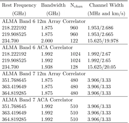
Tables 1 and 2 summarize the general observational characteristics of the ALMA
Band 6 and 7 measurements of NGC 253 presented. Three separate spectral win-dows for each frequency band in these 12m Array and ACA measurements were employed. For the Band 6 measurements each spectral window spanned frequen-cies from 217.284692 to 219.159692 GHz, 218.971025 to 220.846025 GHz, and 233.7 to 235.7 GHz. For Band 7 the three separate spectral windows spanned frequencies from 350.831145 to 352.706145 GHz, 362.482149 to 364.357149 GHz, and 363.881785 to 365.756785 GHz. For the Band 6 measurements of NGC 253 the total on-source
Table 2. Spectral Setup
Rest Frequency Bandwidth Nchan Channel Width
(GHz) (GHz) (MHz and km/s)
ALMA Band 6 12m Array Correlator
218.222192 1.875 960 1.953/2.686
219.908525 1.875 960 1.953/2.665
234.700 2.000 122 15.625/19.978
ALMA Band 6 ACA Correlator
218.222192 1.992 1024 1.992/2.67
219.908525 1.992 1024 1.992/2.65
234.700 1.938 128 15.625/20.05
ALMA Band 7 12m Array Correlator
351.768645 1.875 480 3.906/3.33
363.419649 1.875 480 3.906/3.33
364.819285 1.875 480 3.906/3.33
ALMA Band 7 ACA Correlator
351.768645 1.992 510 3.906/3.33
363.419649 1.992 510 3.906/3.33
364.819285 1.992 510 3.906/3.33
72.6 min (ACA), for a 12m:ACA on-source integration time ratio of 1:1.6. At Band 7 the total on-source integration time toward NGC 253 for each type of measurement was 34.3 min (12m Array) and 65.6 min (ACA), for a 12m:ACA on-source integration time ratio of 1:1.9. Both on-source integration time ratios are consistent with the standard integration time ratio for ALMA observations acquired in Cycle 2 of 12m
Array:ACA:TP = 1:2:4 (Mason & Brogan 2013).
Amplitude, bandpass, phase, and pointing calibration information for these
mea-surements are listed in Appendix A (Table 11). For Band 6 gain and bandpass
calibrator fluxes ranged from 253 to 688 mJy. Uncertainties in the Band 6 gain and bandpass calibrator measurements are in the range 0.4–1.7%. For Band 7 gain and bandpass calibrator fluxes ranged from 274 to 2244 mJy. Uncertainties in the Band 7 gain and bandpass calibrator measurements are with one exception in the range 0.1–3.9%. The Band 7 12m Array measurements on 2014-05-19 have higher gain calibration uncertainties which are in the range 4.3–6.4%.
At Band 6 flux calibration was effected using Uranus (28.9–34.8 Jy), Mars (78.5– 89.5 Jy), and Neptune (13.0–13.6 Jy). Band 6 flux calibrator uncertainties are
esti-mated to be 5% for Uranus (Orton et al. 2014), 10% for Mars (Perley & Butler 2013;
Weiland et al. 2011), and 10% for Neptune (M¨uller et al. 2016). For Mars our
esti-mate of the absolute flux uncertainty derives from the 1–50 GHz absolute flux (Perley
& Butler 2013) and 23–93 GHz absolute brightness temperature (Weiland et al. 2011)
have increased the nominal 5% uncertainty quoted by M¨uller et al. (2016) due to the presence of a CO absorption transition at 230.538 GHz present in the atmosphere of Neptune to 10%.
At Band 7 flux calibration was effected using J2258−2758 (390 mJy), Neptune (25.8–
27.8 Jy), and Uranus (63.8–66.6 Jy). Band 7 flux calibrator uncertainties are
esti-mated to be 10% for Neptune (M¨uller et al. 2016) and 5% for Uranus (Orton et al.
2014). As was done for our Band 6 measurements, for our absolute flux uncertainty
estimate for Neptune we have increased the nominal 5% uncertainty quoted byM¨uller
et al.(2016) due to the presence of a CO absorption transition at 345.796 GHz present
in the atmosphere of Neptune. For unknown reasons the 12m Array measurements
of NGC 253 at Band 7 employed a non-standard flux calibrator (J2258−2758). The
ALMA Calibration Catalog lists the flux uncertainty for this quasar as 15%, but no further information regarding the time period over which this uncertainty applies is provided.
All measurements were either manually or pipeline calibrated by ALMA North American Regional Center staff using the CASA reduction package. Following de-livery of each calibrated interferometric measurement group (12m Array and ACA), self-calibration was attempted to correct for residual phase errors. For all measure-ment groups at both Bands 6 and 7 one iteration of phase-only self-calibration utiliz-ing a 60 second averagutiliz-ing time was used. The bright NGC 253 continuum source at Bands 6 and 7 was used as a self-calibration source, which resulted in signal-to-noise improvement by factors of 2.9 and 1.9 in the Band 6 continuum of our 12m Array and ACA data, and by factors of 3.0 and 3.5 in the Band 7 continuum of our 12m Array and ACA data, respectively.
3. RESULTS
3.1. Imaging and Spectral Baseline Fitting
Spectral cube imaging was performed using the CASA package. Images of each self
calibrated spectral window image cube for NGC 253 were created using the clean
task within CASA. An image may be characterized by the spatial frequencies which are well represented in it; these correspond to the regions in the Fourier transform (“uv” space) of the image which were well measured by the instrument. Interferom-eters generally cover a range of spatial frequencies which are limited by the longest
and shortest baselines used in the interferometric measurement (see Table 1). Single
antennas, in principle, measure all spatial frequencies down to those corresponding to the instrument reflector diameter. Ideally, images with overlapping, well-sampled spatial frequencies can be combined to derive an image which represents all the sam-pled spatial frequencies. “Feathering” is a technique by which images are combined
in the uv plane to recover the spatial frequencies in the input images (Cotton 2017).
task feather. Table 3 lists the properties of each 12m Array, ACA, and feathered image cubes for each spectral window from our measurements of NGC 253.
Table 3. Spectral and Continuum Image Properties
Rest Frequency ∆v θmaj ×θmin@PAa RMS per Channel
(GHz) (km/s) (arcsec,arcsec,deg) (mJy/beam)
NGC 253 Band 6 12m Array
218.222192 5.5 1.52×0.87@+82.15 2.5
219.908525 5.5 1.56×0.89@+83.96 2.0
234.700 25.0 1.41×0.81@+82.28 0.9
NGC 253 Band 6 ACA
218.222192 5.5 7.55×4.70@+78.94 12.5
219.908525 5.5 7.61×4.78@+79.08 10.0
234.700 25.0 7.19×4.32@+76.34 6.0
NGC 253 Band 6 12m Array and ACA Feather
218.222192 5.5 1.52×0.87@+82.15 2.5
· · · 55 (cont) · · · 0.8
219.908525 5.5 1.56×0.89@+83.96 1.8
· · · 385 (cont) · · · 0.3
234.700 25.0 1.41×0.81@+82.28 0.9
· · · 250 (cont) · · · 0.4
NGC 253 Band 7 12m Array
351.768645 3.5 0.45×0.29@−85.64 2.0
363.419649 3.5 0.43×0.28@−85.94 2.8
364.819285 3.5 0.43×0.28@−86.00 3.0
NGC 253 Band 7 ACA
351.768645 3.5 4.99×2.48@+79.58 13.5
363.419649 3.5 4.79×2.39@+78.17 13.5
364.819285 3.5 4.78×2.39@+78.96 22.0
NGC 253 Band 7 12m Array and ACA Feather
351.768645 3.5 0.45×0.29@−85.64 2.0
· · · 35 (cont) · · · 0.9
363.419649 3.5 0.43×0.28@−85.94 3.0
· · · 35 (cont) · · · 0.8
364.819285 3.5 0.43×0.28@−86.00 3.2
· · · 35 (cont) · · · 1.5
a Continuum beam parameters are the same as their corresponding spectral
0 100 200 300 400 500 600 700 Baseline Length (m)
0 5000 10000 15000 20000 25000 30000 35000 40000
Weight per 5m Ring
Blue = ACA Data
Green = 12m Array Data
UV Weight Distribution as a Function of UV Distance
Figure 1. Annularly-averaged uv data weights as function of baseline length for the 351 GHz spectral window from our Band 7 12m Array and ACA measurements of NGC 253. The 12m Array and ACA uv data weights shown have been rescaled to place them on the same scale. This comparison suggests that the ACA data contributes minimally to the combined spatial frequency information in our imaging of NGC 253.
To assess the relative import of each contributing image cube to the combined (feathered) spectral image cube, we have plotted the uv data weights averaged over 5 m annuli in the uv-plane as a function of baseline length for corresponding 12m
Array and ACA data sets from our measurements. Figure 1 shows the
annularly-averaged uv data weights for the 12m Array and ACA measurements of our Band 7 spectral window near 351 GHz. This comparison shows that the ACA measure-ments contribute minimally to the overall spatial frequency sensitivity in our imaging measurements.
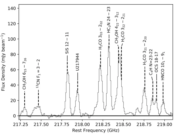
Due to the density of spectral lines in all of the spectral image cubes for NGC 253
(Figure2presents an example spectrum), spectral baseline fitting was an iterative
pro-cess using the CASA taskimcontsub. Almost all baselines were fit with zeroth order
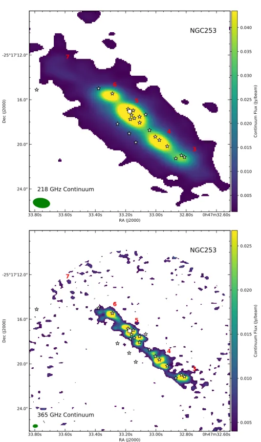
polynomials, with only a few exceptions requiring the use of first order polynomials. Visual inspections of the quality of the baseline removal for all spectral windows indi-cates good quality overall. For all but one spectral window, only 10 spectral channels are believed to be line-free (the Band 6 spectral window near 219 GHz is estimated to have 70 line-free channels). Following baseline subtraction the line-free channels from each spectral window were collapsed to form a pseudo-continuum image of NGC 253 in each spectral window. The properties of these pseudo-continuum images are listed
in Table 3 and displayed in Figure 3. Note that the RMS noise values listed for
217.25 217.50 217.75 218.00 218.25 218.50 218.75 219.00
Rest Frequency (GHz)
0
20
40
60
80
100
120
140
Flu
x D
en
sit
y (
m
Jy
be
am
1
)
CH
3OH
6
157
2613
CN
F
1=
3
2
SiS
1
2
11
U217944
H
2CO
3
032
02HC
3N
24
23
CH
3OH
4
223
12H
2CO
3
222
21H
2CO
3
212
20C
4H
N=
23
-2
2
OCS 18-17
HN
CO
1
0
19
1Figure 2. Sample spectrum from our NGC 253 Band 6 measurements centered at a rest fre-quency of 218.222192 GHz. Shown is the spectrum centered on Region 6 and averaged over a one arcsecond area and spectrally smoothed to 10 km/s. Identified molecular transitions are indicated.
As it will be convenient to interchange between flux and brightness temperature,
we will use the general relation between the flux density of a source (Sν) with solid
angle Ω and its brightness temperature (TB):
Sν =
2kν2
c2
Z
TB(Ω)dΩ (1)
Note that Equation 1 assumes that the Rayleigh-Jeans approximation (hν kT)
applies. Assuming R
TBdΩs =TBΩs with Ωs equal to the synthesized gaussian beam
solid angle ΩB =
πθmajθmin
4 ln 2 in Equation 1 results in the following general relation
between flux density and measured brightness temperature for a point source:
TB(K)'13.6
300
ν(GHz)
2
Sν(J y)
θmaj(arcsec)θmin(arcsec)
(2)
3.2. Spatial Component Identification
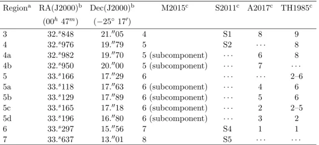
Using the continuum images described in Section3.1, we have fit single-component
elliptical gaussians to each of the continuum peaks in these images. Table 4lists the
0h47m32.60s 32.80s
33.00s 33.20s
33.40s 33.60s
33.80s
RA (J2000) 24.0"
20.0" 16.0" -25°17'12.0"
Dec (J2000)
1
2
3
4
5
6
7
8
9
218 GHz Continuum
NGC253
0.005 0.010 0.015 0.020 0.025 0.030 0.035 0.040
Continuum Flux (Jy/beam)
0h47m32.60s 32.80s
33.00s 33.20s
33.40s 33.60s
33.80s
RA (J2000) 24.0"
20.0" 16.0" -25°17'12.0"
Dec (J2000)
1
2
3
4
5
6
7
8
9
10
365 GHz Continuum
NGC253
0.005 0.010 0.015 0.020 0.025
Continuum Flux (Jy/beam)
Figure 3. Band 6 (218 GHz with RMS = 0.8 mJy/beam; top) and Band 7 (365 GHz with RMS = 1.5 mJy/beam; bottom) continuum images of NGC 253, shown on the same spatial scale and range. Red numbers indicate the locations of the dense molecular emission regions
identified byLeroy et al.(2015, Table4). White black-bordered markers locate the positions
of the 2 cm radio continuum emission peaks (Ulvestad & Antonucci 1997), with a square
indicating the position of the strongest radio continuum peak identified by Turner & Ho
Table 4. NGC 253 Continuum Source Positions and Component Correspondence
Regiona RA(J2000)b Dec(J2000)b M2015c S2011c A2017c TH1985c
(00h 47m) (−25◦ 170)
3 32.s848 21.0005 4 S1 8 9
4 32.s976 19.0079 5 S2 · · · 8
4a 32.s982 19.0070 5 (subcomponent) · · · 6 8
4b 32.s950 20.0000 5 (subcomponent) · · · 7 · · ·
5 33.s166 17.0029 6 · · · 2–6
5a 33.s118 17.0063 6 (subcomponent) · · · 4 6
5b 33.s129 17.0089 6 (subcomponent) · · · 5 6
5c 33.s165 17.0018 6 (subcomponent) · · · 2 2–5
5d 33.s196 16.0080 6 (subcomponent) · · · 3 2
6 33.s297 15.0056 7 S4 1 1
7 33.s637 13.0001 8 S5 · · · ·
aNomenclature adopts Leroy et al.(2015) component numbering.
b Position errors are all<0.2500.
c M2015:Meier et al. (2015), S2011:Sakamoto et al. (2011), A2017:Ando et al. (2017),
TH1985:Turner & Ho(1985).
noted by Leroy et al.(2015),Meier et al. (2015),Sakamoto et al. (2011),Ando et al.
(2017), and Turner & Ho (1985). Note that components 4 and 5 split into multiple
components in our higher-resolution Band 7 measurements, as previously noted by
Ando et al.(2017). In the following we will use the regions noted in Table4as spatial
reference positions for further analysis of the spectral emission properties within the nuclear disk of NGC 253.
3.3. Spatial Component Hydrogen Column Density and Mass
Using the peak continuum flux measurements derived from our spatial gaussian fits
to our continuum images (Section 3.2), and assuming that the continuum emission
is dominated by thermal dust emission, we have calculated the hydrogen column densities and masses using the well-worn dust emission assumptions elucidated by
Hildebrand (1983). Assuming that the hydrogen column densities and masses are
dominated by molecular hydrogen, the total column density and mass of hydrogen is given by:
N(H2)'7.0×10²²Rgd
λ(mm)
0.4
β
TR(K) Td(K)
cm−2 (3)
M(H2)'2×10⁻⁴Rgd
λ(mm)
0.25
β+3
D2(kpc)Sν(J y) exp
14.4
λ(mm)Td(K)
−1
M
where we have assumed optically-thin dust emission (TR=Td[1−exp(−τλ)]'Tdτλ)
and parameterized the gas-to-dust mass ratio as Rgd. The assumption of
optically-thin dust emission appears to be justified given the moderate continuum brightness
temperatures of ∼ 0.5 K that we measure. This optically-thin assumption is also
consistent with the submillimeter through infrared dust continuum measurements
presented in P´erez-Beaupuits et al. (2018). The other variables are the wavelength
of observation (λ) in millimeters, the dust emissivity power law (β), the radiation
temperature corresponding to the measured continuum flux in Kelvin (TR), and the
dust temperature (Td), also in Kelvin. We also use Equation 2 to convert our
mea-sured continuum fluxes (Sν) to radiation temperatures (TR) assuming the spatial
resolutions associated with each continuum image. Assuming then that Rgd = 150,
β = 1.5, and Td = 35 K (see discussion in Leroy et al. 2015, Section 3.1.1), with the
associated region dust continuum fluxes, we derive the hydrogen column densities and
masses listed in Table 5. The GMC hydrogen masses we derive are consistent with
those measured by Leroy et al. (2015), and the sum of our GMC hydrogen masses
is consistent with the total CMZ hydrogen mass of 4.5±1.3×10⁸M
measured by
P´erez-Beaupuits et al. (2018).
Our assumption of Rgd = 150 follows that of Leroy et al. (2015) and Weiß et al.
(2008), which leverages the elemental (carbon through nickel) depletion analysis
pre-sented inDraine (2011), which itself uses the Milky Way elemental depletion analysis
presented inJenkins (2009). The average depletion of all sightlines analyzed by
Jenk-ins (2009) is F∗ = 0.36, which implies a value for the gas-to-dust mass ratio of the
diffuse Milky Way ofRgd= 150. Even though it is not clear if a diffuse gas Milky Way
value for Rgd is appropriate to the dense CMZ of NGC 253, it is the only properly
calibrated, through line-of-sight UV absorption measurements, value for this quantity. In order to calculate molecular abundances using our total molecular column
densi-ties (Section6), we average our GMC-specific hydrogen column densities per receiver
band over any sub-components which comprise a main GMC in Table 5. These
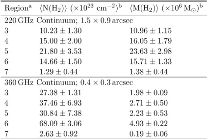
aver-aged hydrogen column densities (and masses) are listed in Table6. As will be done for
our calculations of the total molecular column density (Section 6), the uncertainties
associated with each hydrogen column density and mass represent the larger of the statistical uncertainty and the standard deviation of the individual column densities or masses derived. These averaged hydrogen column densities will be used to derive molecular abundances within the GMCs of NGC 253.
4. ANALYSIS
4.1. Spectral Line Identification
Molecular spectral line identification within each spectral window of our NGC 253 measurements was done in two steps. In a first step the ALMA Data-Mining Toolkit
(ADMIT; Teuben et al. 2015) was used to search for the most appropriate
Table 5. NGC 253 GMC Hydrogen Column Densities and Masses
Regiona Sν (mJy) N(H2) (×1023cm−2)b M(H2) (×106M)b
218 GHz Continuum; 1.52×0.87 arcsec
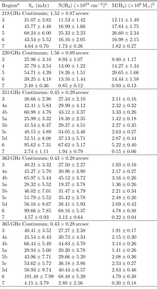
3 31.07±3.82 11.53±1.42 12.11±1.49
4 45.77±4.48 16.99±1.66 17.84±1.75
5 68.24±6.00 25.33±2.23 26.60±2.34
6 43.54±5.52 16.16±2.05 16.98±2.15
7 4.64±0.70 1.73±0.26 1.82±0.27
220 GHz Continuum; 1.56×0.89 arcsec
3 25.96±3.10 8.93±1.07 9.80±1.17
4 37.79±3.54 13.00±1.22 14.27±1.34
5 54.71±4.39 18.26±1.51 20.65±1.66
6 38.25±4.18 13.16±1.44 14.44±1.58
7 2.48±0.36 0.85±0.12 0.93±0.13
351 GHz Continuum; 0.45×0.29 arcsec
3 38.66±2.98 27.34±2.10 2.11±0.16
4a 42.41±5.83 29.99±4.12 2.32±0.32
4b 60.98±4.76 43.12±3.37 3.33±0.26
5a 25.99±3.32 18.38±2.35 1.42±0.18
5b 41.54±6.37 29.37±4.51 2.27±0.35
5c 48.15±4.89 34.05±3.46 2.63±0.27
5d 52.51±8.08 37.13±5.71 2.87±0.44
6 95.62±7.31 67.62±5.17 5.22±0.40
7 2.74±1.11 1.94±0.79 0.15±0.06
363 GHz Continuum; 0.43×0.28 arcsec
3 40.21±3.32 27.50±2.27 1.93±0.16
4a 45.27±5.70 30.96±3.90 2.17±0.27
4b 65.97±5.44 45.12±3.72 3.16±0.26
5a 28.32±5.52 19.37±3.78 1.36±0.26
5b 46.02±7.01 31.47±4.79 2.21±0.34
5c 51.79±5.52 35.42±3.78 2.48±0.26
5d 56.16±8.67 38.41±5.93 2.69±0.42
6 99.66±7.85 68.16±5.37 4.78±0.38
7 4.57±0.93 3.13±0.64 0.22±0.04
365 GHz Continuum; 0.43×0.28 arcsec
3 40.41±3.52 27.27±2.38 1.91±0.17
4a 45.54±6.43 30.73±4.34 2.15±0.30
4b 66.44±5.49 44.83±3.70 3.14±0.26
5a 29.94±5.60 20.20±3.78 1.41±0.26
5b 43.96±7.71 29.66±5.20 2.08±0.36
5c 53.62±5.72 36.18±3.86 2.53±0.27
5d 59.93±9.74 40.44±6.57 2.83±0.46
6 101.48±7.99 68.48±5.39 4.79±0.38
7 4.15±3.79 2.80±2.56 0.20±0.18
aNomenclature adopts Leroy et al.(2015) component numbering.
b Assuming R
Table 6. NGC 253 Average GMC Hydrogen Column Den-sities and Masses
Regiona hN(H2)i(×1023 cm−2)b hM(H2)i (×106M)b
220 GHz Continuum; 1.5×0.9 arcsec
3 10.23±1.30 10.96±1.15
4 15.00±2.00 16.05±1.79
5 21.80±3.53 23.63±2.98
6 14.66±1.50 15.71±1.33
7 1.29±0.44 1.38±0.44
360 GHz Continuum; 0.4×0.3 arcsec
3 27.38±1.31 1.98±0.09
4 37.46±6.93 2.71±0.50
5 30.84±7.38 2.23±0.53
6 68.09±3.06 4.93±0.22
7 2.63±0.92 0.19±0.06
aNomenclature adoptsLeroy et al.(2015) component
num-bering.
b Assuming R
gd= 150, Td= 35 K, τd1, β = 1.5, and D
= 3.5 Mpc.
of NGC 253. Once an initial set of molecular species was identified, residual species within each spectral window were identified by-eye using lists of line rest frequencies
(Lovas 1992; M¨uller et al. 2001) and anticipated general abundances for potential
species. Table 12in Appendix B lists the molecular transitions and frequencies
mea-sured toward NGC 253.
The Band 6 low spectral resolution spectral window centered at a rest frequency of 234.7 GHz was anticipated to be line-free, and thus would have served as a sensitive continuum measurement. It was determined, though, that spectral lines existed in this spectral window with rest frequencies near 234.69 and 235.15 GHz. These spectral line
frequencies are consistent with CH3OH 42−51 A at 234683.39 MHz and/or CH3OH
5−4−6−3 E at 234698.45 MHz.
4.2. Spectral Line Signal Extraction and Spatial Component Fitting
In order to extract integrated spectral line intensities from our measurements we
have developed a python script, calledCubeLineMoment2, which uses a series of
spec-tral and spatial masks to extract integrated intensities for a defined list of target
spectral frequencies. CubeLineMoment makes extensive use of spectral-cube3.
The masking process begins by selecting a bright spectral line whose velocity struc-ture is representative of the emission across the galaxy. Preferably, it should be
maximally inclusive, such that all other lines emit over a smaller area in position-position-velocity (PPV) space, which here has right ascension, declination and helio-centric velocity as axes. Various images are computed based on this line, including noise, peak intensity, position of peak intensity, and second moment (velocity
disper-sion). The CO 2−1 and H2CO 515−414 transitions were found to be appropriate
choices for the bright “tracer” transitions in our Band 6 and 7 spectral windows, respectively.
These maps are then converted into a PPV mask cube by producing Gaussian profiles at each spatial pixel with peak intensity, centroid, and width defined by the appropriate masks. The Gaussians are sampled onto the PPV grid defined by the target emission line. For each spatial pixel, spectral pixels are masked-out below the
1-σlevel evaluated on the model Gaussian. By evaluating only on the model Gaussian,
we exclude pixels above 1-σ at other parts of the spectrum, which otherwise would
contribute significantly to the included region. The mask is then applied to the target emission line data cube, and moment 0, 1, and 2 maps are produced.
Integrated spectral line intensity images derived from ourCubeLineMomentanalysis
are listed in Appendix C. In order to associate spectral line integrated intensities
with each of the spatial components noted both in previous and the current
mea-surements, we have used thegaussfit catalog4 application, which usespyspeckit5
to perform gaussian fits of the spatial molecular spectral line components associated
with the regions listed in Table 4. As a characterization of the high-density
compo-nent structure within the NGC 253 nucleus, and to provide an example of the spatial
gaussian fits performed, Table7 lists the derived averaged peak position and size for
the nuclear regions derived from our H2CO 303−202, 321−220, 515−414, 505−404,
524−423, 523−422, 53−43and 54−446 integrated intensity images. We have compared
the derived peak position for each H2CO component to those which correspond to
positions derived from our Band 6 and 7 dust continuum and the spectral line
mea-surements of Leroy et al. (2015), Meier et al. (2015), Sakamoto et al. (2011), Ando
et al.(2017), andTurner & Ho(1985) (Table4). We find that with but one exception,
all peak H2CO positions are consistent within respective measurement uncertainties
with their corresponding ALMA Band 6 and 7 continuum positions, and with com-ponent positions derived from the earlier works listed. For the one exception, Region
5, the H2CO position differs by (∆RA,∆Dec) = (+0.64,+0.69) arcsec ((11,12) pc)
from its reference position. The position for Region 5 is derived from our Band 6
measurements, whose spatial resolution is θmaj ×θmin ' 1.5×0.9 arcsec). Region
5 is also known to have substructure in higher-resolution measurements (including our Band 7 imaging), and has been suggested as a component which suffers from
self-absorption in lower-excitation molecular spectral line measurements (Meier et al.
4https://github.com/radio-astro-tools/gaussfit catalog 5https://pyspeckit.readthedocs.io/
6Since the 5
2015). Even though real molecular abundance gradients within Region 5 cannot be excluded, the currently most plausible explanation for this position shift between our
H2CO and dust continuum plus previous low-excitation molecular emission
measure-ments is a complex emission structure below the spatial resolution and sensitivity of our measurements.
Table 7. Averaged Gaussian Fits to NGC 253 Formaldehyde Components
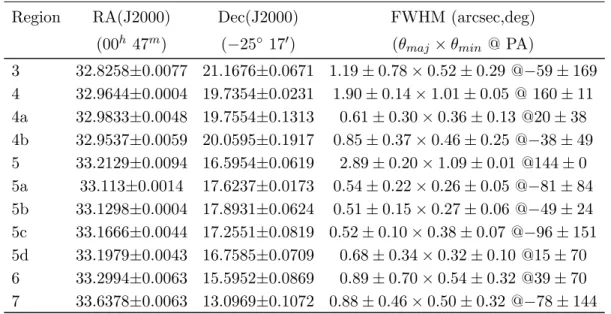
Region RA(J2000) Dec(J2000) FWHM (arcsec,deg)
(00h 47m) (−25◦ 170) (θmaj×θmin @ PA)
3 32.8258±0.0077 21.1676±0.0671 1.19±0.78×0.52±0.29 @−59±169
4 32.9644±0.0004 19.7354±0.0231 1.90±0.14×1.01±0.05 @ 160±11
4a 32.9833±0.0048 19.7554±0.1313 0.61±0.30×0.36±0.13 @20±38
4b 32.9537±0.0059 20.0595±0.1917 0.85±0.37×0.46±0.25 @−38±49
5 33.2129±0.0094 16.5954±0.0619 2.89±0.20×1.09±0.01 @144±0
5a 33.113±0.0014 17.6237±0.0173 0.54±0.22×0.26±0.05 @−81±84
5b 33.1298±0.0004 17.8931±0.0624 0.51±0.15×0.27±0.06 @−49±24
5c 33.1666±0.0044 17.2551±0.0819 0.52±0.10×0.38±0.07 @−96±151
5d 33.1979±0.0043 16.7585±0.0709 0.68±0.34×0.32±0.10 @15±70
6 33.2994±0.0063 15.5952±0.0869 0.89±0.70×0.54±0.32 @39±70
7 33.6378±0.0063 13.0969±0.1072 0.88±0.46×0.50±0.32 @−78±144
Table 8 lists the spectral line integrated intensities derived from the
CubeLineMoment output and gaussfit catalog gaussian fit analysis from all
de-tected transitions which are not significantly blended and whose derived integrated
intensity is larger than 2σ. Full-width half-maximum (FWHM) line widths derived
from this analysis range from ∼ 50 to ∼ 80 km/s for most of our unblended
T able 8 . NGC 253 In tegrated Sp ectral Line In tensities (Jy km/s) a T ransition Region 3 Region 4 Region 5 Region 6 Region 7 13 CO 2 − 1 16.15 ± 4.11 19.51 ± 4.00 (3.30) 26.53 ± 4.55 11.92 ± 3.20 C 18 O 2 − 1 6.80 ± 1.60 7.17 ± 1.34 (1.07) 11.91 ± 1.67 4.48 ± 1.09 13 CN, F1 =3-2 (0.12) 1.42 ± 0.17 (0.15) 1.29 ± 0.13 (0.04) SiS 12 − 11 2. 22 ± 0.32 2.37 ± 0.30 (0.29) 3.27 ± 0.37 1.42 ± 0.11 SO 65 -54 1.46 ± 0.19 2.49 ± 0.20 1.70 ± 0.22 4.68 ± 0.32 0.94 ± 0.05 SO 2 422 − 313 1.05 ± 0.11 0.94 ± 0.10 0.54 ± 0.09 1.32 ± 0.15 0.20 ± 0.07 SO 2 533 − 422 0.31 ± 0.05 4a:0.25 ± 0.06, 4b:0.66 ± 0.12 5a:0.15 ± 0.03, 5b:0.25 ± 0.04, 5c:0.28 ± 0.08, 5d:0.38 ± 0.13 0.90 ± 0.04 (0.04) SO 2 14 4 , 10 − 14 3 , 11 0.21 ± 0.07 4a:0.30 ± 0.07, 4b:0.80 ± 0.24 5a:0.37 ± 0.10, 5b:(0.09), 5c:0.99 ± 0.12, 5d:0.44 ± 0.08 1.34 ± 0.08 (0.03) HNC 4 − 3 3.90 ± 0.81 4a:17.99 ± 1.27, 4b:(1.61) 5a:6.03 ± 2.22, 5b:3.62 ± 2.16, 5c:6.05 ± 1.47, 5d:(3.45) 28.77 ± 1.38 1.54 ± 0.22 HNC 4 − 3 ν2 = 1 f 0.68 ± 0.07 4a:1.81 ± 0.07, 4b:(0.07) 5a:1.21 ± 0.13,
5b:(0.17), 5c:(0.09), 5d:(0.56)
5. KINETIC TEMPERATURE DERIVATION USING FORMALDEHYDE
As described byMangum & Wootten(1993), the Formaldehyde molecule possesses
structural properties which allow for its rotational transitions to be used as probes of
the kinetic temperature in dense molecular gas environs. H2CO is a slightly
asymmet-ric rotor molecule, so that its energy levels are defined by three quantum numbers: total angular momentum J, the projection of J along the symmetry axis for a limiting
prolate symmetric top, K−1, and the projection of J along the symmetry axis for a
limiting oblate symmetric top, K+1. The H2CO energy level diagram which shows all
energy levels below 300 K is shown in Figure 12 of Mangum & Wootten (1993).
For radiative excitation in a symmetric rotor molecule, dipole selection rules
dic-tate that ∆K = 0. Transitions between energy levels when ∆K6=0 can only occur
via collisional excitation. This, then, is the fundamental reason why symmetric rotor molecules are tracers of kinetic temperature in dense molecular clouds. A comparison between the energy level populations from different K-levels within the same molec-ular symmetry species (ortho or para) should allow a direct measure of the kinetic
temperature in the gas. The asymmetry in H2CO (κ=−0.96) makes it structurally
similar to a prolate symmetric rotor molecule (κ=−1.0). Therefore, measurements
of the relative intensities of two transitions whose K-levels originate from the same ∆J = 1 transition provide a direct measure of the kinetic temperature.
To connect the kinetic temperature in the dense nuclear gas in starburst galaxies to the intensity of molecular transitions which originate from these nuclei, one needs to solve for the coupled statistical equilibrium and radiative transfer equations. A simple solution to these coupled equations is afforded by the Large Velocity Gradient
(LVG) approximation (Sobolev 1960). The detailed properties of our
implementa-tion of the LVG approximaimplementa-tion are described in Mangum & Wootten (1993). From
the Mangum & Wootten (1993) summary of the uncertainties associated with LVG
model results, we note that uncertainties in the collisional excitation rates (Green
1991), which can be as high as 50% for state-to-state rates, are not included in our
analysis uncertainties. This contribution to the uncertainties of our derived physical conditions is traditionally ignored, and we only mention it here to provide context to our analysis. The simplified solution to the radiative transfer equation which the LVG approximation provides allows for a calculation of the global dense gas properties in a range of environments.
We have applied our LVG model formalism to the unblended H2CO transitions
mea-sured toward NGC 253. With the nine transitions for which we have meamea-sured
inte-grated intensities (Table8) we can form five unique H2CO transition ratios which can
be used to derive the kinetic temperature in the dense nuclear regions of NGC 253.
The analysis of the limits in kinetic temperature, volume density, and H2CO
col-umn density to our measured H2CO kinetic temperature sensitive ratios derived by
Mangum & Wootten (1993) are directly applicable to our NGC 253 measurements.
in a molecular cloud core, the following integrated intensity ratios measure kinetic
temperature to an uncertainty of .25 %:
• Sdv(303−202)
Sdv(321−220) when TK . 50 K and N(para-H2CO)/∆v . 10
13.5cm−2/(km s−1).
This rule also applies to the same ratio involving the 322−221 transition.
• Sdv(505−404)
Sdv(523−422) when TK . 75 K and N(para-H2CO)/∆v . 10
14.0cm−2/(km s−1).
This rule also applies to the same ratio involving the 524−423 transition.
• Sdv(524−423)
Sdv(54−44) when TK .150 K and N(para-H2CO)/∆v.10
14.5cm−2/(km s−1).
• Sdv(515−414)
Sdv(53−43) when TK .100 K and N(ortho-H2CO)/∆v .10
14.0cm−2/(km s−1)
and to an upper limit, defined as the point at which the uncertainty in TK becomes
50%, of:
• TK . 150 K for Sdv(303
−202)
Sdv(321−220). This rule also applies to the same ratio involving
the 322−221 transition.
• TK . 200 K Sdv(505
−404)
Sdv(523−422). This rule also applies to the same ratio involving the
524−423 transition.
• TK . 300 K SdvSdv(5(524−423)
4−44) . This rule also applies to the same ratio involving the
523−422 transition.
• TK .250 K
Sdv(515−414) Sdv(53−43) .
for the limits to the column densities per line width (FWZI) listed.
Due to velocity blending with the HNC 4−3 transition the H2CO 505−404transition
cannot be used as a reliable kinetic temperature diagnostic in NGC 253. We rely then
on the Sdv(303−202)
Sdv(321−220),
Sdv(515−414) Sdv(53−43) ,
Sdv(524−423)
Sdv(54−44) , and
Sdv(523−422)
Sdv(54−44) ratios to derive kinetic
temperature images of the NGC 253 CMZ.
Over the range of H2CO volume densities and kinetic temperatures appropriate to
our NGC 253 measurements our measured kinetic temperature sensitive integrated
in-tensity ratios are relatively insensitive to changes in H2CO column density (Mangum
& Wootten 1993). Therefore, we have interpolated our measured integrated
in-tensity ratios onto our LVG model grid assuming log(N(species−H2CO)/∆v) =
12.5 cm−2/(km s−1) and log(n(H
2)) = 5.0 (Mangum et al. 2013a), where “species”
is ortho or para. We have also applied the sensitivity limits listed above to properly
identify the upper limit to the kinetic temperature sensitivity for each H2CO
transi-tion ratio. This then allows us to convert our measured H2CO integrated intensity
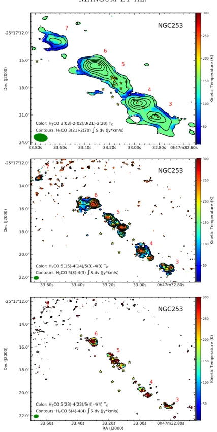
ratios to kinetic temperatures. Figure 4 shows the results deduced from the above
mentioned ratios and the resulting LVG model interpolation.
From our NGC 253 kinetic temperature images shown in Figure 4 we can conclude
that:
• Based on the Sdv(303−202)
Sdv(321−220) and
Sdv(515−414)
Sdv(53−43) ratios the kinetic temperature ranges
22 Mangum et al.
0h47m32.60s 32.80s
33.00s 33.20s 33.40s 33.60s 33.80s
RA (J2000) 24.0"
21.0" 18.0" 15.0" -25°17'12.0"
Dec (J2000)
1 2
3 4 5
6 7
8 9
Color: H2CO 3(03)-2(02)/3(21)-2(20) TK Contours: H2CO 3(21)-2(20) S dv (Jy*km/s)
NGC253
50 100 150 200 250 300
Kinetic Temperature (K)
0h47m32.80s 33.00s
33.20s 33.40s
33.60s
RA (J2000) 22.0"
20.0" 18.0" 16.0" 14.0" -25°17'12.0"
Dec (J2000)
1 2
3 4
5 6 7
8 9 10
Color: H2CO 5(15)-4(14)/5(3)-4(3) TK Contours: H2CO 5(3)-4(3) S dv (Jy*km/s)
NGC253
50 100 150 200 250 300
Kinetic Temperature (K)
0h47m32.80s 33.00s
33.20s 33.40s
33.60s
RA (J2000) 22.0"
20.0" 18.0" 16.0" 14.0" -25°17'12.0"
Dec (J2000)
1 2
3 4
5 6 7
8 9 10
Color: H2CO 5(23)-4(22)/5(4)-4(4) TK Contours: H2CO 5(4)-4(4) S dv (Jy*km/s)
NGC253
50 100 150 200 250 300
Kinetic Temperature (K)
Figure 4. Kinetic temperature images derived from H2CO integrated intensity ratios: Sdv(303−202)
Sdv(321−220) (top),
Sdv(515−414)
Sdv(53−43) (middle),
Sdv(524−423)
Sdv(54−44) (bottom). Note that the appropriate
upper sensitivity limit to the kinetic temperature scale has been applied based on the
discussion in Section5: 150 K (top), 250 K (middle), and 300 K (bottom). The synthesized
beam is displayed in the lower-left of each panel. Red numbers indicate the locations of the
dense molecular transition regions identified by Leroy et al. (2015, Table 4). Yellow stars
locate the positions of the 2 cm radio continuum emission peaks (Ulvestad & Antonucci
1997), with a square indicating the position of the strongest radio continuum peak identified
byTurner & Ho(1985) (TH2: RA(J2000) = 00h47m33s.18, Dec(J2000) =−25◦1701600.93).
Contour levels are 0.25, 0.50, 1.0, 1.5, 2.0, and 2.5 Jy*km/s (H2CO 321−220); 0.10, 0.25,
• On smaller physical scales, .1 arcsec (.16 pc), our Sdv(515−414) Sdv(53−43) and
Sdv(524−423) Sdv(54−44)
ratios indicate that the kinetic temperature is greater than 300 K.
An analysis of the H2CO 110−111 and 211−212 emission toward NGC 253 (Mangum
et al. 2013a) measured volume densities n(H2)≥104−5cm−3. Furthermore, the
effec-tive critical density (Shirley 2015) for the H2CO transitions considered in the current
analysis is n(H2) & 104cm−3. Our dense gas imaging of NGC 253 has therefore
re-vealed volume densities that are greater than 104−5cm−3, our dense gas imaging of
NGC 253 has revealed the existence of very high kinetic temperatures within the dense star-forming gas which encompasses a large area within the starburst nucleus
of NGC 253. In Section7we will investigate the potential sources for these high dense
gas kinetic temperatures.
5.1. Comparison to Previous Kinetic Temperature Measurements
As was summarized inMangum et al.(2008),Mangum et al.(2013a), andMangum
et al. (2013b) numerous measurements of dense-gas molecular tracers have pointed
to the existence of multiple temperature components in NGC 253. Three of the more
recent studies of the nuclear kinetic temperature structure within NGC 253 (Mangum
et al. 2013b; Gorski et al. 2017; P´erez-Beaupuits et al. 2018) suggest the existence of
at least two kinetic temperature components:
• A warm component with TK '75 K
• A hot component with TK &150 K
A third cooler component with TK ' 40−50 K is also required by the dust and gas
spectral energy distribution fits of P´erez-Beaupuits et al. (2018), though it may be
difficult to distinguish this component from the cooler wings of a 75 K component in many of the previous high-excitation molecular spectral line measurements. These previous dense molecular gas kinetic temperature measurements are consistent with
our H2CO derived kinetic temperatures in NGC 253. The warm component measured
in previous low spatial resolution studies is associated with dense gas on ∼ 80 pc
scales, while the hot component appears to originate in dense gas on .16 pc scales.
6. MOLECULAR SPECTRAL LINE COLUMN DENSITY
In order to measure the relative abundances of the molecular species sampled by our ALMA imaging of NGC 253 we need to calculate the molecular column density for each species. In all but a handful of species we have sampled only one transition, which dictates that we perform a rather simplistic analysis of the molecular column density. With little information beyond the intensity and spatial distribution of each measured transition, to calculate molecular column densities we assume a kinetic
temperature derived from our H2CO measurements (see Section 5) in the
the kinetic temperature, and that the source filling factor is unity, from Mangum &
Shirley(2015) we adopt the total molecular column density in the optically-thin limit
with Tex Tbg given by:
Ntotthin=
3k
8π3Sµ2νR
i
Qrot gJgKgI
exp
Eu
TK
Z
TBdv cm−2, (5)
whereS is the transition line strength, µis the molecular dipole moment in Debye,ν
is the transition frequency in GHz,Ri is the relative transition intensity (for hyperfine
transitions),gJ,gI, andgK are the rotational, nuclear spin, and K degeneracies,Eu is
the transition upper energy level in Kelvin, TK is the kinetic temperature in Kelvin,
TB is the measured transition brightness temperature, and Qrot is the rotational
partition function:
Qrot =
∞
X
J=0 J
X
K=−J
gKgI(2J+ 1) exp
−EJ K Trot
(6)
for linear (where the summation over K is removed), symmetric, and
slightly-asymmetric rotor molecules. EJ K represents the energy above the ground state in
Kelvin for a transition with quantum numbers (J,K). We assume that the rotational
temperature, Trot, is equal to the kinetic temperature. Inserting Equation 2 for TB
into Equation5 results in the following:
Ntotthin'
2.04×10²⁰Qrotexp
Eu TK
R
Sν(J y)dv(km/s)
Sµ2(Debye)ν3(GHz)R
igJgKgIθmaj(arcsec)θmin(arcsec)
cm−2 (7)
To check whether our assumption of optically-thin emission is reasonable, we com-pared our measured spectral line peak intensities to those derived from an LVG model
prediction of those intensities. For example, our measured13CO and C18O 3−2
inte-grated intensities are∼10−20 Jy km/s (Table8), with FWHM of∼50 km/s. For an
LVG model which assumes TK = 150 K (Section 5), n(H2) = 104cm−3, and N(13CO
or C18O) = 1017cm−2 (Table9), we find that τ '0.1 for both13CO and C18O 3−2,
with predicted brightness temperatures similar to those that we measure.
Further-more, if one assumes a lower kinetic temperature of 50 K in these LVG calculations,τ
increases modestly to ' 0.3. Similar estimates using LVG model calculations which
use our measured peak brightness temperatures and column densities to estimate transition optical depths indicate that most of our measurements are well within the optically-thin regime, and only reach moderate optical depths in a few cases. Two
such moderate optical depth cases are the H2CO 303−202 and 322−221 transitions,
for which τ '0.8 and 0.4, respectively. As the H2CO column density is based on a
sample of seven transitions (Table 9), the moderate optical depths within these two
transitions is unlikely to significantly affect the total H2CO column density derived.
Usingθmaj,θmin, and
R
Sν(J y)dv(km/s) from Table8and the spectral line
(S), transition degeneracies (gJ, gK, gI), and partition function values at
representa-tive kinetic temperatures (Qrot(T); Table12), we calculateNtotthin in Table9using the
indicated variable values and assuming TK = 150 K. We have chosen TK = 150 K as
the representative kinetic temperature for our molecular column density calculations
as it accounts for both the warm gas measured on GMC (∼80 pc) spatial scales, and
the hot gas measured on smaller (.16 pc) scales (see Section 5).
Note that to scale these total optically-thin molecular column densities to an
as-sumed kinetic temperature other than 150 K, one simply needs to apply Equation 8
to the total molecular column densities listed in Table 9:
Nthin tot (TK1) Nthin
tot (TK2)
=Qrot(TK1)
Qrot(TK2)
exp
Eu TK1
− Eu
TK2
'
TK1 TK2
n2
exp
Eu TK1
− Eu
TK2
(8)
where we have used the fact that, to a very good approximation, Qrot(TK) ∝ T
n 2 K,
where n = 2 for linear molecules and n = 3 for symmetric and slightly-asymmetric
rotor molecules (see Mangum & Shirley 2015, Section 7).
When multiple transitions are available (indicated by the Ntranscolumn in Table 9),
a spatially-averaged molecular column density is listed whose uncertainty is the larger of the statistical uncertainty and the standard deviation of the individual transition column densities derived. Spatial averaging is done in order to include measurements from both Bands 6 and 7, in that we have averaged over the Band 7 subcomponents
within Regions 4 and 5. In Section7.2we will compare the relative abundances of the
7. WHAT DRIVES THE HIGH KINETIC TEMPERATURES IN NGC 253?
As was shown in Section 5 the kinetic temperature within the starburst nucleus
of NGC 253 is ∼ 50 to & 150 K on ∼ 80 pc scales, and rises to kinetic
tempera-tures greater than 300 K on . 16 pc scales. NH3 measurements yield similar values
(Mangum et al. 2013b). Furthermore, note that the Galactic CMZ possesses
simi-larly high kinetic temperatures over GMC (∼80 pc) size scales (Ginsburg et al. 2016;
Ao et al. 2013). Mills & Morris (2013), from observations of high energy level NH3
absorption, find evidence for an even hotter gas component (TK > 350 K) that is
widespread in the Galactic CMZ. This component most likely originates in a lower
density gas component that is not sampled by our H2CO data, which exclusively
trace dense gas. Our TK > 300 K gas thus is not a counterpart of the Galactic
CMZ dilute gas component. What physical processes can maintain such high kinetic temperatures?
As we discussed previously in the context of the high dense gas kinetic temperatures
measured using NH3 emission within a sample of starburst galaxies (Mangum et al.
2013b), high kinetic temperatures can be generated by cosmic ray (CR) and/or
me-chanical heating. CR heating can be effective at high column densities due to the small
(∼ 3×10⁻²⁶cm−2) H
2 CR dissociation cross section (P´erez-Beaupuits et al. 2018).
As noted in Mangum et al. (2013b), adapted chemical Photon Dominated Region
(PDR) models have been used by a number of groups (e.g. Bayet et al. 2011;
Mei-jerink et al. 2011) to study the effects of CR and mechanical heating on the chemical
abundances within starburst galaxies. In these models, kinetic temperatures ranging up to 150 K can be generated by injecting varying amounts of CR and/or mechanical
energy. For example, in the CR plus mechanical heating models of Meijerink et al.
(2011), TK '150 K is attained for a mechanical heating rate of 3×10⁻¹⁸erg cm−3s−1
in a high density (n(H2) = 105.5cm−3) high column density (N(H2)>1022cm−2)
envi-ronment with CR rates ranging from 5×10⁻¹⁷−5×10⁻¹⁴s−1. In order to distinguish
between different physical processes which can produce the signatures of CR and/or mechanical energy, in the following we evaluate the radiative and chemical diagnostics of energy input within starburst galaxies.
7.1. Radio, Near-Infrared, and X-ray Diagnostics of Dense Gas Heating
Radio wavelength measurements (Turner & Ho 1985; Ulvestad & Antonucci 1997;
Brunthaler et al. 2009) ranging fromλ= 1.3 to 20 cm have identified over 60 individual
compact continuum sources within the NGC 253 central molecular zone. Figures 3
through 25 show the locations of the compact 2 cm continuum sources identified
by Ulvestad & Antonucci (1997). The brightest of these radio continuum sources
(S(2 cm) ' 30 mJy/beam within θ ' 0.05 arcsec) is located at the dynamical center
of NGC 253 and has been suspected to be either a low-luminosity active galactic
nucleus (LLAGN) or a compact supernova remnant (Turner & Ho 1985;Ulvestad &
“TH2” in this article and indicated by a filled-square in the figures presented) has
a λ = 2 cm brightness temperature of & 4 ×10⁴K and a size . 1 pc (Turner &
Ho 1985; Ulvestad & Antonucci 1997). This brightness temperature over such a
compact region would suggest that the emission is due to synchrotron radiation from
a LLAGN (Condon 1992). There are several additional observations, though, which
argue against the LLAGN explanation for TH2:
• Over the 2 to 6 cm wavelength range the spectral index is α ' −0.2 to −0.3
(Sν ∝ να; Turner & Ho 1985; Ulvestad & Antonucci 1997), which is more
con-sistent with bremsstrahlung emission from HII regions than that from
optically-thin synchrotron emission (α' −0.75).
• Brunthaler et al. (2009) failed to detect sub-parsec scale structure at 22 GHz
toward TH2, suggesting that TH2 is a radio supernova or young supernova remnant.
• Even though Chandra X-ray observations of the nuclear region within NGC 253
(Weaver et al. 2002) suggest the presence of a LLAGN, the spatial resolution
is not sufficient to distinguish between TH2 and TH4. The X-ray source de-tected by Chandra is in fact consistent with emission from ultra-luminous X-ray
sources (i.e., x-ray binaries) in other galaxies (Brunthaler et al. 2009).
• Fern´andez-Ontiveros et al. (2009) found no IR or optical counterpart to TH2,
suggesting that there is no AGN associated with TH2.
• Over an 8 year period Ulvestad & Antonucci (1997) monitored the stability of
the fluxes of the compact continuum sources within NGC 253 at wavelengths from 20 to 1.3 cm. They found no compelling evidence for variability in any of the compact source fluxes, variability that one might expect to see from a LLAGN. This flux constancy timescale of 8-years also helps to constrain the
radio supernova rate to . 0.3 yr−1, consistent with other estimates (e.g. Rieke
et al. 1980, 1988).
Existing evidence suggests, then, that the radio wavelength emission from NGC 253 is dominated by that from HII regions, radio supernovae, and supernova remnants, and that the central source TH2 does not appear to contain a LLAGN.
Ulvestad & Antonucci (1997) classify the radio structure of the 2 cm continuum
sources TH1, TH3, TH4, and TH6 as structurally resolved with spectral indices α
in the 1.3 to 6 cm wavelength range of ∼ −0.5 to +0.35. Each of these radio
con-tinuum sources is associated with the dense-gas GMC Regions 6, 5c, 5c, and 5a/5b,
respectively. These sources have 2 cm fluxes of 4 to 13 mJy (Ulvestad & Antonucci
1997), and are prototypes of what appear to be HII regions ionized by hot young
stars. Analyzing just the radio emission properties of TH6, Ulvestad & Antonucci
(1997) calculate that there are at least 5.2×1051 ionizing photons per second
to the emission produced by∼100 O5 stars in this HII region, and corresponds to the
upper-end of the incident UV fields modeled by Meijerink et al.(2011); 105G
0, where
G0 = 1.6×10⁻³erg cm−2 s−1 (= one Habing). This would make TH6 a slightly more
powerful version of the R136 cluster in the 30 Doradus region in the Large Magellanic
Cloud (Kalari et al. 2018).
Further evidence for a variety of heating processes is provided by near-infrared
di-agnostic probes such as Brγ, H2, and [FeII].Rosenberg et al.(2013) imaged the Brγ,
H2, and [FeII] emission toward NGC 253, finding that all three trace the CMZ of
NGC 253, but with variations in intensity that suggest dominance of specific heating processes within specific regions of the NGC 253 CMZ. An example of the correla-tion between the millimeter continuum (dust) emission distribucorrela-tion from our Band 7
measurements and the Brγ emission imaged by Rosenberg et al. (2013) is shown in
Figure 5. Brγ traces the emission from young massive stars, and peaks near Region
4 in the dust and molecular emission. This region also corresponds to the “Infrared
Core”, a region which dominates the emission at infrared wavelengths (see Section8).
The [FeII] emission, on the other hand, is stronger toward Regions 5, 6, and 7. As
[FeII] is a tracer of strong, grain destroying, shocks (vshock & 25 km/s, the [FeII]
dis-tribution suggests that shock heating is more prevalent toward Regions 5, 6, and 7. It seems clear from these examples that active massive star formation can provide the energy necessary to heat the dense gas in the nucleus of NGC 253 through a variety of physical processes.
7.2. Chemical Diagnostics of Dense Gas Heating
In order to compare our molecular spectral line measurements of the GMCs of NGC 253 with molecular abundance predictions from galactic starburst chemical
mod-els, we need to calculate the measured molecular abundances (X(mol) ≡ Ntotthin(mol)
N(H2) )
using the total hydrogen and molecular column densities listed in Tables6and9.
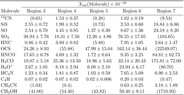
Ta-ble 10lists these calculated abundances, which are displayed in Figure6. Recall that
in the calculations of the hydrogen column density and mass presented in this section
we have adopted the dust temperature assumed by Leroy et al. (2015); Td= 35 K.
Some trends in our measured molecular abundances are apparent in Figure 6:
• For 13CN, SiS, SO, SO
2, HNCO, HC3N, and C4H, Region 5, the Region
asso-ciated with the central source, TH2, possesses the lowest abundance of the five Regions studied.
• For SiS, SO, HNCO, and HC3N, in addition to Region 5 possessing the lowest
abundance, Region 7, the region studied in this work which is the farthest from the NGC 253 nucleus, possesses the highest abundance.
• For those molecular species common to both studies, our derived molecular
abundances are within the same range of 5×10⁻⁹ to 5×10⁻¹⁰ as those derived
30 Mangum et al.
0h47m32.60s 32.80s
33.00s 33.20s
33.40s
RA (J2000) 22.0"
20.0" 18.0" 16.0" -25°17'14.0"
Dec (J2000)
1
2
3
4
5
6
7
8
9
Color: 365 GHz Continuum Contours: VLT
Br-NGC253
0.005 0.010 0.015 0.020 0.025
Continuum Flux (Jy/beam)
Figure 5. Comparison of the 365 GHz continuum (color) and VLT Brγ (contours; Rosen-berg et al. 2013) emission distributions toward the CMZ of NGC 253. Contour levels are
0.2, 0.4, 0.6, 1.0, 1.5, 2.0, 3.0, and 4.0 ×10⁻¹³erg cm−2s−1arcsec−2. The spatial resolution
for both images is shown in the lower-left corner. Red numbers indicate the locations of
the dense molecular transition regions identified byLeroy et al.(2015, Table 4). Note that
we have adopted the astronometry from Fern´andez-Ontiveros et al. (2009) to define the
absolute positions in the Brγ image.
These molecular abundance patterns could be related to the spatial distribution of energy sources, such as sources of cosmic rays and mechanical energy, within the NGC 253 CMZ. Past surveys designed to sample the dominant chemical processes in
NGC 253 (e.g.Mart´ın et al. 2006;Aladro et al. 2015) have noted the influence of the
burst of star formation on the energetics within NGC 253. To tease-out the relative dominance of different dense gas heating processes, models which predict the varia-tion in molecular abundances within starburst environments have been developed. In general, these models characterize the changes in molecular abundances as a function
of metallicity (z), volume density (n(H2)), radiation field intensity (G0), cosmic ray
rate (ζ), and mechanical heating (Γmech). These physical processes are then coupled
to chemical model networks to allow for the prediction of molecular abundances as a function of varying physical conditions. These molecular abundance predictions can then be used to guide our understanding of the abundance distributions measured in Galactic and extragalactic star formation regions. The adapted chemical-PDR
Table 10. NGC 253 Component Total Molecular Abundancesa
Xtot(Molecule)×10−10
Molecule Region 3 Region 4 Region 5 Region 6 Region 7
13CN (0.65) 1.53±0.37 (0.38) 1.02±0.19 (9.53)
SiS 2.55±0.72 1.99±0.52 (0.73) 2.53±0.60 18.84±6.86
SO 2.54±0.70 4.45±0.85 1.37±0.39 8.67±1.36 23.18±8.20
SO2 38.94±7.76 18.31±7.56 12.26±4.86 76.55±17.05 (104.65)
HNC 0.86±0.42 3.89±0.82 (5.88) 7.95±1.05 2.64±1.47
OCS 24.26±8.93 (55.88) 47.99±15.04 162.14±38.44 (22549.07)
HNCO 17.65±6.78 4.69±1.32 1.72±0.64 9.35±3.25 84.81±62.73
H2CO 10.87±5.18 25.36±13.50 18.96±5.63 32.14±20.43 175.81±72.00
H3O+ 2.67±1.05 8.18±2.94 6.08±2.10 23.94±6.17 (80.70)
HC3N 1.23±0.34 1.81±0.87 1.02±0.59 7.65±5.09 6.90±2.53
C4H 0.07±0.02 0.07±0.02 0.02±0.006 0.20±0.03 (0.47)
CH3CN (1.03) (0.4) . . . 0.63±0.25 3.18±1.89
CH3OH (41.00) (54.40) (43.82) 59.40±9.11 (1710.93)
aDerived from measured total optically-thin molecular abundances (Table 9) and
dust-continuum derived H2 column densities (Table 6). Upper limits, listed in parentheses,
are quoted as 3σ.
specifically designed to predict molecular abundances in extreme star formation envi-ronments such as starburst galaxies and very high star formation-rate ultra luminous infrared galaxies (U)LIRGs. Even though these two models have been used to pre-dict molecular abundances within somewhat different sets of physical conditions, in
general these models predict that when the cosmic ray ionization rate ζ is increased,
the abundances of molecular species other than simple ions such as OH+, CO+, CH+,
and H2O+ (none of which are part of this study) decrease. The range ofζ modeled in
these studies runs from the canonical Milky Way value of 2.6±0.8×10⁻¹⁷s−1(van der
Tak & van Dishoeck 2000) to 5×10⁻¹³s−1. This upper limit toζ is roughly ten-times
the cosmic ray ionization rate determined for NGC 253 from ultra-high energy cosmic
ray observations, which isζ '3.6×10⁻¹⁴s−1 (Acero et al. 2009), and is believed to be
consistent with cosmic ray densities in ULIRGs (Papadopoulos 2010). The supernova
rate which corresponds to the measured gamma-ray flux from NGC 253 is ∼0.1 yr−1
(Acero et al. 2009), which is most pronounced towards its nucleus7.
Given the existence of strong IR radiation fields in the NGC 253 CMZ, a note of caution is in order regarding the interpretation of rotational transition intensities for molecules which might be affected by radiative pumping of vibrational states
that subsequently experience radiative decay. HCN, HNC and HC3N (Section 8)
show vibrationally-excited emission in NGC 253. Rotational energy levels in other
0 20 40 60 80 100
Molecule
10
1210
1110
1010
910
810
7X(mol)
13CN SiS SO SO2 HNC OCS HNCO H2CO H3O+ HC3N C4H CH3CN CH3OH
NGC 253 Region Total Molecular Abundances
Region 3
Region 4 Region 5
Region 6 Region 7
Figure 6. Total molecular abundances, excluding13CO and C18O, derived from the total
molecular column densities listed in Table9. Limits are shown with downward arrows.
molecules, including H2CO (Mangum & Wootten 1993), can also be excited by
far-infrared emission, representing a potential unaccounted source of excitation of these molecules. Physical scenarios which attempt to describe infrared excitation of
molec-ular rotational energy levels in molecules (Carroll & Goldsmith 1981; Mangum &
Wootten 1993) tend to require that the sources of infrared emission be cospatial with
the molecular distribution. Our measurements of vibrationally-excited HNC and
HC3N emission (Section 8) suggest that this emission could possess similar spatial
distributions to their rotationally-excited counterparts. We would expect that if in-frared excitation through vibrational transitions was signficantly contributing to the purely rotationally-excited transitions that we measure, we would expect to see local maxima in their spatial distributions which correspond to peaks in the vibrationally-excited emission from a given molecule. We have found that Region 6 represents a
local maximum in vibrationally-excited HNC and HC3N emission (Section8),